HAL Id: hal-01857807
https://hal.archives-ouvertes.fr/hal-01857807
Submitted on 20 Dec 2019HAL is a multi-disciplinary open access archive for the deposit and dissemination of sci-entific research documents, whether they are pub-lished or not. The documents may come from teaching and research institutions in France or abroad, or from public or private research centers.
L’archive ouverte pluridisciplinaire HAL, est destinée au dépôt et à la diffusion de documents scientifiques de niveau recherche, publiés ou non, émanant des établissements d’enseignement et de recherche français ou étrangers, des laboratoires publics ou privés.
Molecular tagging velocimetry for confined rarefied gas
flows: Phosphorescence emission measurements at low
pressure
Dominique Fratantonio, Marcos Rojas-Cárdenas, Hacene Si Hadj Mohand,
Christine Barrot, Lucien Baldas, Stéphane Colin
To cite this version:
Dominique Fratantonio, Marcos Rojas-Cárdenas, Hacene Si Hadj Mohand, Christine Barrot, Lucien Baldas, et al.. Molecular tagging velocimetry for confined rarefied gas flows: Phosphorescence emission measurements at low pressure. Experimental Thermal and Fluid Science, Elsevier, 2018, 99, pp.510-524. �10.1016/j.expthermflusci.2018.08.001�. �hal-01857807�
Accepted Manuscript
Molecular Tagging Velocimetry for Confined Rarefied Gas Flows: Phosphor-escence Emission Measurements at Low Pressure
Dominique Fratantonio, Marcos Rojas-Cardenas, Hacene Si Hadj Mohand, Christine Barrot, Lucien Baldas, Stéphane Colin
PII: S0894-1777(18)30892-6
DOI: https://doi.org/10.1016/j.expthermflusci.2018.08.001
Reference: ETF 9567
To appear in: Experimental Thermal and Fluid Science
Received Date: 11 May 2018 Revised Date: 13 July 2018 Accepted Date: 2 August 2018
Please cite this article as: D. Fratantonio, M. Rojas-Cardenas, H. Si Hadj Mohand, C. Barrot, L. Baldas, S. Colin, Molecular Tagging Velocimetry for Confined Rarefied Gas Flows: Phosphorescence Emission Measurements at Low Pressure, Experimental Thermal and Fluid Science (2018), doi: https://doi.org/10.1016/j.expthermflusci. 2018.08.001
This is a PDF file of an unedited manuscript that has been accepted for publication. As a service to our customers we are providing this early version of the manuscript. The manuscript will undergo copyediting, typesetting, and review of the resulting proof before it is published in its final form. Please note that during the production process errors may be discovered which could affect the content, and all legal disclaimers that apply to the journal pertain.
1
Molecular Tagging Velocimetry for Confined Rarefied Gas Flows:
Phosphorescence Emission Measurements at Low Pressure
Dominique Fratantonio1, Marcos Rojas-Cardenas1, Hacene Si Hadj Mohand2, Christine Barrot1,
Lucien Baldas1, Stéphane Colin1*
1Institut Clément Ader (ICA), Université de Toulouse, CNRS, INSA, ISAE-SUPAERO, Mines-Albi, UPS, Toulouse, France
2Laboratoire des Fluides Complexes et Leurs Reservoirs-IPRA, UMR5150, CNRS/Total/Univ Pau Et Pays Adour, 64000, PAU, France
Keywords: microfluidics, gas flows, molecular tagging velocimetry, rarefied gas, phosphorescence
Abstract
Rarefied gas flows have a central role in microfluidic devices for many applications in various scientific fields. Local thermodynamic non-equilibrium at the wall-gas interface produces macroscopic effects, one of which is a velocity slip between the gas flow and the solid surface. Local experimental data able to shed light on this physical phenomenon are very limited in the literature. The molecular tagging velocimetry (MTV) could be a suitable technique for measuring velocity fields in gas micro flows. However, the implementation of this technique in the case of confined and rarefied gas flows is a difficult task: the reduced number of molecules in the system, which induces high diffusion, and the low concentration of the molecular tracer both drastically reduce the intensity and the duration of the exploitable signal for carrying out the velocity measures. This work demonstrates that the application of the 1D-MTV by direct phosphorescence to gas flows in the slip flow regime and in a rectangular long channel is, actually, possible. New experimental data on phosphorescence emission of acetone and diacetyl vapors at low pressures are presented. An analysis of the optimal excitation wavelength is carried out to maximize the intensity and the lifetime of the tracer emission. The experimental results demonstrate that a little concentration of about 5-10 % of acetone vapor excited at 310 nm or of diacetyl vapor excited at 410 nm in a helium mixture at pressures on the order of 1 kPa provides an intense and durable luminescent signal. In a 1-mm deep channel, a gas flow characterized by these thermodynamic conditions is in the slip flow regime. Moreover, numerical experiments based on DSMC simulations are carried out to demonstrate that an accurate measurement of the velocity profile in a laminar pressure-driven flow is possible for the rarefied conditions of interest.
2
1. INTRODUCTION
In the last two decades, micro-electro-mechanical systems (MEMS) have received a lot of attention due to their appealing properties of low volume and weight, and for their possible applications in a very wide variety of scientific fields. Specifically in the gas microfluidic sector, several interesting applications have recently been developed. It is the case of micronozzles for space applications [1], micro-actuators for aeronautical applications [2], micro heat exchangers [3], and Knudsen pumps [4], to name just a few. The growing interest towards these micro-devices has brought the scientific community to dedicate great research effort towards heat and mass transfer analysis in gas flows at microscale.
The size reduction in micro gas systems amplifies the thermodynamic disequilibrium of the flow as a consequence of the increased gas rarefaction. This phenomenon results from a decrease in the number of intermolecular collisions inside the control volume. The Knudsen number, ⁄ , where is the mean free path and is the characteristic size of the system, identifies the degree of gas rarefaction. Most of the microfluidic devices works in the slip flow regime, with in the range 10 ; 10 , which is to be considered as a slightly rarefied gas flow regime. This regime can be reached either in a microfluidic device, where is low, or in a bigger system at low pressure, which results in a high mean free path . In this rarefaction regime, the continuum representation of the flow is still acceptable for fluid particles that are far enough from the system’s solid boundaries, i.e. at a distance larger than the well-known Knudsen layer thickness which is considered to be on the order of . However, for those systems that involve wall-gas interactions, e.g., in micro channels or in channels at low average pressure, the number of collisions between the wall surfaces and the gas molecules gains importance with respect to intermolecular collisions, thus producing a thermodynamic non-equilibrium state of the gas in the vicinity of the wall. At a macroscopic level, this produces a velocity slip and a temperature jump at the wall [5], i.e., discontinuities of kinematic and thermodynamic parameters between fluid and surface. Therefore, even if the Navier-Stokes-Fourier equations still hold, specific boundary conditions must be introduced to take into account these discontinuities at the wall. Various forms of boundary conditions for both continuum medium and kinetic theory [6] derived models have been proposed in the literature. All of them depend on accommodation coefficients that vary as a function of the wall properties and gas species, andwhich determination is still a difficult task. Experimental data are required to evaluate these coefficients and to validate the proposed models.
3
Most of the experiments performed on rarefied gas flows in channels indirectly analyze the effects given by the velocity slip and temperature jump at the wall by measuring global quantities, such as mass flow rate, inlet and outlet pressures and temperatures [7-14]. To the best of our knowledge, there are no experimental data in the literature that provide local analysis of the rarefaction effect at the wall.
One of the most widely used techniques for local investigation of the velocity field in both liquid and gas flows is the particle image velocimetry (PIV). Its application to microfluidic systems is known as μPIV. Although this technique can provide accurate data related to liquid flows in micro-channels [15,16,17], the application of μPIV has been very limited up to now in gas micro flows [18,19]. The main problem is related to the tracer particle size. Beside the technological difficulties in generating particles with a diameter less than 1 μm, the particle size should be small enough to guarantee that the particles faithfully follow the fluid flow and big enough to reduce Brownian motion noise [20] that makes the cross-correlation operation inaccurate. For these reasons, μPIV has never been applied for velocity measurements in rarefied gas flows.
Our team has developed a molecular tagging velocimetry technique with the purpose of directly quantifying the slip velocity at the wall and measuring the overall velocity profile for a pressure-driven rarefied gas flow in a channel of rectangular section.
The molecular tagging velocimetry (MTV) is an optical technique with low intrusiveness. Differently from PIV where the tracer is made of particles, this alternative velocimetry technique is based on the exploitation of a molecular tracer able to emit light for a certain duration after having been excited by a UV-light source. Among all the possible versions of this technique, 1D-MTV by direct phosphorescence of acetone or diacetyl vapors has been chosen for the present work. The basic principle of this technique is depicted in Figure 1. The velocity profile is deduced from the streamwise displacement of the tracer molecules initially tagged by the laser along a line perpendicular to the gas flow direction.
4
Figure 1. Basic principle of 1D-MTV by direct phosphorescence, for a gas flowing in a plane channel from left to right.
1D-MTV by direct phosphorescence is the simplest and the most straightforward version of MTV, since it requires only one laser system, in contrast to other implementations, such as RELIEF [21] or PHANTOMM [22] techniques, which require more than one photon source or cannot be applied to gas flows. Laser sources with high repetition rates can be useful for velocimetry in unsteady flows. For application to steady gas flows, a frequency of the order of 10 Hz provided by common flashlamp-pumped lasers is high enough to accurately measure velocity fields.
1D-MTV by direct phosphorescence has already been applied to non-rarefied external supersonic or hypersonic turbulent gas flows [23, 24], to rarefied supersonic jets [25] and to non-rarefied gas flows in millimetric channels [26, 27]. However, some difficulties have prevented until now the successful application of this technique to confined rarefied gas flows. Since the laser beam can hardly be smaller than about 30 μm for technological reasons, the height of the channel is constrained to be not smaller than about 1 mm, in order to keep a reasonable spatial resolution. Consequently, Knudsen numbers corresponding to the targeted slip flow regime can only be reached by decreasing the average pressure of the gas-tracer mixture.
Our research team has already made progress in the direction of applying MTV in rarefied conditions. Samouda et al. [26] have demonstrated that the technique can provide good results in a millimetric rectangular channel for a non-rarefied gas flow at atmospheric pressure and ambient temperature. However, they noticed that a deduction of the velocity profile by assuming it was simply homothetic of the displacement profile resulted in an artificial velocity slip at the wall, which was totally unexpected for the employed Knudsen numbers. Subsequently, Frezzotti et al. [28] explained this unexpected phenomenon at the wall as a
5
consequence of a combined effect of advection and molecular diffusion of the tracer in the background gas flow. Moreover, the same authors proposed a numerical method based on a simple advection-diffusion equation that was able to correctly reconstruct the velocity profile from the displacement profile. By means of the Direct Simulation Monte Carlo (DSMC) method, it was possible to numerically verify the existence of a displacement slip at the wall caused by the advection-diffusion mechanism and not linked to a velocity slip at the wall. A reconstruction method of the velocity profile from the displacement profile was developed and validated with numerical experiments. Si Hadj Mohand et al. [27] successfully applied this reconstruction method on MTV data in a millimetric channel and correctly extracted the velocity profile at atmospheric and sub-atmospheric pressures down to a minimum average pressure of 50 kPa. At this pressure level in a 1-mm deep channel, the flow is still in a non-rarefied regime.
Lower pressures reduce, however, the tracer molecule concentration and increase the molecular diffusion. The combination of these two effects drastically decreases the phosphorescence signal intensity as well as its lifetime. Therefore, it is necessary to experimentally explore the phosphorescence emission of different molecular tracers and look for a physical condition that makes the application of the 1D-MTV to the rarefied case feasible.
For that purpose, the present work is intended to show new results in terms of acetone and diacetyl phosphorescence as a function of total pressure, molecular tracer concentration, excitation wavelength, and gas species, in low pressure conditions. These experimental data reveal which Knudsen numbers can be achieved in a pressure-driven flow while still having a durable and visible phosphorescence signal from the tracer. In this work, the Knudsen number:
/ , (1)
is defined as the ratio of the average mean-free path of the gas mixture, composed of the background gas and the tracer gas molecules, to the height of the channel. In the light of these new experimental results, a numerical analysis of the tracer advection-diffusion inside the gas mixture and numerical experiments by means of DSMC are carried out to demonstrate that, for the considered rarefied conditions, the molecular tracer displacement is measurable by means of the MTV setup presented in this work and that the velocity profile can be correctly reconstructed.
6
2. EXPERIMENTAL SETUP
2.1 MTV setup
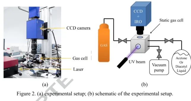
The present work aims to analyze the intensity and the lifetime of the phosphorescence emission of the molecular tracers in different thermodynamic conditions. For this reason, the light emission is analyzed with a gas-vapor mixture at rest in a small chamber. Figure 2a shows the experimental setup, which is composed of three main parts: the gas circuit, the laser, and the recording image system. Figure 2b represents a schematic view of the same experimental setup.
(a) (b)
Figure 2. (a) experimental setup; (b) schematic of the experimental setup.
The absorption spectra of acetone and diacetyl are, respectively, in the range 240-340 nm and 250-470 nm [29, 30]. An OPOlette HE355LD laser has been used for all the experiments, since it allows to provide the proper UV excitation for both acetone and diacetyl. The OPOlette HE355LD is a tuneable laser that can provide a pulsed laser at a wavelength in the 210-355 nm and 410-710 nm ranges. In order to generate these ranges of frequency, the nonlinear crystals are pumped at 355 nm by means of a Nd:YAG pumping laser, which generates laser pulses at 1064 nm, coupled with a Third Harmonic Generator (THG). The OPOlette HE355LD allows to adjust the delay between the Q-switch trigger signal and the flashlamp trigger signal for controlling the output energy. The maximum laser energy moves from about 0.9 to 0.2 mJ in the range [250, 340] nm and between 5 and 8 mJ in the range [410, 470] nm. The laser pulses last 7 ns each and are shot at a rate of 20 Hz. The beam diameter at the exit of the laser box is of 4 mm, and it is focused by means of a diaphragm valve and of a system of lenses down to about 310 μm in the region captured by the camera. The diameter of the laser beam is estimated
7
by taking the full width at half maximum (FWHM) of the Gaussian emission distribution recorded 5 ns after the laser excitation.
The energy density of the laser beam is limited to avoid damaging the laser access window. Thus the average laser energy is set between 30 and 60 μJ. Nevertheless, the lowest energy density for locally damage the window is actually at least one order of magnitude higher than the one employed in this work. For the current study it has been decided to work with a large laser beam diameter for a more accurate investigation of the diffusion process of the gas tracer within the background gas. However, the energy density per unit area is in the same order of magnitude as the energy densities that can be used for MTV analysis in a sub-millimetric confined flow.
Therefore, even though the diaphragm valve allows to further decrease the diameter of the beam down to about 30 μm for velocimetry purpose, a larger beam is used at this stage of the project to exploit at best the spatial resolution of the charge coupled device (CCD) and to analyze more easily the gas diffusion mechanisms.
The static gas cell is equipped with two optical accesses: an optical window in Suprasil® for the laser beam access, and an optical window in Borofloat® on the top of the cell that is transparent to the light emitted by the tracer. Three gas lines are connected to the static cell: one for channeling acetone or diacetyl vapor, one for channeling the background gas, and one for vacuuming the cell. These three gas-vapor lines are regulated by Swagelok® valves. The acetone or diacetyl vapor is generated from a bottle containing the fluid in its liquid form. The bottle is directly connected to the cell and its vertical position ensures that only vapor is pumped out. The cell is vacuumed during 2 days in order to have a complete outgassing of the unwanted molecules adsorbed by the inner walls. This procedure is repeated every time before using a new type of vapor or gas inside the cell. Working with a static gas cell rather than a flowing gas cell [31] makes the experimental setup much simpler, permits an easier and better control of pressure and temperature conditions of the mixture, and reduces the waste of carrier gas and tracer vapor, since the same mixture can be employed for more than one acquisition. Moreover, the relative concentrations of gas and vapor can be accurately controlled, since the mixing is directly done inside the cell by simply adding the right amount of partial pressure. The use of a static cell, however, requires attention on some issues, such as gas mixing time, material compatibility with acetone and diacetyl, inner wall adsorption of acetone and diacetyl, and the occurrence of molecular photolysis. The mixing process is relatively fast, considering the small volume of the cell. Moreover, for checking the absence of significant photolysis, it has been verified that, for the laser intensities used, the signal intensity did not vary in time during a
8
series of many successive laser shots. The main issue is the adsorption of the tracer molecules on the inner walls, which causes a monotonic drop of the nominal pressure in the cell. However, a stable pressure condition is easily attained by refilling the cell with acetone or diacetyl in order to saturate the adsorption phenomenon and reach a stationary state.
A 12-bit Imager Intense (LaVision®) progressive scan CCD coupled with a 25-mm intensified relay optics (IRO) has been employed for the image recording. The optical system for collecting the emitted light is made of 105 mm f: 2.8 and inverted 28 mm f: 2.8 Micro Nikkor lenses. The resolution of the CCD is 1376 (horizontal) × 1040 (vertical) pixels. Since the phosphorescence emission has very low intensity, a binning process is required for increasing the sensitivity to light of the CCD at the expense of reducing the spatial resolution. If not otherwise specified, a 4 × 4 binning is operated for all the experimental data presented in this work; the resolution of the CCD is, thus, reduced to 344 x 260 pixels. The overall magnification given by the external optical system and the internal optical collector of the IRO and CCD is about 1.7. As the CCD covers an actual area of 8.87 mm × 6.71 mm, the field of view is 5.29 mm × 4 mm. Consequently, each pixel corresponds to an area of 3.8 μm × 3.8 μm without binning and to 15.2 μm × 15.2 μm with a 4 × 4 binning. The digital conversion of the number of photons collected on one pixel of the CCD sensor provides a certain number of “counts”. The IRO is made of a S20 type photocathode and a P46 phosphor plate. The laser trigger, the camera shutter, and the IRO trigger are all synchronized by a programmable timing unit (PTU) with a precision of 5 ns. The main parameters that can be controlled for each record are the delay time between the IRO trigger and the laser trigger, the IRO gate ∆ , i.e., the time interval of light integration, the IRO amplification gain G and the exposition time of the CCD detector.
2.2 The on-chip integration technique
Since this study involves low tracer concentrations and requires limited laser energy levels to preserve the integrity of the access window, the amount of light that one single laser excitation can provide is very low. As a matter of fact, recording on the CCD the phosphorescence emission given by one pulse laser excitation results in a more or less blank image. For this reason, the on-chip integration is used. This technique allows to collect in one single image the light generated by more than one laser excitation. By keeping the CCD camera shutter open, the IRO is activated at the same delay time t and during the same gate Δ after each laser excitation. Since the phosphorescence emission is weak, the IRO amplification is always
9
exploited at its maximum, so that its gain is fixed to 100 %. The final image is given by the average of images that are each the result of the integration of laser pulses. A higher number of averaged images can increase the quality of the resulting image by reducing the data fluctuations. It cannot, however, increase the light intensity. Statistical fluctuations are produced during all phases of the acquisition process, namely the excitation, the photon emission, and the acquisition phase. The laser energy and its spatial distribution fluctuate, as well as the absorption rate and the spatial distribution of the molecular tracer. The photo-luminescence emission is affected by a Poisson statistical noise, also called “photonic noise”, which gives an uncertainty that behaves as the square root of the number of emitted photons [32]. It constitutes the dominant source of image noise at high intensifier gain and it cannot be avoided even under ideal imaging conditions where all sensor-based sources of noise are removed. Moreover, although the photonic noise increases with signal intensity, this noise component is relatively weaker at higher signal levels. In the acquisition process, the photo cathode of the IRO is affected by the same Poisson statistical noise during the generation of electrons, and other noise sources are generated in the amplifier and by the CCD cells themselves. From the point of view of MTV application, there is not much interest in evaluating the statistical uncertainties on the emitted light intensity. In fact, the velocimetry technique requires precision in evaluating the molecular displacement and the time separation between two images. The spatial precision is mainly determined by the signal to noise ratio (SN) of the image and by the CCD resolution of the camera. For the lowest pressures employed in this work the SN becomes the most important source of uncertainty. In order to improve the SN, one should consider integrating a higher number of laser pulses and increasing the number of averaged images. The temporal precision is defined by the synchronization capability of the PTU, which is about 5 ns. However, the main concern of this experimental analysis is to assure the existence of a visible and exploitable signal even at low pressures, without paying too much of attention to the accuracy of the emitted light intensity. A higher number of laser pulses increases the recorded light intensity and reduces the statistical fluctuations. Figure 3a shows the light intensity amplification due to an increasing number of laser pulses, from 10 to 2000. The data refer to the phosphorescence emission of acetone vapor at a pressure p = 3 kPa, excited by a laser beam at 266 nm. The relationship is not exactly linear: as the number of laser pulses integrated in one image grows, the light amplification tends to decrease. The main limitation in increasing the number of laser pulses or averaged images is given by the recording time, which linearly increases with these two parameters. Since our experiments deal with a weak source of light, a high number of laser pulses and a limited number of averaged images is
10
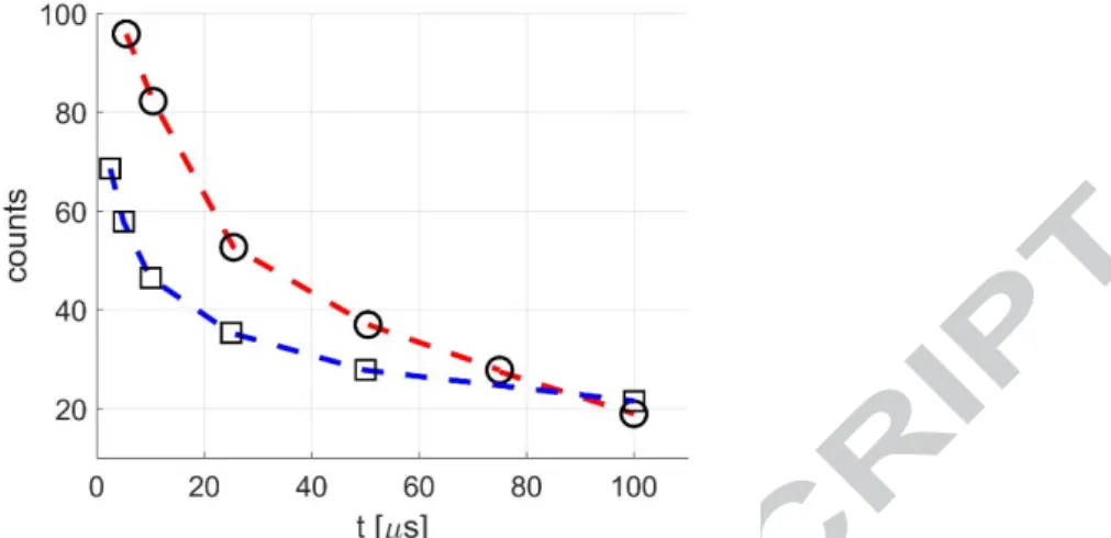
preferred. Alternatively, the IRO gate can be increased. In this way, the acquisition time does not change. In the view of the application of the MTV to gas flows, the IRO gate should be, however, kept lower than the characteristic time of the flow in order to be able to accurately evaluate the molecular displacement. The relationship between the amount of light recorded and the duration of the IRO gate is linear, as proved by the data of Figure 3b. Even though the emission intensity decreases in time, the linearity of the recorded signal with respect to the IRO gate still holds since the signal intensity at 50 µs and 100 µs after the laser excitation varies only of 0.1% during 2 µs of the IRO gate opening.
(a) (b)
Figure 3. (a) Emission intensity of acetone vapor at 3 kPa and 293 K as a function of the number of laser pulses integrated in one image. The data refer to the phosphorescence emission at t = 50 μs after the excitation, and result from the average
of = 10 images; (b) phosphorescence emission of acetone vapor at 5 kPa and 293 K as a function of the IRO gate. Data shown are for t = 50 μs, = 100 (O); t
= 100 μs, = 100 (▽); t = 50 μs, = 50 (+); t = 100 μs, = 50 (✱).
Another recording feature that can be modified to control the signal intensity is the binning operation. All the experimental data presented in this work have been acquired by employing a 4 × 4 binning, i.e., a matrix of 4 × 4 pixels is grouped to form a bigger pixel. Even though the spatial resolution of the image is decreased by 4 in each direction, this operation should provide a signal 16 times more intense with respect to an acquisition without binning. This aspect has been verified. Figures 4a and 4b show the emitted light with the same acquisition parameter without and with binning, respectively. By applying the above described fitting procedure to compute the signal intensity, the ratio of the signal intensity with binning over the signal
11
intensity without binning is of about 15, which is close to the expected value. By keeping this in mind, even though all the experimental data here presented refer to acquisitions made with a 4 × 4 binning, it is ascertained that an image with higher resolution and 16 times less bright can be obtained.
(a) (b)
Figure 4. Raw images of diacetyl phosphorescence emission at = 5 kPa, 293 K, and for t = 2 μs after the excitation. The images represent the collection of 100 laser
pulses, (a) without binning and (b) with 4 4 binning.
2.3 Image processing procedure
In the experimental analysis, the raw image is averaged along the direction of the laser beam and, then, a Gaussian fitting is carried out, as shown in Figure 5.
(a) (b)
Figure 5. Example of raw image and image processing procedure; (a) phosphorescence emission of pure acetone 10 μs after the laser excitation at 5 kPa for 100, 10, Δ 100 ns, and 100%; (b) Gaussian fitting (red line) of the emission profile (blue circles) that results from the averaging along the y-direction of the raw image shown in (a).
12
The employed fitting function has the following expression: ,
2 , (2)
where , , , and are the fitting coefficients. The degree of freedom, , is introduced to take into account the background emission, which is never zero. The CCD cells produce themselves an inhomogeneous strong dark-noise, which is linked to the thermal energy distribution of the electrons in the silicon [33]. This type of noise is greatly reduced by cooling down the CCD camera to about -10 °C, but relatively long camera exposition heats the CCD cells to a level such that the dark-noise pattern is clearly visible on the acquired image. However, for each acquisition, the dark-noise image is recorded without laser excitation and then subtracted from the final image. The background offset is, therefore, not due to this noise component and only the light reaching the CCD cells contributes to the result. The background light offset can be due to reflected UV light and/or to phosphorescence emissions by out-of-the-beam molecules, excited either by diffused or reflected UV photons. Even those tracer molecules that have been adsorbed by the wall can be excited in this way. Diacetyl vapor is particularly sensitive to the adsorption phenomenon, and the background emission is more intense than in the case of acetone vapor. Parameter represents the amplitude of the Gaussian signal. More precisely, its time evolution is strictly linked to the phosphorescence lifetime of the excited tracer. Since this parameter is not affected by the diffusion mechanisms, the analysis of can provide important information about the photoluminescence process. Coefficient corresponds to the variance of the Gaussian and its evolution in time gives information about the diffusion rate of the excited tracer molecules inside the background gas mixture. Finally, coefficient represents the position of the Gaussian peak. Due to possible small perturbations in the position of the laser beam and to fluctuations in the laser energy pattern, this value can be slightly different from one acquisition to the other. While this last parameter is not of much interest for the experimental analysis presently described, the MTV technique is based on the accurate measurement of .
The averaging operation of the collected light along the laser beam direction reduces the statistical fluctuations of the emission distribution. The same result could have been achieved by simply averaging more images, but at the expense of a higher amount of time for the acquisition. As for the application of the MTV, the operation of averaging along the laser beam cannot be applied, since the tagging line deforms as the excited tracer molecules follow the gas
13
flow direction. An independent Gaussian fitting must be applied on each row of pixels for detecting the Gaussian peak position and thus tracking the molecular displacement along the tagging line. In this scenario, the reduction of the statistical fluctuations necessarily requires averaging more images.
The fact that the signal can be approximated by a Gaussian is not as straightforward as it seems. The shape of the laser energy distribution that excites the molecular tracer is more complex than a simple Gaussian. Even if the light beam at the exit of the laser has a Gaussian intensity pattern, this distribution is modified by a circular obturator positioned before the focalization lenses. Therefore, the final energy distribution of the light beam takes the form of a circularly-truncated Gaussian. Thus, the acquired signal cannot be precisely described by a Gaussian profile. However, the molecular diffusion smooths the distribution of excited molecules towards a Gaussian distribution quite quickly after the excitation time. Furthermore, if the IRO gate, i.e., the integration time, is small enough with respect to the luminescence and diffusion rates, the Gaussian fitting can be considered as a good approximation of the signal.
The Gaussian peak value is then taken as the main characterization of the signal intensity at a given instant t after the laser excitation and for the thermodynamic conditions under consideration.From Eq. (2), the Gaussian peak corresponds to the following expression:
,
2 . (3)
As it can be seen from Eq. (3), the Gaussian peak value is determined by , , and , which can be affected both by phosphorescence lifetime and/or diffusion. The Gaussian peak is an interesting quantity for characterizing the time evolution of the signal, as it contains information related to both phenomena. Moreover, in MTV the Gaussian peak is used for tracking the displacement of the tagged line and, thus, is a fundamental quantity for carrying out velocity measurements. Low SN values can greatly affect a precise measurement of the position of the Gaussian peak. For the lowest pressure employed in this work, that is for low SN, and for an acquired image obtained with Nl = 500, Ni = 10, and a 4 × 4 binning, the peak
position of the Gaussian fitting applied on each row of pixels of the image fluctuates along the laser beam direction with a standard deviation that can vary from 2 to 10 pixels, depending on the acquisition delay time and the IRO gate.
2.4 Molecular tracer properties
After UV-laser excitation, acetone vapor emits a certain amount of light, which can be described as the sum of two components: a strong light emission that lasts for only some
14
nanoseconds, which is commonly defined as fluorescence, and a less intense light emission that can last even for hundreds of microseconds or about a millisecond, which is known as phosphorescence. The definitions of fluorescence and phosphorescence emissions are not based on the intensity and the duration of the emission but on the type of intramolecular electronic transition that makes an excited molecule come back to its ground electronic state [34]. Similarly, diacetyl is characterized by both fluorescence and phosphorescence emissions. However, the photoluminescence characteristics of diacetyl are quite different from those of acetone. Its phosphorescence emission is much more intense than the fluorescence emission and has a higher lifetime than the acetone phosphorescence. This difference in duration and intensity is due to the fact that the phosphorescence quantum yield, namely the percentage of excited molecules that re-emit “phosphorescent” photons, is about 1.8% and 15%, for acetone and diacetyl respectively [29]. For both molecular tracers, only the phosphorescence component of the emission is exploited, since the lifetime of the fluorescence is too short for detecting a macroscopic gas displacement in microfluidic applications of interest.
While acetone has a saturated pressure vapor of 24 kPa at 20 °C and has relatively low toxicity, diacetyl has a lower saturated pressure vapor, about 6 kPa at 20 °C, and its toxicity is quite higher, such that some precautions must be taken during its handling. Although the highest diacetyl pressure that can be employed at ambient temperature is relatively low, this is not a limitation for the current work, as the targeted rarefied regime requires even lower pressures.
The acetone luminescence has already been implemented in imagery techniques for measuring temperature, pressure, concentration, and velocity fields [25, 29, 31, 35, 36]. Even if the use of diacetyl as a potential molecular tracer in gas flows has been already analyzed in the past, only a few results can be found in the literature [37]. In the chemistry’s literature, the photoluminescence of acetone and diacetyl vapor has been extensively analyzed [38, 39], as it is a tool for studying the internal electronic structure of these molecules, which are the simplest and most representative molecules of the ketone compounds. However, the available experimental data relative to the dependency of phosphorescence lifetime and intensity on the partial pressure of acetone or diacetyl are not enough for understanding if these molecular tracers can be employed for successfully applying the MTV technique to the case of rarefied and confined gas flows.
15
3. EXPERIMENTAL RESULTS
3.1 Optimization of phosphorescence intensity with excitation wavelength
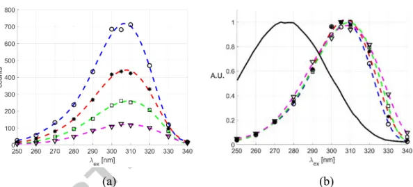
For a channel of 1 mm in height and for a helium-acetone mixture with a molar fraction 5% of acetone vapor, an average total pressure of about 1400 Pa is required to get a gas flow at 0.01. For these thermodynamic conditions, the phosphorescence signal provided by the acetone molecules when excited by a 266 nm laser beam has been proven to be insufficiently intense and durable in time, preventing from a successful application of MTV. However, we have observed that a different excitation wavelength can provide higher phosphorescence emissions. Even if the absorption spectrum of acetone has a peak at 271 nm and goes rapidly down at 340 nm, the strongest emission is obtained for an excitation wavelength between 300 and 310 nm. Figures 6 and 7 show this result, demonstrating that the phosphorescence intensity can be more than 12 times its value obtained at 260 nm. In Figures 6a and 7a, data represent the phosphorescence emission of pure acetone vapor at = 15 kPa and = 1.5 kPa, respectively. For all excitation wavelengths, the pulse energy was set to 30 µJ and the laser beam diameter was kept to about 310 µm. The energy density is thus estimated to be 0.04 J/cm2. The different curves refer to different delay times after laser excitation. For a better analysis of the amplification factor that can be obtained by modifying the excitation wavelength, phosphorescence data are normalized with respect to the highest value of the light intensity emission. In Figure 6b, the emission provided by acetone vapor at 15 kPa is maximum for excitation wavelengths between 305 and 310 nm, regardless of the considered delay time. At 1.5 kPa (Figure 7b), no visible signal for excitation wavelengths equal or lower than 270 nm could be recorded. Figure 7b demonstrates that even at low pressure the highest amplification is given for excitation wavelengths between 305 and 310 nm. This non-intuitive experimental result can be explained by the fact that even if for these wavelengths, acetone vapor absorbs much less photons, the quantum yield of phosphorescence, namely the percentage of excited acetone molecules that effectively produce phosphorescence, is higher. This behavior results in a higher number of photons re-emitted by the acetone molecules and received by the CCD of the camera. Even if this phenomenon can be summarily explained by means of an overall quantum yield coefficient that describes the molecule’s journey from the excitation to the phosphorescence emission, the intramolecular transition processes that are involved in the light emission observed for an excitation at 310 nm are more complex than a simple excitation and de-excitation process. During the ’40s and ’50s, several chemistry oriented publications discussed about a “green” phosphorescence emitted by acetone molecules for an excitation
16
wavelength of 313 nm almost identical to the emission bands of the diacetyl’s spectrum [40]. Furthermore, Almy and Anderson [39] stated that they observed chemical evidences of diacetyl’s presence in acetone. Several authors hypothesized that the observed “green” phosphorescence, which increases the overall intensity of the signal recorded in the present work, is directly emitted by diacetyl molecules that form after a decomposition of acetone molecules and a subsequent recombination of two free acetyl radicals [41, 42]. However, diacetyl molecules do not emit when excited at 310 nm, a fact that was verified in the present work. In fact, the diacetyl’s excitation to the triplet electronic state that foreruns the phosphorescence emission is caused by molecular collisions with excited acetone molecules, following a molecular energy-transfer process known as photosensitization [43].
(a) (b)
Figure 6. (a) Phosphorescence emission of acetone vapor at 15 kPa and 293 K as a function of the excitation wavelength and for = 5 µs (O- -), 10 µs (✱- -), 20 µs (☐ - -), and 50 µs (▽- -) after the laser excitation. In (b) the same data as in (a) are normalized with respect to the highest light intensity recorded for each delay time.
The average laser intensity is 0.04 J/cm2, and the recording parameters are: 100, 10, 100%, and Δ 100 ns. The black solid line is the absorption
17
(a) (b)
Figure 7. (a) Phosphorescence emission of acetone vapor at 1.5 kPa and 293 K as a function of the excitation wavelength and for = 1 µs (O- -), 5 µs (✱- -), 10 µs (☐ - -), 25 µs (▽- -), and 50 µs ( - -) after the laser excitation. In (b) the same
data as in (a) are normalized with respect to the highest light intensity recorded for each delay time. The average laser intensity is 0.04 J/cm2, and the recording parameters are: 100, 10, 100%, and Δ 100 ns. The black solid
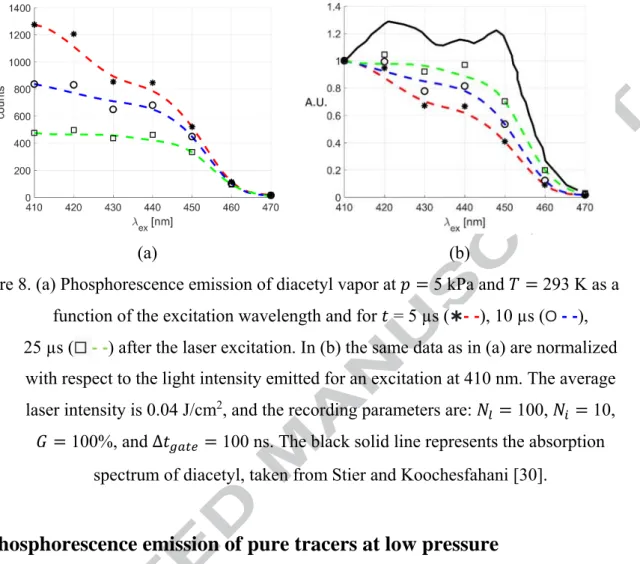
line is the absorption spectrum of acetone, taken from Lozano et al. [29]. Similarly, we investigated the phosphorescence emission of pure diacetyl vapor at 5 kPa for excitation wavelengths ranging from 410 to 470 nm. The results are shown in Figure 8. As for the data in Figure 6, the pulse energy was set to 30 µJ and the energy density was about 0.04 J/cm2 for all tested wavelengths. In this range, the emission has a maximum at 410 nm. It can be ascertained that the phosphorescence intensity does not follow the absorption spectrum when the excitation wavelength is changed. By moving from 410 to 470 nm, the signal tends to decrease, even if higher absorption can be found from 420 up to 450 nm. It is possible that a lower wavelength excitation could provide higher emission. Unfortunately, the OPOlette laser cannot provide excitation wavelengths between 355 nm and 410 nm, and, therefore, we could not investigate this part of the spectrum. In Figure 8b, the light intensity is normalized with respect to that provided by an excitation at 410 nm. Further investigations on the dependency of diacetyl phosphorescence from the excitation wavelength were carried out also at lower pressures. These experimental results are not here presented, since they only confirm, once again, that the excitation wavelength for which the signal intensity is maximized is 410 nm, at least in the range 410 to 470 nm.
18
(a) (b)
Figure 8. (a) Phosphorescence emission of diacetyl vapor at 5 kPa and 293 K as a function of the excitation wavelength and for = 5 µs (✱- -), 10 µs (O- -), 25 µs (☐ - -) after the laser excitation. In (b) the same data as in (a) are normalized with respect to the light intensity emitted for an excitation at 410 nm. The average laser intensity is 0.04 J/cm2, and the recording parameters are: 100, 10, 100%, and Δ 100 ns. The black solid line represents the absorption
spectrum of diacetyl, taken from Stier and Koochesfahani [30].
3.2 Phosphorescence emission of pure tracers at low pressure
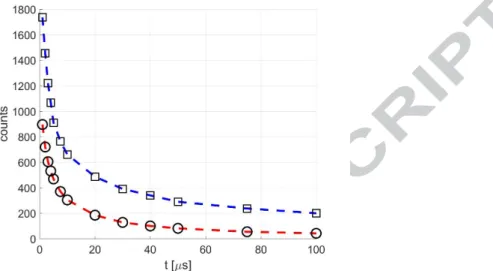
In the light of the results shown in Section 3.1, the wavelengths 310 and 410 nm have been chosen as optimum values for exciting the acetone and the diacetyl vapors, respectively. A direct comparison between the phosphorescence intensity given by acetone excited at 310 nm and that of diacetyl excited at 410 nm is shown in Figure 9. It represents the phosphorescence intensity of both tracers with respect to the delay time, from 1 to 100 μs, at p = 5 kPa. Each point in the figure corresponds to an average of 10 images, each image resulting from the integration of 100 excitations. The IRO gain and gate were 100 % and 100 ns, respectively. The decreasing of the signal is not just a result of the decay of the phosphorescence rate, which can be considered as proportional to the concentration of excited molecules as first approximation [39], but it also involves the diffusion mechanisms, since the figure represents the time evolution of the Gaussian peak of the signal, as previously explained in Section 2.3. The molecular diffusion spreads the excited molecules over the free space, so that the light collected in one pixel is drastically decreased. Figure 9 shows that the diacetyl signal can be from 2 to 5 times higher than the acetone signal, between 1 and 100 μs after the laser excitation. As previously discussed, since the growth of acetone emission intensity resulting from moving the
19
excitation wavelength from 266 to 310 nm is probably due to diacetyl’s emission, it was expected that from a direct excitation of diacetyl vapor a stronger signal intensity could be obtained.
Figure 9. Absolute intensity of phosphorescence emission in time for acetone (O- -) and diacetyl (☐ - -) at 5 kPa and 293 K, respectively excited at 310 and 410 nm. For all
data shown in the figure, the average laser intensity is 0.08 J/cm2, and the recording parameters are: 100, 10, 100%, and Δ 100 ns.
3.3 Phosphorescence emission of acetone and diacetyl in helium mixture at
low pressure
The phosphorescence lifetime of acetone excited at 310 nm and diacetyl excited at 410 nm have been analyzed in helium mixtures at low pressures and relatively low tracer concentrations. Figure 10 shows the time evolution of phosphorescence emission for acetone and diacetyl in helium at 1 kPa and with a tracer molar fraction 5% and 2% for the case of acetone and diacetyl, respectively. At this low acetone partial pressure level of 50 Pa, it is necessary to further increase the number of laser excitations integrated in each image for the highest delays in order to collect enough light. The data on acetone phosphorescence in Figure 10 have been recorded for 500, 10, 100%, and Δ 500 ns and shows an exploitable signal that lasts at least 100 μs. In a 1-mm deep channel, these conditions correspond to 0.015, which is within the slip flow regime.
20
Figure 10. Time evolution of phosphorescence emission in helium for acetone (O - -) and diacetyl (☐ - -) at 1 kPa and 293 K. For the data on acetone emission:
310 nm, 5%, 500, 10, 100%, and Δ 500 ns. For the data on diacetyl emission: 410 nm, 2%, 100, 10, 100%,
and Δ 500 ns. For all these data, the average laser intensity is 0.08 J/cm2. By mixing helium with diacetyl, a signal intensity comparable to that of acetone can be obtained, even for lower molecular tracer concentration and number of excitations per image. The data on diacetyl phosphorescence in Figure 10 have been recorded for 100, 10, 100%, and Δ 500 ns. In a 1-mm deep channel, these thermodynamic conditions provide a Knudsen number 0.016. A comparison of the data of Figure 10 shows that the two mixtures generate about the same absolute signal intensity. For instance, both tracers provide an intensity around 20 counts at 100 μs. However, a diacetyl-helium mixture with a concentration of 5% and 500 excitations per image would result in a signal almost 10 times higher than that provided by the acetone-helium mixture.
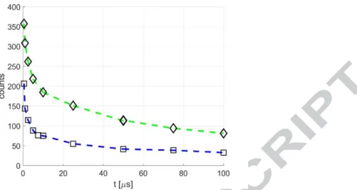
By increasing the diacetyl molar fraction, a strong signal can be obtained even at lower pressures. Figure 11 shows the phosphorescence emission in time for a diacetyl-helium mixture with a total pressure of 500 Pa and with 10 % and 20 % of diacetyl molar concentration. In a 1 mm deep channel, these thermodynamic conditions correspond to 0.027 and 0.022, respectively. The acquisition parameters are the same as those used for the data of Figure 10.
21
Figure 11. Time evolution of diacetyl phosphorescence in helium at = 500 Pa and 293 K for diacetyl molar fractions 10% (☐ - -) and 20% (◇ - -). The recording
parameters are 100, 10, 100%, and Δ 500 ns. For all data shown in the figure, the average laser intensity is 0.08 J/cm2, and the excitation wavelength is 410 nm. However, by comparing the data of Figures 10 and 11, it can be noticed that the signal intensity is far higher in Figure 11, even if the mixture has lower pressure. This is because the data of Figure 10 refer to a diacetyl-helium mixture at 1 kPa with only 2 % of diacetyl, that is a diacetyl partial pressure of 20 Pa. In Figure 11, although the gas mixture has a total pressure two times lower, diacetyl partial pressure is 50 Pa and 100 Pa for molar fractions of 10 % and 20 %, respectively. Figure 12 shows the raw images acquired for the mixture at 10% for = 10, 25, and 50 μs. It is worthy to remind that these images have been taken with the minimum effort in terms of laser pulses and averaged images number. Clearly, higher quality images can be obtained by increasing and , which are here set to 100 and 10, respectively.
22
(a) (b)
(c)
Figure 12. Raw images of diacetyl phosphorescence emission in helium at = 500 Pa and 293 K for a diacetyl molar fraction 10% at (a) t = 10 μs, (b) t = 25 μs, and
(c) t = 50 μs. The images refer to the data from Figure 11 at 10%.
4. FEASABILITY OF MTV APPLICATION TO RAREFIED
GAS FLOWS IN SLIP REGIME
The analysis presented above demonstrates that both acetone and diacetyl gas tracers can provide a durable and intense phosphorescence signal in slip flow regime conditions. It has been observed, in particular, that, in a gas mixture of helium at 1 kPa with a tracer concentration of about 5%, the phosphorescence emission lasts even for 100 μs after the laser excitation. For a channel with a height 1 mm, this thermodynamic condition corresponds to a Knudsen number 0.015, whether acetone or diacetyl is used. It has also been shown that by further reducing the pressure to 500 Pa and by increasing the tracer concentration to 10 %, a strong signal can be obtained up to 0.025.Knudsen numbers in the range [0.015; 0.025], which
23
are within the slip flow regime, correspond, therefore, to rarefaction conditions that can be experimentally investigated by means of MTV.
However, the fact that an exploitable phosphorescence signal is still present in these thermodynamic conditions cannot demonstrate by itself the feasibility of the application of the MTV technique to internal gas flows in the slip regime. The data presented in Section 3 on the phosphorescence lifetime of acetone and diacetyl have been carried out for a quiescent gas mixture in a non-confined environment. These data take into account the weakening effect of the signal due to the diffusion of the tracer molecules inside the background gas, but they do not take into account the conjugated effects of advection and diffusion on the molecular tracer in a confined environment.
The diffusion process combined with the velocity gradient perpendicular to the wall deforms the tagged line in such a way that a derivation of the velocity profile from the simple measurement of the streamwise tracer displacement does not provide correct results. As a matter of fact, Frezzotti et al. [28] demonstrated that a specific reconstruction method is needed to correctly extract the velocity profile from the measurement of the displacement profile of the tagged gas molecules, which are subjected to Taylor dispersion. Even for non-rarefied gas conditions, in which no slip velocity is expected at all, a displacement slip at the wall is measured by the MTV technique. This displacement slip has already been experimentally observed by Samouda et al. [26] and analyzed by Si Hadj Mohand et al. [27] for gas flows at atmospheric and sub-atmospheric pressures, respectively. At lower pressures, the advection-diffusion process can distort the displacement profile to such an extent that even the reconstruction method could not be sufficient to accurately measure the gas-mixture velocity profile. For the limit case scenario of high Knudsen numbers, the displacement profile of excited molecules tends asymptotically to an almost flat profile, from which the velocity information cannot be retrieved [28]. Even though the magnitude of the displacement is definitely large and measurable by means of the MTV technique, the reconstruction method may fail to provide the correct velocity profile in the case where the shape of the displacement profile is hidden by the CCD resolution and/or experimental inaccuracies. It is, therefore, necessary to carefully verify our ability to accurately measure the displacement profile that should form in specific rarefied conditions where a durable and intense phosphorescence emission is still present.
In this perspective, numerical experiments of the molecular advection and diffusion of the gas mixture are carried out by DSMC. These numerical results allow (i) to predict the shape of the
24
displacement profile in the thermodynamic conditions of interest and (ii) to verify if an accurate reconstruction of the velocity profile of the gas flow is possible.
4.1 Generation of numerical experiments by DSMC simulations
DSMC simulations of the gas-tracer mixture flow in a channel with a height 1 mm are carried out for Knudsen numbers in the range [0.015; 0.025] for the case of a plane laminar pressure-driven flow. The domain of the mathematical problem is defined by two parallel infinite plates perpendicular to the y-direction. The gas flows in between the two plates along the x-direction. The computational domain has open boundaries in the streamwise x- and spanwise z-directions. Since the 2D steady pressure-driven flow is invariant along these two directions, the computational cells are distributed only along the y-direction, which corresponds to the direction of the height of the channel. The axis of the channel is positioned at 0. For all considered cases, 500 cells along the height of the channel and 1 million test particles are employed. The steady pressure-driven flow is obtained as a result of the equilibrium between the viscous stresses and a uniform force applied to all particles in the computational domain. The force has been adjusted so that the maximum value of velocity of the attained steady state velocity profile is 30 m/s for all numerical experiments here shown. The corresponding Mach number is 0.039, so that the compressibility effects could be considered as negligible. Once the steady velocity profile is attained, the tracer molecules are tagged along a line perpendicular to the channel walls. The streamwise displacement , of the tagged molecules is calculated by averaging their position in the (x, z) plane for each value of y. By defining the number density , , , of the tagged molecules, the displacement function , can thus be defined as follows:
, , , ,
, , , . (4)
In the following analysis, indices 1 and 2 refer to the gas and the tracer species, respectively.
4.2 Definition of the test case
The numerical analysis is carried out for three representative test cases in the range of interest of applications of MTV as discussed in Section 3. An acetone-helium flow with an acetone concentration 5% at 0.015, 0.02 and 0.025 is considered. The molar mass and molecular diameter are 4·10-3 kg/mol and 233 pm, for helium [44], and
25
Since the Knudsen number and the diffusion coefficient characterizing these thermodynamic conditions do not change much whether acetone or diacetyl is used, the numerical analysis is carried out for acetone-helium mixtures only. The molar mass of diacetyl is
89·10-3 kg/mol, quite higher than the one of acetone, and its molecular diameter was estimated to be 590 pm [40]. The latter value was quite difficult to found in the literature and the measurement of this quantity was based on measurement of the phosphorescence lifetime of diacetyl vapor. By considering these data properties of diacetyl, a diacetyl-helium mixture is characterized by almost the same Knudsen numbers as for an acetone-helium mixture at the same thermodynamic conditions in terms of pressure, temperature and tracer concentration. For instance, a diacetyl-helium mixture at 293 K, 5% and 750 Pa is characterized by a Knudsen number 0.02, while for an acetone-helium mixture it would be 0.0193.
4.3 Numerical experiments analysis
Figure 13 shows the displacement data along the channel at different times after the acetone molecules were tagged for two different rarefaction conditions, 0.015 and 0.025. Equation (4) has been used to evaluate the average displacement at each computational cell j along the height of the channel. These data are fitted with a 4th order polynomial function providing a displacement profile . The results are shown at 10, 25, 50, and 100 µs after the initial molecular tagging.
26 (a)
(b)
Figure 13. Displacement data from DSMC simulation (symbols) of acetone-helium mixture with 5% for (a) 0.015 and (b) 0.025, at times 10 µs (O),
25 µs ( ), 50 µs (☐), 100 µs (◇) after the acetone molecules tagging. The black dashed lineis the displacement profile given by the data polynomial fitting. As the tagged molecules move along the channel, the displacement line is deformed by the advection and the diffusion mechanisms. After a few tens of microseconds, the shape of the displacement profile reaches a steady state: the profile simply translates in the flow direction with the same fixed shape.
27
The comparison between Figures 13a and 13b shows that higher rarefaction levels produce more dispersed data and a flatter displacement profile as a consequence of higher molecular diffusion. The dispersion of the average displacements can be reduced by increasing the number of particles employed in the simulation or by averaging more than one simulated history.
The mean displacement of the tagged line is almost the same for the two considered rarefied conditions, since the bulk velocity is almost the same in each numerical experiment. As described in Section 4.1, the uniform force applied to the particles is adjusted to generate a steady pressure-driven velocity profile characterized by a maximum value of 30 m/s at the center line of the channel. The bulk velocity is only slightly increased by the slip velocity at the wall, which increases with the Knudsen number. For all considered rarefied conditions, the tagged line moves after 50 µs of about 1 mm, a displacement that is clearly detectable by means of a CCD in which every pixel corresponds to 15.2 µm on the image. 50 µs is a representative time interval since an appreciable phosphorescence signal is still obtained from the tagged molecules (Section 3.3).
However, even if the overall displacement of the tagged line is detectable by the resolution of the CCD, this does not guarantee a correct measurement of the velocity profile. The success of the reconstruction method designed by Frezzotti et al. [28] depends on the accuracy of the measurements of the displacement profile. The spatial resolution of the CCD must be high enough to accurately measure the actual shape of the molecular displacement. It is convenient to define the difference between the maximum and the minimum displacement of the tagged line at a certain time t as:
Δ max min . (5)
Figure 14 shows the evolution of Δ for three different Knudsen numbers. Δ is trivially zero at the beginning of the experiment and it reaches a maximum value Δ after a characteristic time interval which depends on the flow rarefaction.
28
Figure 14. Time evolution of ∆ in an acetone-helium mixture with acetone molar concentration at = 5 %, 293 K, and for 0.015 (O), 0.02 (☐),
and 0.025 (✱).
The asymptotic displacement profile is reached after about 60, 50, and 40 μs for 0.015, 0.02, 0.025, respectively. After this transition time, the displacement profile remains the same, as the overall group of tagged molecules moves on through the channel. On the basis of these results (Figure 14), one can estimate at what instant an appropriate profile measurement can be realized. Furthermore, it is noticed that once the asymptotic value Δ is reached, there is no reason to further delay the image acquisition of the frozen displacement profile, whose quality is deteriorated by the increasing statistical noise due to the molecular diffusion. Moreover, the experimental data on phosphorescence emission shown in Section 3 demonstrate the evidence of an exploitable phosphorescence signal for times higher than 60 μs after laser excitation. Therefore, the phosphorescence signal intensity, for the considered thermodynamic parameters, is not an obstacle for measuring a precise molecular displacement.
In order to verify that the displacement profile can be accurately resolved by the CCD, Figure 14 also shows the number of available pixels for measuring ∆ when a 4 × 4 binning is activated. In this configuration, Δ corresponds to about 18, 24, and 30 pixels for
0.025, 0.02, and 0.015, respectively. Even though the displacement profile is flatter at higher rarefied conditions, the time necessary to reach the Δ is lower than for less rarefied cases. Therefore, since the acetone emission is stronger for shorter delay time, a compromise between CCD resolution and amount of collected light can be searched for. This is possible by
29
modifying the binning operation. In particular, a 2 × 2 binning or no binning at all can be chosen for increasing the available pixels up to 72 and 120, for 0.025 and 0.015 cases, respectively. Actually, instead of decreasing the binning in both directions, it can be reduced in the direction of the channel axis only. The same improvement for measuring Δ can be obtained by using a 4 × 2 or 4 × 1 binning, which would reduce the collected light only of a factor 2 and 4, respectively, and not of a factor 4 and 16 as in the case of 2 × 2 and no binning. The highest spatial resolution can then be employed at 0.025 even for delay times up to 100 µs, since the reduction of signal intensity can be easily recovered by increasing the number of laser pulses per image from 100 to 500.
4.4 Velocity reconstruction method
The advection-diffusion equation governing the displacement function , is:
, (6)
which is completed by the following boundary and initial conditions:
/
0, , 0 0. (7)
Parameter represents the diffusion coefficient of the tracer in the background binary mixture. The reconstruction method [28] assumes that the velocity profile can be written as a linear combination of basis functions , that is:
. (8)
The linearity of the advection-diffusion equation assures that the displacement solution , is:
, , , (9)
where each displacement basis function , is the solution of Eq. (6) when the advection-diffusion equation is applied to the corresponding velocity basis function . By defining the Green function , , associated to Eq. (6), the analytical expression of the displacement basis function is:
, , , ′
/ /
30
Practically, the displacement functions , are computed by numerically solving Eq. (6) for each velocity function . Since the coefficients, , of the linear combinations of Eqs. (8) and (9) are the same, the velocity profile can be reconstructed by simply fitting the displacement experimental data with the fitting functions , . For a steady pressure-driven flow, the velocity basis functions can simply be:
1 1
/4 . (11)
It has been shown by Si Hadj Mohand et al. [27] that higher order polynomial expansions for the velocity do not improve the accuracy of the reconstruction.
4.5 Evaluation of the diffusion coefficient
Besides the precision of the performed experimental measurements, the success of the reconstruction method depends on the accurate estimation of the diffusion coefficient, , used for generating the displacement basis functions , . The diffusion coefficient depends on the thermodynamic properties of the gas mixture, i.e. the mean free path of the mixture, the temperature of the mixture, the molecular tracer concentration , the molecular mass and diameter of each component species. The diffusion coefficient can be estimated by means of the Chapman-Enskog equation [45] for a binary gas mixture:
3√ 8
1
√2 , (12)
where is the average molecular diameter, is the Boltzmann constant, is the overall density number of the mixture, and is the reduced molecular mass. As discussed in Section 3.1, the photochemical process behind the phosphorescence emission of acetone vapor excited by a laser beam at 310 nm is quite complex. The decomposition/recombination process produces diacetyl molecules. Thus, in principle, the background gas could not be considered as a binary mixture anymore. Nevertheless, the percentage of excited acetone molecules that recombine into diacetyl molecules is very low [39], so it can be considered that the emitting diacetyl molecules still diffuse in a binary background medium only made of acetone and helium. Equation (12) gives, therefore, a good representation of the tagged tracer diffusion, even for the case of acetone excited at 310 nm.
31
However, it can be noticed that Eq. (12) does not depend on the molecular tracer concentration , and only provides a first order approximation of the diffusion coefficient, which is accurate only if is small enough. By considering that the molecular mass and the molecular diameter of acetone or diacetyl are considerably different from those of helium, the molecular tracer concentration considered in the numerical experiments is high enough to imply that Eq. (12) will not give a good estimation of the diffusion coefficient. Moreover, Eq. (12) provides the diffusion coefficient of the tracer in a binary mixture when the diffusion happens in a non-confined space. The gas-wall interactions affect the diffusion process in such a way that the effective diffusion coefficient is a decreasing function of the Knudsen number. Even though the presence of diffusive walls only slightly modifies the effective diffusion coefficient in the considered range of Knudsen numbers [28], an accurate evaluation of requires to take into account this local phenomenon at wall. Therefore, for each considered mixture composition and Knudsen number, the diffusion coefficient of Eq. (12) must be substituted with the effective diffusion coefficient .
For accurately estimating this effective diffusion coefficient, DSMC simulations were carried out in the channel for the mixture at rest (without any advection). Its value was computed by means of the Einstein’s formula [46], which provides a linear relationship between the variance
, , ,
, , , , (13)
of the tracer molecules positions and the time t:
2 , (14)
where is the variance at the initial condition. For instance, Figure 15 represents the time evolution of the variance for acetone-helium and diacetyl-helium mixtures at 5 % and 0.02. The effective diffusion coefficient is 0.0017 and 0.002 m2/s for the cases of the acetone-helium and diacetyl-helium mixtures, respectively. This calculation takes into account both the molecular tracer concentration and the influence of diffusive walls on the molecular diffusion. The Champan-Enskog equation (12) provides 0.0028 m2/s for the acetone-helium mixture and 0.0038 m2/s for the diacetyl-helium mixture, which differ from the effective diffusion coefficients by 65 % and 90 %, respectively. Since the tracer-gas molecular mass ratio, ⁄ , is higher for the diacetyl-helium mixture than for the acetone-helium mixture, the difference between the first order approximation of the diffusion
32
coefficient and the effective diffusion coefficient is higher for the diacetyl-helium mixture than for the acetone-helium mixture.
Figure 15. Evolution in time of the variance of the tracer molecules position, as defined in Eq. (13), for (O) acetone-helium and (☐) diacetyl-helium mixtures with a tracer
concentration 5 % and 0.02.
The analytical solution of the Navier-Stokes equations for a channel with rectangular cross-section shows that the velocity profile , varies along the width of the channel. However, if ≫ , the solution , can be considered as two dimensional when the fluid is far enough from the lateral walls. Therefore, if the tracer molecules are tagged in the center part of the channel, the velocity profile solution can be obtained by treating the problem as 2D, thus , . It must be, therefore, verified that, for the degree of molecular diffusion that characterizes the thermodynamic conditions of interest, the excited tracer molecules remain in the region where , during the time necessary to measure the molecular displacement in the flow direction. From Eq. (14), the characteristic time for an excited molecule to move from the center of the channel 0 to a distance ̅/2 can be estimated as:
̅
33
In a channel with a section defined for ∈ /2, /2 and ∈ /2, /2 , the variations of the velocity profile are less than 1% in the central region, for
∈ [-1 mm, 1 mm] [47]. For a diffusion coefficient of the order of 0.002 m2/s and for ̅ 2 mm, the characteristic time is 1 ms, which is about 20 times higher than the time for reaching the steady shape of the displacement profile and about 10 times higher than the lifetime of the phosphorescence signal.
4.6 Application of the reconstruction method to numerical experiments
As demonstrated in Figure 16 for the case 0.02, the estimation of the velocity profile by simply dividing the computed displacement by the delay time provides wrong results.
Figure 16. Comparison between DSMC velocity profile (black solid line) and profiles resulting from the division of the computed displacement by the corresponding delay
time, for 10 µs (O), 25 µs ( ), 50 µs (☐), 100 µs (◇) and for 0.02.
The reconstruction method is, therefore, necessary to correctly extract the velocity profile from the displacement data. Figure 17 compares the velocity fields of an acetone-helium mixture computed with DSMC, with the velocity profiles reconstructed from the displacement data of the tagged molecules obtained by numerical experiments. The comparison was performed at delay times of 10, 25, 50, and 100 µs, for the three test cases previously defined. The displacement basis functions , and , corresponding to the velocity basis functions and defined in Eq. (11) are computed by setting the diffusion coefficient of equation Eq. (4) to 1.32×10⁻³, 1.76×10⁻³, and 2.2×10⁻³ m2/s for
34
in extracting the velocity profiles for all the displacement data at every considered delay time and for the three tested Knudsen numbers.
(a) (b)
(c)
Figure 17. Comparison between DSMC (black solid line) and reconstructed velocity profiles for times 10 µs (O), 25 µs ( ), 50 µs (☐), 100 µs (◇) and for (a) 0.015, (b)
0.02, and (c) 0.025.
In order to quantitatively evaluate the accuracy of the reconstruction, the cumulative error on the velocity measured from the displacement data corresponding to delay time is defined as follows:
1 0
1
| | , (16)