HAL Id: hal-00521193
https://hal.archives-ouvertes.fr/hal-00521193
Submitted on 26 Sep 2010
HAL is a multi-disciplinary open access
archive for the deposit and dissemination of
sci-entific research documents, whether they are
pub-lished or not. The documents may come from
teaching and research institutions in France or
abroad, or from public or private research centers.
L’archive ouverte pluridisciplinaire HAL, est
destinée au dépôt et à la diffusion de documents
scientifiques de niveau recherche, publiés ou non,
émanant des établissements d’enseignement et de
recherche français ou étrangers, des laboratoires
publics ou privés.
Voxel-Scale Digital Volume Correlation
Hugo Leclerc, Jean-Noël Périé, Stéphane Roux, François Hild
To cite this version:
Hugo Leclerc, Jean-Noël Périé, Stéphane Roux, François Hild. Voxel-Scale Digital Volume
Cor-relation. Experimental Mechanics, Society for Experimental Mechanics, 2011, 51 (4), pp.479-490.
�10.1007/s11340-010-9407-6�. �hal-00521193�
(will be inserted by the editor)
Voxel-Scale Digital Volume Correlation
Hugo Leclerc · Jean-No¨el P´eri´e · St´ephane
Roux · Fran¸cois Hild
Received: date / Accepted: date
Abstract Among various correlation techniques to find the displacement field of a
volume imaged by X-Ray tomography at several deformation states, a new approach is proposed where the displacement is measured down to the voxel scale and determined from a mechanically regularized system using the equilibrium gap method, and an additional boundary regularization.
It is shown that even if the underlying material behavior is not very well known, this approach leads to extremely small correlation residuals. An excellent stability of the estimated displacement field for noisy (reconstructed) volumes is also observed.
Keywords Digital Volume Correlation · Equilibrium Gap Method · Regularization
H. Leclerc, S. Roux, F. Hild?
Laboratoire de M´ecanique et Technologie (LMT-Cachan) ENS Cachan / CNRS / UPMC / PRES UniverSud Paris 61 avenue du Pr´esident Wilson, F-94235 Cachan Cedex, France
?
corresponding author
E-mail: {hugo.leclerc,stephane.roux,francois.hild}@lmt.ens-cachan.fr
J.-N. P´eri´e
Institut Cl´ement Ader (ICA)
Universit´e de Toulouse; INSA, UPS, Mines Albi, ISAE 133 Avenue de Rangueil, F-31077 Toulouse, France E-mail: [email protected]
1 Introduction
X-ray computed microtomography (X-CMT) is a very powerful means for visualizing in a non-destructive way different (opaque) materials [1–6]. For instance, yielding [7] and damage mechanisms [8–10], cracks [17, 11, 12] are observed in situ. Another feature is to have access to microstructural features [13–16], some of which may directly influence the observed phenomenon (e.g., fatigue cracking [17]). From the reconstructed volumes, it is possible to mesh the microstructure [18, 19] in order to perform a finite-element simulation, tailored to the specimen microstructure, so as to describe its mechanical behavior.
When considering in situ experiments for which scans are obtained at different load-ing steps, it is possible to evaluate displacement fields with a coarse spatial resolution by resorting to marker tracking [20–22]. Another technique consists in local correla-tions [23, 24] in which small interrogation volumes in two scans are registered [25]. Global correlation techniques provide an alternative route [26, 27]. The latter was used to analyze the correlation between local density and strain levels [28], and stress in-tensity profiles in a cracked sample [29–31]. When measurement uncertainties are compared, the correlation approaches usually outperform the marker tracking tech-nique [29].
The crucial question common to all correlation techniques is to select the appro-priate discretization of the sought displacement field. Large interrogation windows (for local analyses) or coarse meshes (for global approaches) allow for a low uncertainty in the estimated local mean displacement at the expense of a poor spatial resolution [32– 34]. Conversely, fine meshes (or small interrogation windows) induce a better spatial resolution, but because of the fewer pixels or voxels considered, displacement uncer-tainties are larger. Hence, a compromise has to be found. The proper balance between spatial resolution and displacement uncertainty is a question that has to be addressed for each analysis since both elements are influenced by the image texture and com-plexity of the displacement field [35, 36]. Three dimensional X-CMT images display
specific features in this connection. Reconstruction artifacts are inevitably present in the image [37, 38] and hence small element sizes can hardly be used.
The present paper aims at breaking the above limitation, and a voxel-wise spatial resolution is aimed for, which may appear as an unreachable goal. The key to allow for a kinematic flexibility at the voxel scale (i.e., two neighboring voxels may have very different displacements) is to introduce a mechanical regularization based on the hypothesis that the local behavior is, say, elastic for the sake of simplicity. It is proposed to couple digital volume correlation [26] and a regularization based on the equilibrium gap method [39]. The interest of the proposed approach is to be able to provide a much more resolved displacement field with an excellent quality of the registration.
In Section 2, the principle of regularized DVC is introduced. Section 3 deals with artificial cases generated to test the methodology and its performance. Section 4 is devoted to the analysis of an in situ tensile test on a spheroidal graphite cast iron specimen whose tomography is performed on a synchrotron beam-line.
2 Voxel-Based Digital Volume Correlation
In the following, a voxel-based digital volume correlation (V-DVC) technique is pre-sented. This is made possible by regularizing the (ill-posed) measurement procedure by a mechanical analysis that is performed in a fully integrated way. Such type of pro-cedures has been implemented to deal with 2D pictures. The first one was based upon updating finite element models [40]. The second one [41] resorted to the equilibrium gap method [42]. The latter will be used in the following. However, none of them was used to measure displacements at the voxel scale as discussed herein.
2.1 Global Approach to DVC
Local approaches to DVC [23, 24] consider sub-volumes that are registered [25] in two scans. In the present case, a global approach [26, 27] is chosen. It allows for a direct
coupling with mechanical simulations that will be used to regularize the correlation procedure.
2.1.1 Correlation Procedure
The registration of two gray level volumes f and g (f is the reference, and g the deformed one) is based upon the conservation of the image texture, which for X-CMT is the X-Ray absorption (whose gray-level encoding gives the reconstructed 3D images)
f (x) = g(x + u(x)) (1)
where u denotes the unknown displacement field. It consists in finding the best
dis-placement field by minimizing the square of the correlation residual φc
φc(x) = |g(x + u(x)) − f(x)| (2)
The minimization of φ2c is a non-linear and ill-posed problem. In particular, if no
additional information is available, it is impossible to determine the displacement for each voxel independently since there are three unknowns for a given (scalar) gray level. For these reasons, a weak formulation is preferred. After integration over the whole
Region Of Interest (ROI) Ω, the global correlation residual Φ2c reads
Φ2c =1 2 Z Ω(g(x + u(x)) − f(x)) 2 dx (3)
in which the displacement field is expressed in a (chosen) basis
u(x) =X
n
unψn(x) (4)
where ψnare (chosen) vector functions, and unthe associated degrees of freedom. The
measurement problem then consists in minimizing Φ2c with respect to the unknowns
un. A Newton iterative procedure is followed to circumvent the non-linear aspect of
the minimization problem. Let uidenote the displacement at iteration i, and {u}ithe
du = ui+1− ui of the solution, a Taylor expansion is used to linearize g(x + u(x)) ≈
g(x) + u(x) · ∇f(x) and then, ∂Φ2c/∂{u}i is recast in a matrix-vector product as
∂Φ2 c ∂{u}i = [M] i {du} − {b}i= {0} (5) with Mmni = Z Ω ∇f (x) · ψm(x)∇f (x) · ψn(x)dx (6) and bim= Z Ω ∇f (x) · ψm(x)(f (x) − g(x + ui(x)))dx (7)
At this level of generality, many choices can be made to measure displacement fields. When dealing with volumes, 8-noded elements with classical [26] or enriched [27] kine-matic bases are used. The former is referred to as C8-DVC, and the latter XC8-DVC. In the sequel, C8-DVC will be used since no displacement discontinuity is sought. Consequently, the region of interest is discretized with finite elements for which the displacement field is interpolated with trilinear shape functions. The equivalent of a sub-volume in local approaches to DVC is the element for global DVC. The size ` of each element is defined by the length of any of its edge.
2.1.2 Resolution Analysis
To illustrate the ill-posedness of the measurement problem, let us perform the following resolution analysis [33, 43]. A reference volume is considered and the sensitivity of the
measured degrees of freedom un to noises associated with the image acquisition and
the reconstruction process is investigated. Both reference and deformed volumes are affected by the same noise. However, the noise-free reference being unknown, this is
equivalent to considering a noise in the difference (g −f) of variance 2σ2. It is therefore
assumed that the deformed volume g is polluted by a random white noise η, of zero
mean, variance 2σ2, and normalized covariance ρ(v, w), where v and w denote the
indices of the voxels. The [M] matrix is unaffected by this noise, but only the second member vector {b} is modified by an increment
δbm=
X
v
whose average is thus equal to 0, and its covariance reads C(δbm, δbn) = 2σ2 X v X w (∇f.ψm)(v)ρ(v, w)(∇f · ψn)(w) (9)
The impact of this quantity on the uncertainty of un is sought. By linearity [see
Equa-tion (5)], the mean value of δui vanishes too, and its covariance becomes
C(δui, δuj) = 2σ2Mim−1 " X v X w (∇f · ψm)(v)ρ(v, w)(∇f · ψn)(w) # M−1 nj (10)
Equation (10) is a general result for any type of noise, kinematic decomposition, and texture. It shows that the key quantity to evaluate the covariance matrix is the local
sensitivity (∇f.ψm), which is localized in all elements whose connectivity involves the
considered degree of freedom um.
If the noise can be considered as white, i.e., the normalized covariance in its discrete
definition is equal to δvw, where δ is Kronecker’s delta, the previous result becomes
C(δui, δuj) = 2σ2Mij−1 (11)
Further, if the correlation length (i.e., the characteristic distance over which the
normalized pair correlation function decays to 0) of the texture is significantly larger than the voxel size, which is desirable if the noise sensitivity is to be limited, but not too large, so that the matrix [M] is invertible, the standard displacement uncertainty
σureads σu= √ 6Apσ p h(∇f)2i`3/2 (12)
where h· · · i denotes the volume average, `3 the number of voxels in the considered
finite element, p the physical size of one voxel, A a dimensionless constant dependent on the interpolation function [43, 33].
To illustrate Equation (12), let us consider the volume f to be studied in Section 4.
A Gaussian white noise (√2σ = 1 gray level) is added to the latter and a corrupted
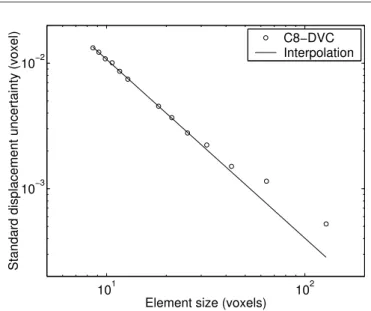
volume g is thus obtained without displacement. A C8-DVC correlation is performed to register the volumes for different element sizes. The measured displacement is ex-pected to be identically zero. Figure 1 shows the standard deviation of the measured
displacements. In all the results reported herein, it was checked that the bias (or av-erage displacement error) was at least one order of magnitude lower than the standard deviation. Consequently, only the latter is shown. This result is in accordance with the resolution analysis performed above. As the element size increases, the displace-ment uncertainty decreases. When extrapolated to small eledisplace-ment sizes, the standard displacement uncertainty reaches levels that make any measurement meaningless and eventually impossible (i.e., matrix [M] is no longer invertible).
A power law interpolation of the standard displacement uncertainty σu = B/`α
describes very well the results for which a significant amount of degrees of freedom does not belong to any edge of the ROI. For the latter, the sensitivity to noise is higher since part of the information is missing (e.g., one half for faces, three fourth for edges, and seven eighth for corners). For element sizes less than 32 voxels, a value α = 1.42 is found, which is in good agreement with the predicted value (1.5) given in Equation (12).
2.2 Regularized DVC
The previous results show that the smaller the element size `, the larger the standard displacement uncertainty. Consequently, if a voxel-scale determination of the displace-ment field is sought, additional information is needed to regularize the measuredisplace-ment problem. This will be achieved by using the equilibrium gap method.
2.2.1 Equilibrium Gap
To enforce mechanical admissibility in an FE sense, the equilibrium gap is first intro-duced. If linear elasticity applies, the equilibrium equations read
[K]{u} = {f} (13)
where [K] is the stiffness matrix, and {f} the vector of nodal forces. When the dis-placement {u} is prescribed and if the (unknown) stiffness matrix is not the true one,
load residuals {fr} will arise
{fr} = [K]{u} − {f} (14)
In the absence of body forces, interior nodes are free from any external load. Conse-quently, the minimization of the equilibrium gap consists in minimizing the following quantity
Φ2m=1
2{u}
t
[K]t[K]{u} (15)
wheretis the transposition operator, and 2Φ2mcorresponds to the sum of the squared
norm of all equilibrium gaps at each interior node. It is worth noting that the unknowns are related to the components of the stiffness matrix. As such, the determination of stiff-ness fields requires a discretization that is coarser than that of the kinematic mesh [44]. However, if the local stiffness can be related to the gray level, then the problem can be regularized, as was shown when identifying a damage law [39]. The same type of procedure will be followed in the sequel, pushing the procedure down to its ultimate limit, namely, the voxel size.
2.2.2 Regularized Correlation Procedure
To solve the coupled minimization of correlation residuals (Φ2c) and equilibrium gap
(Φ2m), a weighted sum of both residuals is defined as
Φ2t= (1 − β) eΦ2m+ β eΦ2c (16)
where β is a dimensionless parameter in the interval [0, 1], eΦ2
mthe normalized
equilib-rium gap, and eΦ2c the normalized correlation residual.
To normalize both residuals, let us consider a unitary displacement field
u1=
u
kuk (17)
With the previous definition, both residuals read g ϕm2≡ Φ2m(u1) = 1 2{u1} t[K]t [K]{u1} f ϕc2≡ Φ2c(u1) = 1 2{u1} t [M]{u1} (18)
The latter values are thus used to make their corresponding residuals dimensionless
and comparable. It is worth noting that any displacement field u1may be used in the
present normalization technique. In the following, a simple “plane wave” displacement is chosen in the x direction with a 16-pixel wavelength (short enough to fit in small
volumes, large enough to avoid discretization artifacts), meaning that with β = 1
2, the
“cut-off wavelength” is equal to 16 pixels. The normalized residuals then read e Φm= Φm e ϕm and eΦc= Φc e ϕc (19)
When the material parameters are known, the minimization of Φ2t with respect to the
unknown degrees of freedom can be performed [41]. It corresponds to an integrated way of measuring displacement fields since the displacement field will satisfy equilibrium equations in addition to the texture conservation.
2.2.3 Regularization of the boundary conditions
The above introduced equilibrium gap functional exploits the residual body forces at
interiornodes, which are to be as small as possible. However, along the boundary of
the ROI neither static nor kinematic information is available. Any displacement field
prescribed on the boundary gives rise to one displacement field for which Φm = 0.
Hence, without boundary conditions, the mechanical regularization vanishes on the former. Similarly, close to the edges, the DVC algorithm gives rise to a higher level of uncertainty than in the bulk, because of the fewer number of neighboring elements. Hence, although regularization is achieved in the bulk, boundaries remain a weak point in the analysis, and as smaller and smaller element sizes down to the elementary voxel are sought, ill-posedness of the problem remains. This observation calls for a third regularization for boundary nodes.
Since no mechanical information is available, it is proposed to introduce a penal-ization of short wavelength displacement fluctuations along the faces of the region of interest. The third objective function to be considered should however vanish for any rigid body motion. It is therefore proposed to introduce
Φ2b= 1
2{u}
t[L]t
where L is a discretized Laplacian operator acting on the faces of the ROI. For any translation and rotation, the above functional vanishes. Let us note that in two dimen-sions, where the same procedure can be applied, the boundary regularization takes the form of the quadratic norm of the second derivative of the displacement field along the edges. In the special case where the boundary of the ROI meets a free surface, a
complete static information (zero tractions: σσσ.n = 0) is available and should be used
instead of the above form.
As for the above cases, the boundary objective function is normalized based on a similar reference displacement field
e Φb= Φb e ϕb (21)
where fϕb2≡ Φ2b(u1) = (1/2){u1}t[L]t[L]{u1}. Finally, the total objective function to
be minimized reads
Φ2t = (1 − β − γ) eΦ2m+ β eΦ2c+ γ eΦ2b (22)
where β > 0, γ > 0 and β + γ < 1.
2.2.4 Justification of the regularization
To understand that the above combination of the correlation and mechanical resid-uals will allow for a regularization, it is necessary to resort to a spectral analysis of both functionals. Let us consider a displacement field in the form of a plane wave
du(x) = du0exp(ik.x) with a vanishing amplitude |du0| as a perturbation of a
refer-ence displacement field, ueq ideally assumed to minimize both functionals. The
corre-lation residual amounts to
Φ2c(ueq+ du) = Φ2c(ueq) +1
2{du}
t
[M]{du} (23)
On average, the residual perturbation dΦ2c scales as |du0|2h[M]i|Ω| The important
feature to note is that this term is independent of the wavevector k.
The mechanical residual perturbation is also a quadratic form in du0. However, it
scales as the fourth power of the wavenumber
A similar spectral analysis performed on the boundary term shows that the scaling of
Φbfor a plane wave displacement field is similar to that of the mechanical regularization
dΦ2b ∝ |k|4|du0|
2
|∂Ω| (25)
where ∂Ω is the outer boundary of the considered ROI. Hence, Φmand Φbare natural
complements.
Balancing the expressions of Φcand Φmor Φbshows that there are two
character-istic length scales, ξ and ξb, such that
ξ ∝ 4 s 1 − β − γ β and ξb∝ 4 r γ β (26)
where ξbgives the depth of the boundary layer that is affected by the boundary
regu-larization. Concerning the bulk, below the ξ length scale, Φm dominates over Φc, and
hence the small scale displacement is mechanically admissible, whereas at large length scales the correlation residual is dominant. These two length scales play the same role in terms of regularization as the mesh size in the C8-DVC formulation. However, rather than choosing finite element shape functions, which are convenient but not mechani-cally significant, the introduced formulation implements, in addition to a conventional boundary regularization, a physically motivated short scale regularization where the information is available (i.e., in the bulk). Adjusting the value of the parameters β and γ is a way of tuning the regularization scales.
3 Artificial Cases
Two artificial cases are studied, namely, the first one whose texture has a low frequency content. The second one is directly related to the practical case that will be studied in Section 4.
3.1 First case
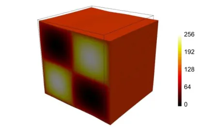
The deformation of an artificial isotropic material with slowly varying Young’s modulus E is first analyzed. As shown in Figure 2, Dirichlet boundary conditions are prescribed
to solve a regular 3D finite element problem, which allows then to generate a deformed image. In the present case uniform displacements corresponding to an average uniaxial strain of 1% are prescribed on two opposite faces, and the other external boundaries are traction-free. This synthetic case is considered in order to validate the method. The
dimensionlesscorrelation residual, η, is defined as
η ≡ 1 max f − min f s 1 |Ω| X x (f (x + u(x)) − g(x))2 (27)
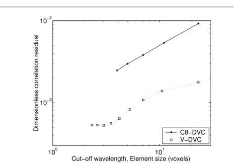
Figure 3 shows the change of the dimensionless correlation residual for two different DVC techniques as a function of a regularization length scale. The first curve is a reference solution where a global C8-DVC is chosen. In that case, the regularization length scale ξ is taken as the element size `. The increase of the residual is due to a systematic error caused by the fact that coarser and coarser elements cannot capture accurately the actual displacement field. It is to be stressed that for ` < 4 voxels the C8-DVC algorithm becomes unstable (see Figure 1). The second curve corresponds to the present mechanical regularization using homogeneous elastic properties. In that
case, ξb is set to 16 voxels. The correlation residual typically is cut down by a factor
of 4. Moreover, ξ can be reduced to values as small as 2 voxels with no convergence problems.
The robustness of the proposed method is better than that achieved with a standard C8-DVC procedure. It is worth noting that the correlation residual is lower even if the material properties are not the actual ones.
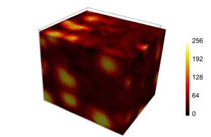
3.2 Second case
The texture that is used in this example (Figure 4) was obtained from a X-Ray tomog-raphy (for a more detailed description, see Section 4). The goal of this example is to study a case that is more realistic in terms of texture.
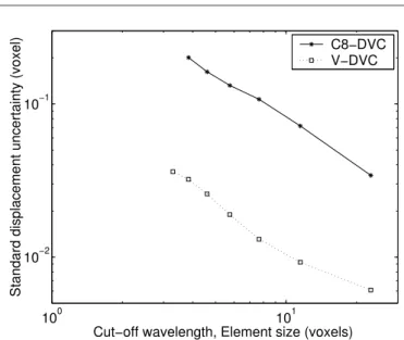
The effect of noise is shown in Figure 5 with the proposed (V-DVC) approach and with C8-DVC. The same procedure as in Section 2 is followed. The standard displacement uncertainty is lowered by one order of magnitude when comparing
C8-DVC and V-C8-DVC. This result shows that the proposed regularization is very effective, even for low cut-off lengths. Since the V-DVC approach also leads to smaller correlation residuals, it means that V-DVC is not a tradeoff between stability and accuracy. In the
present case, a small ROI (i.e., 233voxels) was considered since voxel-scale calculations
are performed. Consequently, edge effects dominate and the power −3/2 expected from Equation (12) is not found. Rather, a power −1 is observed suggesting that face boundaries are the main source of uncertainty.
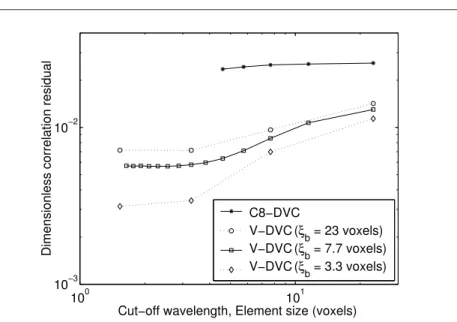
The deformation of the considered texture is now analyzed. As previously, the local Young’s modulus E is assumed to be a deterministic function of the gray level (an affine variation is chosen with a maximum contrast of 3 over the gray levels spanned by the reference volume, namely, the maximum value is equal to three times the minimum value of E). An elastic computation is first performed when a 1%-extension along the x-direction is prescribed as in the previous case. The lateral faces are stress-free, and the displacement field is used to create an artificial deformed volume. The change of the dimensionless correlation residual as a function of the regularization length scale is shown in Figure 6 for the two different DVC techniques. All the trends observed in the previous case are also found for the present texture. In particular, a significant reduction of correlation residuals is achieved with the regularization, especially for small regularization lengths. A factor 4 gain is again observed. As in the previous case, a saturation of the correlation residuals occurs for small regularization lengths, ξ, signaling that the results become independent of that parameter. The main difference is related to the absolute levels themselves that are higher in the present case. This is due to the more rapidly varying displacement field induced by the more complex texture.
Further, it is shown that as the cut-off wavelength ξb decreases, the correlation
residuals decrease as well. This result allows to regularize the measurement problem with very small wavelengths for the boundary conditions. The fact that a plateau
region when ξ < 4 voxels is observed for any tested values of ξballows for a choice of ξ
used for the boundary conditions, ξbhas a slightly different role, namely, in the generic
case (when the displacement close to the boundaries has to be considered) it should be as low as possible, but high enough to maintain the global convergence properties. From the study of these two artificial cases, it appears that the proposed regu-larization fulfills the expected objective. It allows for a rapid convergence towards a displacement field that has a much lower residual level than what could be achieved traditionally. Moreover, it has been shown that for low ξ values, the residuals ap-peared to become independent of ξ. This means that the regularization is neutral and only provides a way of interpolating the displacement at small scales when another (correlation-based) information is missing, thus preserving the well-posedness of the problem, without compromise to the image registration algorithm.
4 Practical Case
The material studied herein is a ferritic cast iron whose composition is 3.4 wt.% C, 2.6 wt.% Si, 0.05 wt.% Mg, 0.19 wt.% Mn, 0.005 wt.% S and 0.01 wt.% P. After casting
and heat treatment (ferritization at 880 ◦C, followed by air cooling) the
microstruc-ture obtained is a ferritic matrix (98 wt.% ferrite and 2 wt.% perlite, average grain size 50 µm) with a 14% volume fraction of graphite nodules. Carbon (nodules) and iron (matrix) have atomic numbers that are different enough to give a strong X-ray attenuation contrast. Therefore, the spherical nodules, which are homogeneously dis-tributed inside the matrix, are easily imaged by tomography and they can be used as natural markers for image correlation in the reconstructed 3-D images. The average nodule diameter of 45 µm is large enough to allow for a relatively low resolution voxel size to be used for tomography. This also enables one to observe millimetric samples, the only limitation for the sample size being the overall attenuation of the material that has to allow for, at least, 10% transmission of the incoming X-Ray beam.
The experiment was performed at the European Synchrotron Radiation Facility (ESRF) in Grenoble (France) on Beamline ID19. The synchrotron beam is parallel so that the voxel size only depends on the optics used. To obtain a 3D image of
the specimen, six hundred radiographs (referred to as a scan) were recorded while
the sample was rotating over 180◦ along a vertical axis. A Fast Readout Low Noise
(FReLoN) 14-bit CCD camera with a resolution of 2048 × 2048 pixels was used [45]. The time required to acquire each image was set to 3 s, resulting in a total scan time of about 42 minutes.
A specially designed in situ fatigue testing machine that allows for loading and cycling (up to a frequency of 50 Hz) of the specimen [46] was used. The specimen was loaded to a maximum level of 273 N, and then unloaded. Five tomographic scans were acquired during which the load level was equal to 22, 150, 200, 250 and 273 N, and one scan upon unloading (load level: 21 N). In the following, only the scan correspond-ing to the maximum load level will be considered in addition to the reference scan. Reconstruction of the tomographic data was performed with a conventional filtered back-projection algorithm [47]. It provides a reconstructed volume with a 32-bit dy-namic range that is proportional to the local attenuation coefficient. The 32-bit volume is subsequently re-encoded onto an 8-bit range to reduce data size and computation time. This truncation does not degrade significantly the raw data since reconstruction artifacts are of higher amplitude than the error induced by the former [37, 38]. The region of interest has dimensions of 200 × 340 × 512 voxels, i.e., with a voxel size of
5.06 µm in the reconstructed images, 1.01 × 1.72 × 2.59 mm3.
Numerical tests are analyzed on a ROI in the center of the volume of size 23 × 23 × 23 supervoxels (i.e., 13, 824 × 3 degrees of freedom for a V-DVC approach) after a pyramidal filter is applied (i.e., a recursive construction that consists in averaging
groups of 2×2×2 voxels to form a “super-voxel”). The lengths ξb and ξ are initially set
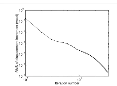
to 16 supervoxels. In the present case, the physical size of each considered (super)voxel (or element since V-DVC is used) is equal to 10.12 µm. This coarsening was necessary since the nodule spacing was too big to get a sufficiently rich texture. A first step was applied to correct for rigid body translations (up to a level of 19.5 supervoxels along the loading direction). Then the V-DVC procedure itself is run. The convergence in
terms of displacement corrections is shown in figure 7; a rather fast rate is observed. The total CPU time is equal to 15 min on a Core i7 (2.9 GHz) computer.
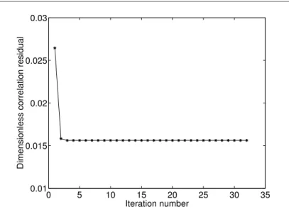
The next check is given by the correlation residual that measures the registration quality. Figure 8 shows that there is a change only for the first three iterations.
After-wards, for ξband ξ both equal to 16 voxels, a saturation is observed at a level of 1.6 %
of the dynamic range. This value is significantly lower than previously observed with C8-DVC [26, 28] and reaches values commonly observed in Q4-DIC [33]. The fact that the dimensionless residuals tend to such low values is an additional indication that
the results are trustworthy. This value can be further decreased down to 1 % when ξb
and ξ are set to 6 voxels. In comparison, the correlation residual that was obtained with the C8-DVC approach on the same ROI is equal to 3 % when 9 elements are used, meaning that while improving the robustness, V-DVC allows for decrease of the correlation residual by a factor of 3. This result further validates the V-DVC approach.
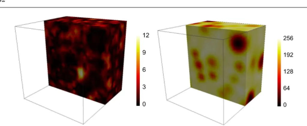
The correlation residual map is shown in Figure 9 when ξband ξ are set to 6 voxels.
The maximum value is equal to 12 gray levels for a dynamic range of the scans of 256 gray levels. Except at very few locations, the residual levels are very low everywhere. This may indicate deviations from the assumed behavior or a small texture gradient that does not allow for a good (local) registration. The scan g corresponding to the deformed state is given in the same figure for comparison purposes. The location of the nodules generally disappears in the correlation residual map.
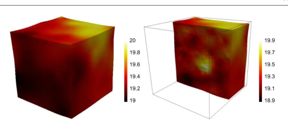
Figure 10 shows the deformed volume at convergence of the V-DVC procedure. A smooth displacement field is observed on the external surface. This result is made
possible by the use of the wavelength ξb. The displacement field is also regular inside the
volume as can be seen on the cut shown in Figure 10 for the displacement component along the tensile direction. It is worth emphasizing that the overall amplitude of the displacement field over the analyzed volume is equal to 1 voxel, or 10 µm. To see more clearly the impact of boundary and bulk regularization, Figure 10 also shows the component of the displacement along the tensile direction in the mid section of the volume. The corresponding texture as well as the correlation residual field of the
same section are shown for comparison purposes in Figure 9. It is worth remembering that the displacement fluctuations are due to the heterogeneous nature of the studied material at the voxel scale.
5 Conclusion
A new regularized Digital Volume Correlation method was introduced herein. It allows for the measurement of displacements at a voxel level, exploiting the assumption of an elastic behavior at a small scale, and a boundary regularization. When such a regularization is not used, even global DVC is not reliable for small element sizes, and eventually does not converge for very small element sizes since the problem becomes ill-posed. The regularization is performed using the Equilibrium Gap Method.
The correlation residuals are extremely small (much smaller than using a global DVC algorithm for any element size) showing the ability of the method to provide a faithful (and mechanically admissible) displacement field. To further lower the residu-als, the measurement technique contains an “on the fly” identification procedure, which was not used herein. It consists in considering the elastic parameters as unknowns to be determined as was proposed for 2D applications [40]. A first step will consist in evaluating the sensitivity of the measurement technique to the sought mechanical pa-rameters.
Acknowledgments
This work was funded under the grant ANR-09-BLAN-0009-01 (RUPXCUBE Project). It was also made possible by an ESRF grant for the experiment MA-501 on beam-line ID19. The scans were obtained with the help of Drs. J.-Y. Buffi`ere, A. Gravouil, N. Limodin, W. Ludwig, and J. Rannou.
References
1. Baruchel J, Buffi`ere J-Y, Maire E, Merle P, Peix G. X-Ray Tomography in Material Sci-ences. Hermes Science: Paris (France); 2000.
2. Maire E, Buffi`ere J-Y, Salvo L, Blandin J-J, Ludwig W, L´etang J-M. On the application of X-ray microtomography in the field of materials science. Adv. Eng. Mat. 2001; 3(8):539-546.
3. Bernard D, eds. 1st Conference on 3D-Imaging of Materials and Systems 2008. ICMCB: Bordeaux (France), 2008.
4. Stock SR. MicroComputed Tomography: Methodology and Applications. CRC; 2008. 5. Stock SR. Recent advances in X-Ray microtomography applied to materials. Int. Mat.
Rev. 2008; 53(3):129-181.
6. Banhart J. Advanced Tomographic Methods in Materials Research and Engineering. Ox-ford University Press; 2008.
7. Bart-Smith H, Bastawros A-F, Mumm DR, Evans AG, Sypeck DJ, Wadley HNG. Com-pressive deformation and yielding mechanisms in cellular Al alloys determined using X-ray tomography and surface strain mapping. Acta Mater. 1998; 46(10):3583-3592.
8. Babout L, Maire E, Buffi`ere J-Y, Foug`eres R. Characterisation by X-Ray computed tomog-raphy of decohesion, porosity growth and coalescence in model metal matrix composites. Acta Mater. 2001; 49(11):2055-2063.
9. Bontaz-Carion J, Pellegrini Y-P. X-Ray Microtomography Analysis of Dynamic Damage in Tantalum. Adv. Eng. Mat. 2006; 8(6):480-486.
10. Schilling PJ, Karedla BR, Tatiparthi AK, Verges MA, Herrington PD. X-ray computed microtomography of internal damage in fiber reinforced polymer matrix composites. Comp. Sci. Tech. 2005; 65(14):2071-2078.
11. Sinclair R, Preuss M, Maire E, Buffiere J-Y, Bowen P, Withers PJ. The effect of fibre frac-tures in the bridging zone of fatigue cracked Ti6Al4V/SiC fibre composites. Acta Mater. 2004; 52(6):1423-1438.
12. Ferri´e E, Buffiere J-Y, Ludwig W, Gravouil A, Edwards L. Fatigue crack propagation: In situ visualization using X-ray microtomography and 3D simulation using the extended finite element method. Acta Mat. 2006; 54(4):1111 -1122.
13. Wolfsdorf TL, Bender WH, Voorhees PW. The morphology of high volume fraction solid-liquid mixtures: An application of microstructural tomography. Acta Mater. 1997; 45(6):2279-2295.
14. Ludwig O, Dimichiel M, Salvo L, Su´ery M, Falus P. In-situ Three-Dimensional Microstruc-tural Investigation of Solidification of an Al-Cu Alloy by Ultrafast X-ray Microtomography. Metall. Mat. Trans. A 2005; 36(6):15151523.
15. Maire E, Colombo P, Adrien J, Babout L, Biasetto L. Characterization of the morphology of cellular ceramics by 3D image processing of X-ray tomography. J. Eur. Ceram. Soc. 2007; 27:1973-1981.
16. Viot P, Bernard D. Impact test deformations of polypropylene foam samples followed by microtomography. J. Mater. Sci. 2006; 41:1277-1279.
17. Ludwig W, Buffi`ere J-Y, Savelli S, Cloetens P. Study of the interaction of a short fatigue crack with grain boundaries in a cast Al alloy using X-ray microtomography. Acta Mater. 2003; 51(3):585-598.
18. Youssef S, Maire E, Gaertner R. Finite element modelling of the actual structure of cellular materials determined by X-ray tomography. Acta Mater. 2005; 53(3):719-730.
19. Maire E, Fazekas A, Salvo L, Dendievel R, Youssef S, Cloetens P, Letang JM. X-ray tomography applied to the characterization of cellular materials. Related finite element modeling problems. Comp. Sci. Tech. 2003; 63(16):2431-2443.
20. Nielsen SF, Poulsen HF, Beckmann F, Thorning C, Wert JA. Measurements of plastic displacement gradient components in three dimensions using marker particles and syn-chrotron X-ray absorption microtomography. Acta Mater. 2003; 51(8):2407-2415. 21. Toda H, Sinclair I, Buffi`ere J-Y, Maire E, Connolley T, Joyce M, Khor KH, Gregson P.
As-sessment of the fatigue crack closure phenomenon in damage-tolerant aluminium alloy by in-situ high-resolution synchrotron X-ray microtomography. Phil. Mag. 2003; 83(21):2429-2448.
22. Withers PJ, Bennett J, Hung Y-C, Preuss M. Crack opening displacements during fatigue crack growth in Ti-SiC fibre metal matrix composites by X-ray tomography. Mat. Sci. Technol. 2006; 22(9):1052-1058.
23. Bay BK, Smith TS, Fyhrie DP, Saad M. Digital volume correlation: three-dimensional strain mapping using X-ray tomography. Exp. Mech. 1999; 39:217-226.
24. Bornert M, Chaix J-M, Doumalin P, Dupr´e J-C, Fournel T, Jeulin D, Maire E, Moreaud M, Moulinec H. Mesure tridimensionnelle de champs cin´ematiques par imagerie volumique pour l’analyse des mat´eriaux et des structures. Inst. Mes. M´etrol. 2004; 4:43-88. 25. McKinley TO, Bay BK. Trabecular bone strain changes associated with subchondral
stiff-ening of the proximal tibia. J. Biomech. 2003; 36(2):155163.
26. Roux S, Hild F, Viot P, Bernard D. Three dimensional image correlation from X-Ray computed tomography of solid foam. Comp. Part A 2008; 39(8):1253-1265.
27. R´ethor´e J, Tinnes J-P, Roux S, Buffi`ere J-Y, Hild F. Extended three-dimensional digital image correlation (X3D-DIC). C. R. M´ecanique 2008; 336:643-649.
28. Hild F, Maire E, Roux S, Witz J-F. Three dimensional analysis of a compression test on stone wool. Acta Mat. 2009; 57:3310-3320.
29. Limodin N, R´ethor´e J, Buffi`ere J-Y, Gravouil A, Hild F, Roux S. Crack closure and stress intensity factor measurements in nodular graphite cast iron using 3D correlation of laboratory X ray microtomography images. Acta Mat. 2009; 57(14):4090-4101.
30. Limodin N, R´ethor´e J, Buffi`ere J-Y, Hild F, Roux S, Ludwig W, Rannou J, Gravouil A. Influence of closure on the 3D propagation of fatigue cracks in a nodular cast iron investigated by X-ray tomography and 3D Volume Correlation. Acta Mat. 2010; 58:2957-2967.
31. Rannou J, Limodin N, R´ethor´e J, Gravouil A, Ludwig W, Ba¨ıetto-Dubourg M-C, Buffi`ere J-Y, Combescure A, Hild F, Roux S. Three dimensional experimental and numerical mul-tiscale analysis of a fatigue crack. Comp. Meth. Appl. Mech. Eng. 2010; 199:1307-1325. 32. Bergonnier S, Hild F, Roux S. Digital image correlation used for mechanical tests on
crimped glass wool samples. J. Strain Analysis 2005; 40(2):185-197.
33. Besnard G, Hild F, Roux S. “Finite-element” displacement fields analysis from digital images: Application to Portevin-Le Chatelier bands. Exp. Mech. 2006; 46:789-803. 34. Bornert M, Br´emand F, Doumalin P, Dupr´e J-C, Fazzini M, Gr´ediac M, Hild F, Mistou
S, Molimard J, Orteu J-J, Robert L, Surrel Y, Vacher P, Wattrisse B. Assessment of Digital Image Correlation measurement errors: Methodology and results. Exp. Mech. 2009; 49(3):353-370.
35. R´ethor´e J, Hild F, Roux S. Shear-band capturing using a multiscale extended digital image correlation technique. Comp. Meth. Appl. Mech. Eng. 2007; 196(49-52):5016-5030. 36. R´ethor´e J, Hild F, Roux S. Extended digital image correlation with crack shape
optimiza-tion. Int. J. Num. Meth. Eng. 2008; 73(2):248-272.
37. Davis GR, Elliot JC. Artefacts in X-ray microtomography of materials. Mat. Sci. Eng. 2006; 22(9):1011-1018.
38. Ketcham RA. New algorithms for ring artefact removal. Developments in X-Ray Tomog-raphy V , Bonse U, eds. SPIE: Bellingham Wa, 2006; 00-1-15.
39. Roux S, Hild F. Digital Image Mechanical Identification (DIMI). Exp. Mech. 2008; 48(4):495-508.
40. Leclerc H, P´eri´e J-N, Roux S, Hild F. Integrated Digital Image Correlation for the Identifi-cation of Mechanical Properties. MIRAGE 2009 , Gagalowicz A, Philips W, eds. Springer-Verlag: Berlin (Germany), 2009; LNCS 5496:161-171.
41. R´ethor´e J, Roux S, Hild F. An extended and integrated digital image correlation technique applied to the analysis fractured samples. Eur. J. Comput. Mech. 2009; 18:285-306. 42. Claire D, Hild F, Roux S. A finite element formulation to identify damage fields: The
equilibrium gap method. Int. J. Num. Meth. Engng. 2004; 61(2):189-208.
43. Roux S, Hild F. Stress intensity factor measurements from digital image correlation: post-processing and integrated approaches. Int. J. Fract. 2006; 140(1-4):141-157.
44. Roux S, Hild F. From image analysis to damage constitutive law identification. NDT.net 2006; 11(12):roux.pdf.
45. Labiche J-C, Mathon O, Pascarelli S, Newton MA, Guilera Ferre G, Curfs C, Vaughan G, Homs A, Carreiras DF. The fast readout low noise camera as a versatile X-ray detector for time resolved dispersive extended X-ray absorption fine structure and diffraction studies of dynamic problems in materials science, chemistry and catalysis. Rev. Sci. Instrum. 2007; 78:091301.
46. Buffi`ere J-Y, Ferri´e E, Proudhon H, Ludwig W. Three-dimensional visualisation of fatigue cracks in metals using high resolution synchrotron X-ray micro-tomography. Mat. Sci. Tech. 2006; 22(9):1019-1024.
47. Kak AC, Slaney M. Principles of Computerized Tomographic Imaging. Society of Indus-trial and Applied Mathematics; 2001.
List of Figures
1 Standard displacement uncertainty as a function of the element size `
in C8-DVC. The interpolation (solid line) is described by a power law
B/`α, where α = 1.42 is good agreement with Equation (12). . . 24
2 Deformed state of the artificial material used to generate a slowly varying
texture. The gray level is a growing affine function of the local Young’s modulus that varies from 1 to 100. The frame depicts the edges of the
undeformed volume. . . 25
3 Dimensionless correlation residual, η, with two DVC methods as a
func-tion of finite element sizes, `, for C8-DVC, and of cut-off wavelengths, ξ, for the proposed V-DVC method. The C8-DVC curve was stopped at
the left because of lack of convergence. . . 26
4 Deformed state of material used for the second test case. The gray level
is a growing affine function of the local Young’s modulus that ranges
from 1 to 3. The frame depicts the edges of the undeformed volume. . 27
5 Standard displacement uncertainty as a function of the element size ` in
C8-DVC, and the cut-off length ξ when ξb= 16 voxels for V-DVC. . . . 28
6 Dimensionless correlation residual, η, with two DVC methods as a
func-tion of finite element sizes for C8-DVC, and cut-off wavelengths for the proposed V-DVC method. The C8-DVC curve was stopped at the left
because of lack of convergence. . . 29
7 Convergence of the present method in terms of RMS of the
displace-ment incredisplace-ment between two iterations, as a function of the number of iterations for the chosen ferritic cast iron tomographies (load levels: 22
and 273 N). . . 30
8 Dimensionless correlation residuals as a function of the number of
iter-ations for the chosen ferritic cast iron tomographies (load levels: 22 and
9 Correlation residual map (left) and deformed scan (right) when ξb and
ξ are set to 6 voxels. Note that the dynamic range of the residual map is significantly lower than that of the deformed scan (256 gray levels).
The frame depicts the edges of the undeformed volume. . . 32
10 Deformed volume with displacement amplitude (left) and along the
ten-sile direction (right) expressed in voxels when ξband ξ are set to 6 voxels.
101 102 10−3
10−2
Element size (voxels)
Standard displacement uncertainty (voxel)
C8−DVC Interpolation
Fig. 1 Standard displacement uncertainty as a function of the element size ` in C8-DVC. The interpolation (solid line) is described by a power law B/`α
, where α = 1.42 is good agreement with Equation (12).
256
192
128
64
0
Fig. 2 Deformed state of the artificial material used to generate a slowly varying texture. The gray level is a growing affine function of the local Young’s modulus that varies from 1 to 100. The frame depicts the edges of the undeformed volume.
100 101 10−3
10−2
Cut−off wavelength, Element size (voxels)
Dimensionless correlation residual C8−DVC
V−DVC
Fig. 3 Dimensionless correlation residual, η, with two DVC methods as a function of finite element sizes, `, for C8-DVC, and of cut-off wavelengths, ξ, for the proposed V-DVC method. The C8-DVC curve was stopped at the left because of lack of convergence.
256
192
128
64
0
Fig. 4 Deformed state of material used for the second test case. The gray level is a growing affine function of the local Young’s modulus that ranges from 1 to 3. The frame depicts the edges of the undeformed volume.
100 101 10−2
10−1
Cut−off wavelength, Element size (voxels)
Standard displacement uncertainty (voxel)
C8−DVC V−DVC
Fig. 5 Standard displacement uncertainty as a function of the element size ` in C8-DVC, and the cut-off length ξ when ξb= 16 voxels for V-DVC.
100 101 10−3
10−2
Cut−off wavelength, Element size (voxels)
Dimensionless correlation residual
C8−DVC V−DVC(ξb = 23 voxels) V−DVC(ξb = 7.7 voxels) V−DVC(ξb = 3.3 voxels)
Fig. 6 Dimensionless correlation residual, η, with two DVC methods as a function of finite element sizes for C8-DVC, and cut-off wavelengths for the proposed V-DVC method. The C8-DVC curve was stopped at the left because of lack of convergence.
100 101 10−6 10−5 10−4 10−3 10−2 10−1 100 Iteration number
RMS of displacement increment (voxel)
Fig. 7 Convergence of the present method in terms of RMS of the displacement increment between two iterations, as a function of the number of iterations for the chosen ferritic cast iron tomographies (load levels: 22 and 273 N).
0 5 10 15 20 25 30 35 0.01 0.015 0.02 0.025 0.03 Iteration number
Dimensionless correlation residual
Fig. 8 Dimensionless correlation residuals as a function of the number of iterations for the chosen ferritic cast iron tomographies (load levels: 22 and 273 N).
12 9 6 3 0 256 192 128 64 0
Fig. 9 Correlation residual map (left) and deformed scan (right) when ξband ξ are set to
6 voxels. Note that the dynamic range of the residual map is significantly lower than that of the deformed scan (256 gray levels). The frame depicts the edges of the undeformed volume.
20 19.8 19.6 19.4 19.2 19 19.9 19.7 19.5 19.3 19.1 18.9
Fig. 10 Deformed volume with displacement amplitude (left) and along the tensile direction (right) expressed in voxels when ξband ξ are set to 6 voxels. The frame depicts the edges of