HAL Id: hal-00527541
https://hal.archives-ouvertes.fr/hal-00527541
Submitted on 8 Jul 2018
HAL is a multi-disciplinary open access
archive for the deposit and dissemination of
sci-entific research documents, whether they are
pub-lished or not. The documents may come from
teaching and research institutions in France or
abroad, or from public or private research centers.
L’archive ouverte pluridisciplinaire HAL, est
destinée au dépôt et à la diffusion de documents
scientifiques de niveau recherche, publiés ou non,
émanant des établissements d’enseignement et de
recherche français ou étrangers, des laboratoires
publics ou privés.
Relationship between physical and subspace propagation
channels
Patrice Pajusco, Nadine Malhouroux-Gaffet
To cite this version:
Patrice Pajusco, Nadine Malhouroux-Gaffet. Relationship between physical and subspace propagation
channels. PIMRC 2010 : 21st Annual IEEE International Symposium on Personal, Indoor and Mobile
Radio Communications, Sep 2010, Istanbul, Turkey. �hal-00527541�
Relationship between physical and
subspace propagation channels
Simulation and experimental study
Patrice Pajusco
Lab-STICC, CS 83818 Telecom Bretagne Brest, France [email protected]Nadine Malhouroux-Gaffet
Orange Labs Belfort, France [email protected]Abstract— The channel capacity of a MIMO telecommunication system depends on different parameters such as the signal-to-noise ratio, the space-time characteristics of the propagation channel, the antenna array geometry and the antenna pattern. However, the propagation channel remains the strongest constraint imposed on designers of new radio air interfaces. Using a MIMO channel model, computer simulations are performed to highlight the relation between the radiation pattern of subspace channels and the physical space-time characteristics of the propagation channel. This provides a better understanding of the subspace channel origins and achievability of degrees of freedom. In addition to the simulation approach, UWB MIMO channel measurements are used. Both simulation and experimental results show that there is not a bijective relation between physical paths and subspace channels. The number of subspace channels is the same but the amplitudes and directions can be different, leading to inaccuracies in the space-time characteristics of the propagation channel. Nevertheless, the results are promising for fast-jointed DoA-DoD channel estimation.
I. INTRODUCTION
The channel capacity of MIMO communication systems depends on different parameters, such as the signal-to-noise ratio, the space-time characteristics of the propagation channel, the antenna array geometry and the antenna patterns. Among all of these elements, only the propagation channel cannot be optimized by air interface designers. As Bonek highlights in [1], it is essential to thoroughly understand the subjacent phenomena in order to provide reliable models and conclusions. The aim of this article is to investigate the relationship between the physical properties of propagation channels and the subspace propagation channels obtained by the singular decomposition of the MIMO transmission radio channel. This study will allow an improvement in the definition and the understanding of the origin of the maximum capacity of MIMO communication systems.
Simulations were performed to highlight the relationship between the radiation pattern associated with each eigenmode and the space-time characteristics of the propagation channel. This study is important for engineering and simulation studies. Indeed, in a MIMO communication, the power transmitted over subspace channels generates a radiation pattern which is no longer omnidirectional. The prediction of radio coverage and
interference is no longer related only to the antenna pattern, but also to the spatial characteristics of the propagation channel. This study will also provide a better physical understanding of the subspace channels’ origin, their associated MIMO capacity and the corresponding degrees of freedom of the propagation channel. To complete the simulation study, an experimental MIMO UWB campaign was carried out. It is based on a measurement technique that is able to investigate the 3D space-time characteristics of a real channel [2]. Results obtained in an indoor environment will be presented and analyzed.
II. DEFINITIONS
A. Transmission and Propagation Channel
First, it is important to define the transmission channel and the propagation channel. A SISO transmission channel can be seen as a two-port network formed by the two antenna extremities of the radio link. The transfer function can be easily obtained by using, for example, a vector network analyzer. The concept of the propagation channel is more abstract because its characteristics cannot be directly measured. It can be simply defined as the transmission channel without the antenna effects.
B. MIMO Channel
A MIMO system is defined as a transmission system with
T
n transmitter antennas and n receiver antennas. In a R
narrowband context, the propagation channel can be represented by a complex matrix H of dimension nR×nT .
Each element h of the matrix H represents the complex i j,
transmission gain between the receiving antenna i and the transmitting antenna j. X is the vector corresponding to the transmitted signals applied to the emitter antenna; Y is the vector corresponding to the received signals. In a noise-free configuration, the received signal is expressed as:
Y = HX (1)
By using singular value decomposition (SVD) the matrix
H
can be expressed as:{ }
1with b and =rank( )
H
i i
diag λ = b
=
1, ,2 3 nT
v v v v
⎡ ⎤
= ⎣ ⎦
V " : Unitary matrix of nT×nT dimension containing the vectors columns vk of the input basis.
1, ,2 3 nR
u u u u
⎡ ⎤
= ⎣ ⎦
U " : Unitary matrix of nR×nR dimension containing the vectors columns uk of the output basis.
Σ is the diagonal matrix containing the singular values sorted by descending order.
The singular values are positive or null. The nonzero values correspond to the eigenvalues of the matrix HHH, identical to
the nonzero eigenvalues of H HH . Considering X = V X' H
the representation of
X
in the input basis and Y = U Y' -1the representation of
Y
in the output basis, the simplified relation Y' = ΣX is obtained. Σ is diagonal, so the MIMO 'transmission is equivalent to the transmission of parallel links, whose amplitude of each subspace channel K is given by
Σ
k ,k.Figure 1 shows the two representations respectively Y = HX
and Y' = ΣX'
Figure 1. Physical and subspace representation of a MIMO transmission
C. Channel Capacity
The channel capacity concept was introduced by Shannon in 1948 [3]. In the case of a link between two antennas, the capacity in bit/s/Hz is given by equation 3.
1 2
log (1 + ) .
SISO
C = ρ bps Hz− (3)
With ρ is the signal to noise ratio. This definition highlights two fundamental properties. First, the capacity grows with signal to noise ratio. Secondly, when the signal to noise ratio is large, the increase of capacity will be very slow. The capacity increase of a MIMO system is based on the data rate of the previous subspace channels. The number of channels is directly related to the number of significant eigenvalues of the matrixHHH. So the larger the number of
significant eigenvalues is, the bigger the potential capacity. The total capacity of MIMO system is defined as the sum of the capacity of each subspace channel:
min( , ) 2 1 log 1 T R n n MIMO i i T C nρ λ = ⎛ ⎞ = ⎜ + ⎟ ⎝ ⎠
∑
(4)The capacity will depend on the power allocation strategy on each subspace channel. The optimal solution consists in using the Waterfilling algorithm. However, this solution requires the channel state information at the transmitter which is not always available.
D. Subspace Channel Pattern Radiation
The real and subspace channels in MIMO were recalled in figure 1 in function of X,Y and X',Y'. Considering the Kth
subspace channel which corresponds to the Kth nonzero
singular value of the matrix channel
H
, we have :k k k k k k
y
v
x
u
'
=
Σ
,'
(5) That means that the Kth subspace channel is obtained byweighting the transmitter array by the vector
u'
k and the receiver array by the vectorv'
k. So, the resulted subspace channel will have a gain ofΣ
k ,kand will be orthogonal to the other subspace channels. Using a 3D complex antenna pattern of the array, it is easy to find the physical radiation pattern of this subspace channel. Considering that the antenna pattern of the ith element of the transmitter array is TX(
,)
i
a θ ϕ with the
complex components
e
G
θ ande
G
ϕ of the radiation directions θ and ϕ . Theses diagrams include the spatial configuration of the array. We can also similarly define the radiation pattern( )
,RX i
a θ ϕ of the antenna pattern of the ith element of the
receiver array. The relation between the antenna pattern
(
,)
TX k
A θ ϕ and RX
(
,)
k
A θ ϕ corresponding to the Kth subspace
channel is given by:
(
)
(
)
( )
1 , nT X , ' TX T k i k i A θ ϕ a θ ϕ u i = =∑ × (6)(
)
(
)
( )
1 , nR X , ' RX R k i k i A θ ϕ a θ ϕ v i = =∑ × (7)III. BEHAVIOR OF PHYSICAL AND SUBSPACE CHANNELS
A. Introduction
The matrix
H
of the transmission channel depends on thepropagation phenomena between the transmitter and the receiver, on the characteristics of the antennas and the geometry of the array. There is, a priori, a relation between the physical properties of the propagation channel ie, that is the space-time characteristics of the propagation and the singular value decomposition. Some authors such as Loyka [4] had studied this relation in the case of waves guides. It was, for example, possible to compare the various propagation modes of the wave guide to the modes generated by a MIMO array set in the guide. These results are interesting because each mode of the wave guide can be considered as a plane wave undergoing some reflections. But this study does not represent a typical radio-mobile environment. From MIMO simulations, deeper investigations will be carried out by the evaluation of the directions of arrival and departure.
B. Channel Simulation Principle
The developed channel simulator uses the double directional approach introduced by Steinbauer in [ 5 ]. This allows simulation of the antennas pattern independently of the propagation channel. Thus, the transmission channel can be known whatever the antenna array geometry. Most of the MIMO channel models are based on this formalism (802.11n,
UMTS, Wimax...). The principle consists in modelling the radio channel by a set of multipaths described by their physical characteristics: direction of departure (DoD) direction of arrival (DoA), complex attenuation for each polarization, delay, Doppler. The transmission MIMO channel is then obtained from the characteristics of the multipaths, of the array geometry and the antenna pattern. An efficient and reliable implementation of this model requires optimizations detailed in [ 6 ].
C. Simulation Configuration
The choice of the array geometry is very important. Indeed, most of the MIMO array geometries provide ambiguitie results. For example, the linear array has a conical ambiguity. Thus, two rays coming from different directions are perceived in an identical path by the array and consequently reduce the number of degrees of freedom of the MIMO channel. Circular arrays have been chosen for simulations because they show no ambiguity in azimuth. Simulations are carried out at 5 GHz, corresponding to the band used by WIFI systems. The two sensor arrays consist of 30 sensors vertically polarized and distributed on a circle of 10 cm radius. This configuration corresponds to a sensor spacing of / 3λ . Initially, in order to simplify the result analysis, the multipaths modelling is restricted to the horizontal plane. Moreover, the channel depolarization is not taken into account.
Even if these simulations are not difficult to perform, it is important to report them in the paper to show some unexpected behaviour in very simple configurations. For each simulation, the geometry of the propagation channel and the radiation pattern corresponding to each singular value at both sides of the link will be represented. The amplitude of the rays is proportional to the length of the ray. For example, figure 2 represents the result of a simulation with only one path. Only one singular value is obtained and the corresponding subspace channel corresponds to a beamforming in the direction of the single path.
D. Effect of the Number of Multipaths
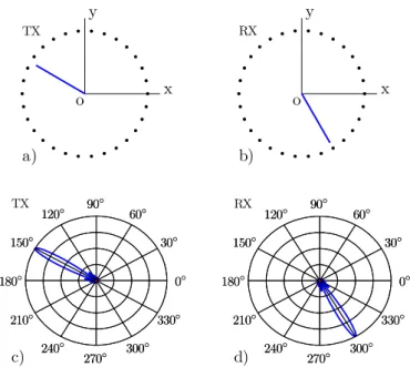
The channel, represented in figures 3a and 3b, consists of 2 paths with different directions and respective amplitudes of 1 and 0.5. Figures 3c and d respectively show the radiation pattern corresponding to each singular value with the transmitter array and the receiver array. The colours correspond to the index of each singular value. There is no, a priori, relation between the colours in the figures a-b and the colours in the figures c-d. The decomposition in singular values allows the identification of 2 nonzero values. When the paths are sufficiently spaced, the number of singular values and the number of propagation paths are identical. The decomposition maintains the relation between direction of departure and direction of arrival of each path. Each singular value carries a particular path and the amplitude of the singular value is approximately proportional to the power of the path.
x y o a) TX x y o b) RX 0◦ 30◦ 60◦ 90◦ 120◦ 150◦ 180◦ 210◦ 240◦ 270◦ 300 ◦ 330◦ 0◦ 30◦ 60◦ 90◦ 120◦ 150◦ 180◦ 210◦ 240◦ 270◦ 300 ◦ 330◦ c) TX 0◦ 30◦ 60◦ 90◦ 120◦ 150◦ 180◦ 210◦ 240◦ 270◦ 300 ◦ 330◦ 0◦ 30◦ 60◦ 90◦ 120◦ 150◦ 180◦ 210◦ 240◦ 270◦ 300 ◦ 330◦ d) RX
Figure 2. Subspace channel with one path configuaration.(a) and (b) represent respectively the arrival ray and the corresponding departure ray. (c)
and (d) represents respectiveley the patterns of the arrival eigenvalue and the corresponding departure eigenvalue.
x y o a) TX x y o b) RX 0◦ 30◦ 60◦ 90◦ 120◦ 150◦ 180◦ 210◦ 240◦ 270◦ 300 ◦ 330◦ 0◦ 30◦ 60◦ 90◦ 120◦ 150◦ 180◦ 210◦ 240◦ 270◦ 300 ◦ 330◦ c) TX 0◦ 30◦ 60◦ 90◦ 120◦ 150◦ 180◦ 210◦ 240◦ 270◦ 300 ◦ 330◦ 0◦ 30◦ 60◦ 90◦ 120◦ 150◦ 180◦ 210◦ 240◦ 270◦ 300 ◦ 330◦ d) RX
Figure 3. Subspace channel with two paths configuration with different amplitudes. (a) and (b) represent respectively the 2 arrival rays and the corresponding 2 departure rays. (c) and (d) represents respectiveley the patterns of the 2 arrival eigenvalues and the corresponding departure
eigenvalues.
This bijection between each singular value and a physical path is not always checked. For a same geometrical configuration, the variation of the amplitude or phase of the path can modify the decomposition significantly. A singular value can be linked to several paths. For example, figure 4 gives results considering the same paths model with identical path amplitudes.
x y o a) TX x y o b) RX 0◦ 30◦ 60◦ 90◦ 120◦ 150◦ 180◦ 210◦ 240◦ 270◦ 300 ◦ 330◦ 0◦ 30◦ 60◦ 90◦ 120◦ 150◦ 180◦ 210◦ 240◦ 270◦ 300 ◦ 330◦ c) TX 0◦ 30◦ 60◦ 90◦ 120◦ 150◦ 180◦ 210◦ 240◦ 270◦ 300 ◦ 330◦ 0◦ 30◦ 60◦ 90◦ 120◦ 150◦ 180◦ 210◦ 240◦ 270◦ 300 ◦ 330◦ d) RX
Figure 4. Subspace channel with two paths configuration with same amplitude. (a) and (b) represent respectively the 2 arrival rays and the corresponding departure rays. (c) and (d) repesents respectiveley the patterns
of the arrival eigenvalues and the corresponding departure eigenvalues.
Each singular value exploits simultaneously the two propagation paths. The subspace radiation patterns beam in 2 directions but not exactly in the real physical direction. The directions of pointing of each singular value present opposite errors. Consequently, the averaged radiation pattern of the singular values is in agreement with the physical paths. This remark is also applicable to the amplitude.
All these results remain valid with an unspecified number of paths but only if the paths are independent. This condition requires having paths sufficiently angularly spaced in comparison to the angular resolution of the array. This condition applies on both sides of the link and to the whole of the paths. If we consider a model with 3 paths of identical amplitudes and with two of them having close directions of arrival. The result illustrated in figure 5, shows that only two eigenvalues are corresponding to the major part of energy.
x y o a) TX x y o b) RX 0◦ 30◦ 60◦ 90◦ 120◦ 150◦ 180◦ 210◦ 240◦ 270◦ 300 ◦ 330◦ 0◦ 30◦ 60◦ 90◦ 120◦ 150◦ 180◦ 210◦ 240◦ 270◦ 300 ◦ 330◦ 0◦ 30◦ 60◦ 90◦ 120◦ 150◦ 180◦ 210◦ 240◦ 270◦ 300 ◦ 330◦ c) TX 0◦ 30◦ 60◦ 90◦ 120◦ 150◦ 180◦ 210◦ 240◦ 270◦ 300 ◦ 330◦ 0◦ 30◦ 60◦ 90◦ 120◦ 150◦ 180◦ 210◦ 240◦ 270◦ 300 ◦ 330◦ 0◦ 30◦ 60◦ 90◦ 120◦ 150◦ 180◦ 210◦ 240◦ 270◦ 300 ◦ 330◦ d) RX
Figure 5. Subspace channel with three paths configuration with same amplitude. (a) and (b) represent respectively the 3 arrival rays and the corresponding 3 departure rays. (c) and (d) repesents respectiveley the patterns of the arrival eigenvalues and the corresponding departure
eigenvalues.
E. 3D Generalization with Polarisation
In order to generalize the previous results, it is essential to consider multipaths in 3D with arbitrary polarization. This study was achieved by replacing each element of the UCA by a ULA of 5 elements. Each element is built of two isotropic antennas in cross polarization. This provides a cylindrical array of 300 antennas with a geometrical shape represented in figure 6. Now, the simulation is taken into account the polarization and the path loss is now expressed by a complex matrix of
dimension2×2 instead of a simple complex value. So the
depolarization of a path can be defined by its matrix.
y zzzzz
x
Figure 6. Cylindrical array.
Let us consider a path having the following geometrical characteristics:
135
departure
θ = ° 45θarrival= ° , 0ϕarrival = °ϕdeparture = ° . 60
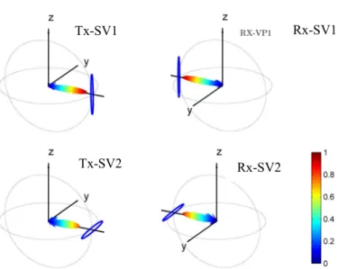
In free space configuration with only one path, the MIMO channel has two singular values with the same amplitude. The number of singular values is doubled. This is due to the independence of two polarizations. The radiation pattern of the singular mode corresponding to each singular value is presented in figure 7. They follow the physical direction of the path. The blue segments, indicating the trajectory of the field
E
G
, show the orthogonality of the polarization between the two subspace radiation patterns.
Figure 7. Subspace radiation patterns with one path.
In the case of depolarization, the number of eigenvalues remains equal two. However, the amplitudes can be very different according to the matrix conditioning of the path. For example, if we consider a channel depolarization of approximately 10%, the module of the power gain is given by
0.9 0.1 0.1 0.9
⎡ ⎤
⎢ ⎥
⎣ ⎦ , and the phase is supposed to be random. The simulation results are represented in figure 8. The singular mode radiation patterns correspond quite well to the physical directions of the paths. However, the energy is no longer the same between the two subspace channels, and the polarization is arbitrary. The first eigenvalue contains most of the energy.
Figure 8. Subspace radiation patterns with one path and depolarization.
Other simulations with different multipaths were also carried out. Even without depolarization, multipaths induce an imbalance of the eigenvalue amplitudes. Apart from the previous remarks, the conclusions obtained in 2D remain valid in 3D.
F. Conclusion
From the development of a propagation channel simulation tool including antenna arrays and the propagation channel, the relation between subspace and physical channels was investigated. All of these simulation results were obtained with circular and cylindrical MIMO arrays. This study shows that the number of eigenvalues corresponds to the number of independent paths. Independence can be defined by an angular spacing higher than the resolution of the antenna array. Apart from some particular cases, there is no “one to one” relationship between the radiation pattern of a singular value and the direction of single path. In fact, a singular value can beam simultaneously in different directions, not corresponding exactly to the physical direction. The number of eigenvalues is doubled when polarization is taken into account. The eigenvalue amplitudes are identical in the case of line-of-sight (LOS) configuration; otherwise they are usually different because of the depolarization induced by the antennas and the channel.
IV. EXPERIMENTAL SUBSPACE CHANNEL IN REALISTIC ENVIRONMENT.
A. Description of the Experimentation
Many experimental studies have been carried out to model the MIMO propagation channel. The most advanced experiments use double directional measurements. However, the complexity is so high that these experiments are simplified and provide only partial information of the channel (3D or polarization is missing for instance). This complexity is further increased in UWB configurations. A good compromise between accuracy and complexity was obtained with an original method presented in [7]. This device is able to study the degree of freedom of the channel thanks to a large number of sensors and the non-ambiguity of the DoA and DoD.
B. Results in anechoic chamber
Experimentation was carried out in an anechoic chamber (figure 9). The distance between the two antenna arrays was 4.5 m. The far-field condition was met from 3 GHz to 10 GHz. Only one path is obtained with this experimental configuration. The degree of freedom is defined as the number of highest singular values whose sum is equivalent to 90% of the total power. Only two degrees of freedom were obtained by analyzing the results, whatever the frequency. This result is in agreement with the simulation results. Figure 10 shows that the directions of the subspace channel are in agreement with the position of the antennas. However, the amplitudes are not perfectly identical, and polarizations are not perfectly orthogonal. This is probably due to antenna depolarization.
Tx-SV1 Rx-SV1
Tx-SV2 Rx-SV2
Tx-SV1 Rx-SV1
Figure 9. Anechoic chamber environment
Figure 10. Subspace radiation patterns in the anechoic chamber.
C. Evaluation in a actual environment
Experimentation was performed in a meeting room in order to investigate the number of degrees of freedom in actual configuration. A 360° panoramic picture, shot from the emitter location and presented in figure 11, shows the environment. Contrary to the anechoic chamber, this LOS configuration shows multipaths. The number of degree of freedom is larger. Moreover, the number of degrees of freedom increases with the frequency contrary to their behavior in the anechoic chamber. This is due to the improvement of the MIMO array resolution when the frequency increases. This characteristic allows the identification of additional paths and thus increases degrees of freedom. An analysis shows an increase in the number of eigenvalues with the delays. This is explained by the increase of propagation phenomena when the delay increases. At the opposite, the direct path has only 2 eigenvalues.
V. CONCLUSION
MIMO channel simulations using circular and cylindrical arrays highlighted the relations between physical and subspace channels. The number of singular values of the transmission channel corresponds to the number of independent paths. The independence of the paths depends on the angular resolution of the MIMO array and on the DoA and the DoD of the paths. There is no bijective relation between the subspace channels
and the multipaths. This investigation was also carried out by experimentation. An original MIMO UWB device was used in an anechoic chamber and in a real environment. An analysis concerning the evolution of the eigenvalues according to the frequency and the environment was completed..Future study will investigate other representative environments, such as residential environment.
Figure 11. Meeting room environment
Figure 12. Degrees of freedom analysis in meeting room configuration VI. REFERENCES
[1] E. Bonek, M. Herdin, W. Weichselberger, and H. Özcelik, "MIMO - Study Propagation First," presented at IEEE International Symposium on Signal Processing and Processing and Information Technology, Darmstadt, 2003.
[2] N.Malhouroux-Gaffet, P. Pajusco, E. Haddad"Effect of propagation phenomena on MIMO capacity of wireless systems between 3 and 10 GHz " EUCAP 2010, Barcelona, Spain2010
[3] C.E. Shannon, A Mathematical Theory of Communication, Bell System
Technical Journal, vol. 27, p. 379-423 and 623-656, July and October,
1945.
[4] S. Loyka, "Multiantenna capacities of waveguide and cavity channels,"
Canadian Conference on Electrical and Computer Engineering, 2003. IEEE CCECE 2003. 4-7 May 2003, vol. vol.3, pp. 1509- 1514, 2003.
[5] M. Steinbauer, A. F. Molisch, and E. Bonek, "The double-directional radio channel," Antennas and Propagation Magazine, IEEE, vol. 43, pp. 51, 2001.
[6] J. M. Conrat and P. Pajusco, "A Versatile Propagation Channel Simulator for MIMO Link Level Simulation," EURASIP Journal on
Wireless Communications and Networking, 2007.
[7] P. Pajusco, G. Tesserault, N. Malhouroux, and C. Sabatier, "Novel array structure for space-time characterization of the UWB channel", PIMRC 2008. IEEE 19th International Symposium on, 2008.
3 4 5 6 7 8 9 10 8 10 12 14 16 18 20 22 24 D egrees of free dom Frequency [GHz] Tx-SV1 Rx-SV1 Tx-SV2 Rx-SV2