Distributed control of electromechanical oscillations in very large-scale electric power systems

(1)

UNIVERSITY OF LIEGE

DEPARTMENT OF ELECTRICAL ENGINEERING

AND COMPUTER SCIENCE

DISTRIBUTED CONTROL OF

ELECTROMECHANICAL OSCILLATIONS

IN VERY LARGE SCALE ELECTRIC

POWER SYSTEMS

BY

DA WANG

SUBMITTED IN PARTIAL FULFILLMENT OF THE

REQUIREMENT FOR THE DEGREE OF DOCTOR

OF PHILOSOPHY IN ENGINEERING SCIENCE

DOCTORAL THESIS

(2)

(3)

Abstract

Electromechanical oscillations were observed in power systems as soon as synchronous generators were interconnected to provide more power capac-ity and supply reliabilcapac-ity. These oscillations are manifested in the relative motions of generator mechanical axes accompanied by power and voltage oscillations. Some characteristics of modern large-scale electric power sys-tems, such as long transmission distances over weak grids, highly variable generation patterns and heavy loading, tend to increase the probability of appearance of sustained wide-area electromechanical oscillations. The term “wide-area” is used here to emphasize the possible co-existence of local and inter-area oscillation modes of different frequencies that might appear simul-taneously in different parts of large-scale systems. Such oscillations threaten the secure operation of power systems and if not controlled efficiently can lead to generator outages, line tripping and even large-scale blackouts.

In general, it is usually considered that electromechanical oscillations are caused by insufficient system damping. Due to the limited reinforcement available for current network structure, most of efforts for electromechanical oscillations damping focus on setting different controllers such as Power Sys-tem Stabilizers (PSSs), Thyristor Controlled Series Compensators (TCSCs), and so on, in order to improve system damping. These damping controllers mostly use local measurements at their inputs, and their control rules and parameters are determined in off-line studies using time-domain simulations, Prony or eigenanalysis, and usually remain fixed in practice.

However, increasing uncertainties brought by renewable generation, and the growing complexity resulting from new power flow control devices, could make the damping effects of these designs become questionable in practice. Moreover, the controllers scattered into different areas and installed at differ-ent momdiffer-ents are to be further coordinated to obtain better global damping performances. So, it yields the need for more efficient, adaptive, and more

(4)

widely coordinated damping control schemes.

To this end, this thesis proposes a trajectory-based supplementary damp-ing control. It treats dampdamp-ing control as a multi-step optimization control problem with discrete dynamics and costs, which calculates supplementary input signals for existing controllers using model-based methods or learning-based methods. At each control time, it collects current system states, solves the optimal control problem and superimposes the calculated supplementary inputs on the outputs of existing controllers. With the help of these supple-mentary inputs, it forces the controlled system response to evolve along the desired trajectory. These supplementary signals are continuously updated, which allows to adaptively adjust and coordinate a subset of the existing damping controllers, and eventually all of them.

Assuming that power system dynamics can be quite accurately modeled, and given the recent progresses in large-scale optimization, a natural idea is to apply Model Predictive Control (MPC) to embody the proposed control scheme. MPC is a proven technique with numerous real-life applications in different engineering fields and it may be designed in different ways: central-ized, distributed and hierarchical.

In this thesis, firstly, a fully centralized MPC scheme is designed based on a linearized, discrete, complete state space model. Its performances are evaluated both in ideal conditions and considering realistic state estimation errors, and computation and communication delays. The effects of the num-ber and type of available damping controllers are also studied in order to assess the versatility of this scheme. This scheme is further extended into a distributed scheme with the aim of making it more viable for very large-scale or multi-area systems. Different ways of decoupling and coordinating between subsystems are analyzed. Finally, a robust hierarchical multi-area MPC scheme is proposed, introducing a second layer of MPC based con-trollers at the level of individual power plants and transmission lines. The performances of these three MPC schemes are illustrated and compared on a 16 generators, 70 buses test system.

While MPC, being a closed-loop control scheme, has some intrinsic level of robustness to modeling errors, it nevertheless relies on the use of a correct dynamic model of the system. Within the context of power system oscil-lation damping, load-dynamics, and dynamics of renewable and dispersed generation may have a significant impact on the system behaviour; since the composition of the load and dispersed generation may change significantly from one period of time to another (e.g. intra-daily, and seasonal effects

(5)

iii driven by weather conditions) the system dynamics at a particular moment may not be well enough approximated by the model computed from the avail-able data in TSO control centers to yield satisfactory performances of any one of the proposed MPC schemes.

Another supplementary damping control, considered in this thesis, is based on model-free learning methods. Specifically, a tree-based batch mode Reinforcement Learning (RL) algorithm is applied in place of MPC to cal-culate the supplementary signals for existing damping controllers. Using a set of dynamic and reward four-tuples, it constructs an approximation of the optimal Q-function over a given temporal horizon by iteratively extending its prediction horizon. In each iteration, the Q-function is approximated by an ensemble of extra-trees. Between two iterations, the Q-function is refreshed using the obtained instantaneous rewards at current step and the Q-function of the previous step. The actions greediest with respect to the Q-function are applied as supplementary signals to existing damping controllers. The scheme is firstly tested on a single generator, and then on multiple generators. Finally, the combined control effects of MPC and RL are also investigated.

(6)

(7)

Acknowledgments

First of all, I would like to express my sincere gratitude to my professor, Louis Wehenkel, for the valuable research opportunity and guidance given by him. I really learned a lot from his thorough insight into power systems stability and control, and his way of carrying out research.

I most deeply thank Mevludin Glavic for his very useful advices and constant help in my research.

I acknowledge the funding of University of Li`ege, which has supported

my research and life during the past four years. This thesis presents research results of the Belgian Network DYSCO, funded by the Interuniversity Attrac-tion Poles Programme, initiated by the Belgian State and of the PASCAL Network of Excellence funded by the European Commission. The scientific responsibility rests with the author.

I thank the members of the Jury for devoting themselves to read this manuscript and to all the related duties.

I am also indebted to Samuel Hiard for his help in my study and life, to Raphael Fonteneau for helping out with the fitted Q iteration code, to Diane Zander, and other colleagues and friends of Montefiore Institute.

(8)

(9)

List of acronyms and symbols

Acronyms

AC Alternative Current DAE Differential Algebraic

Equa-tion

DC Direct Current DP Dynamic Programming

EMS Energy Management

Sys-tem

EW East West oscillation mode

FACT Flexible Alternative Cur-rent Transmission

HVDC High Voltage Direct Cur-rent transmission

LC Local Controller MC Monte Carlo

MPC Model Predictive Control PSS Power System Stabilizer

PST Power System Toolbox RL Reinforcement Learning

QP Quadratic Programming RAM Random Access Memory

SE State Estimation SSSC Static Synchronous Series

Compensator

STAT-COM

Static Synchronous Com-pensator

SVC Static Var Compensator

TCSC Thyristor Controlled Series Compensator

TD Temporal Difference

TG Turbine Governor TSO Transmission System

Oper-ator UCTE Union for the Coordination

of the Transmission of Elec-tricity

ULC Unstable limit Cycle

UPFC Unified Power Flow Con-troller

WAMS Wide Area Measurement

System vii

(10)

Symbols

A State matrix Aˆ Supervised learning

algo-rithm ˆ

a Attribute B Input matrix

C Output matrix cˆ Lower MPC correction

d Variable number dˆ Output feedback

ˆ

E Expectation E˜_d0 d axis component of stator

voltage ˜

Ef Field voltage E˜q0 q axis component of stator

voltage ˜

Er Electromotive force at the

receiving end

˜

Es Electromotive force at the

sending end

f Input-output function Gˆ Transfer function

ˆ

H Hypothesis space of

input-output function

˜

Is Current at the sending end

i Discrete dynamic step ˆi State-action pair input

j Iteration number ˆj ˆj-th test

ˆ

K Attribute number k MPC control time step

ˆ

k k-th attributeˆ L Expected loss over a

learn-ing sample set

l l-th row in a matrix or

ele-ment of a vector

ˆ

l Loss function

M Tree number Mˆ Sample number

m m-th subsystem mˆ m-th sampleˆ

N Local controller number n n-th local controller

ˆ

nmin Leaf node size oˆ Output of state-action pair

P Power Pˆ Probability distribution

p Differential operator pˆ p-th evolution pathˆ

Q State-action value function R Control return over a time

horizon ˆ

R Line resistance R˜f Exciter state

r One-step instantaneous

re-ward

S RL state space

ˆ

S Score for a splitting S˜s Complex power at the

(11)

ix

s[t] Set-point trajectory s RL state

U Control action space u, ˆu Control action and

esti-mated value

T Matrix transposition Tˆ Tree

Th Prediction horizon Tc Control horizon

t Time ˆt Test threshold value

V MPC cost function V˜l Load bus voltage

Vr Regulator voltage Vref Voltage reference of exciter

Vt Generator terminal voltage Vpss PSS output

W Weight matrix X Power system state space

ˆ

X Line reactance x, ˆx Power system state and

es-timated value

Y Measured output space y, ˆy Measured output and

esti-mated value

yref Output reference Z Controlled output space

˜

Zl Load impedance Z˜r Line impedance at the

re-ceiving end ˜

Zsr Mutual-impedance Z˜ss Self-impedance

˜

Zs Line impedance at the

send-ing end

z, ˆz Controlled output and

esti-mated value

α Searching step of Active Set

methods

ˆ

α Time Difference learning

variable

γ Discount factor ∆ Increment

δ Rotor angle δˆ Time dynamic

ε A small probability value θ Rotor angle difference

π Control policy τ Delay

˜

ψ_d00 d axis air gap flux linkage ψ˜_q00 q axis air gap flux linkage

˜

ψ1d Amortisseur circuit flux

linkages of d axis

˜

ψ1q Amortisseur circuit flux

linkages of q axis

ω Generator speed ωref Generator speed reference

R Real number space T S Training set

(12)

(13)

Part I

Introduction

(20)

(21)

Chapter 1 Power system

electromechanical oscillations

1.1 Oscillation modes

Electromechanical oscillations in power systems are usually characterized by low frequency and poor damping. The stability of these oscillations is of vital concern, and is a prerequisite for secure system operation.

In terms of oscillation ranges and frequencies, electromechanical oscilla-tions can be divided into two categories [1, 3]:

• Local modes: oscillations associated with a single generator or a single power plant. These oscillations have the frequencies in the range 0.7 to 2Hz. In some cases, local oscillations can excite other oscillation modes, namely inter-area modes.

• Inter-area modes: the generators in one sub-area oscillate against the generators in other sub-areas. Inter-area oscillations have their fre-quencies in the range 0.1 to 0.8Hz. Once excited, inter-area oscillations may propagate over the whole system.

As far as this thesis is concerned, the focus is on inter-area electromechan-ical oscillations analysis and control. Let us take the European power system as an example to illustrate electromechanical oscillations [4]. The intercon-nected synchronous power system of continental Europe (former UCTE) ex-tends from Greece and Iberic peninsula in the south, to Denmark and Poland

(22)

Figure 1.1: European interconnection synchronous areas. Taken from [4] to the north and up to the border of the Black Sea to the east, as shown in Fig. 1.1. It is the largest interconnected system in the world, and in the year 2012 [5] it supplied power to about 500 million customers in 24 countries with a total annual energy consumption of approximate 3336TWh. In the same year this system had a peak load of about 508GW [5]. The system is operated in a decentralized way, by a group of about 40 TSOs, each one being responsible for a given control zone, assisted by two coordination centers.

In a classical scenario with a power flow of 350MW from Spain to France and of 1300 MW from CENTREL (Poland, Czech Republic, Slovakia and Hungary) to UCTE, four dominant inter-area modes (also called global modes) are identified in the low frequency range 0.2 to 0.5 Hz (adapted from [6]):

• Global mode 1: the generators in Spain and Portugal swing against the generators in the eastern part at a frequency of 0.2Hz.

• Global mode 2: this mode has a frequency of about 0.3 Hz and forms three coherent groups of generators. The generators in Spain and Por-tugal (group1) are almost in phase with the generators of CENTREL and eastern parts of Germany and Austria (group 2). The third group

(23)

1.2. MATHEMATICAL FORMULATIONS 5 (France, Italy, Switzerland and western parts of Germany and Austria) is in phase opposite to the other two groups.

• Global mode 3: it appears at a frequency of about 0.5 Hz and involves mainly the generators in Poland and Hungary. The parts of Austria, Slovakia and Italy are also involved while the rest UCTE system is almost not involved.

• Global mode 4: it is observed close to 0.5 Hz. This mode does not seem to be critical for the East-West transit (between UCTE and CEN-TREL) but has to be observed carefully in case of bulk power transfers from the North to the South.

Among these four oscillation modes, global mode 1 and 2 are the most interesting as they involve almost the whole interconnected system. Due to the foreseen interconnection of Turkey to the UCTE interconnected system, a new inter-area mode, close to 0.15 Hz, will probably appear [7].

Similar electromechanical oscillations are also detected in other intercon-nections around the world [8, 9].

Oscillations are acceptable as long as they decay rapidly enough. Sus-tained and increasing oscillations can cause generator outage, line tripping, network splitting and even blackout. Usually, the restriction or even the curtailment of power exchange among interconnected areas is the most effec-tive operational measure avoiding such undamped oscillations. However, it is not the most effective approach from the economical point of view. More economical damping controls are discussed at the end of this chapter.

1.2 Mathematical formulations

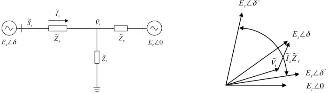
Mathematical insights into electromechanical oscillations can be obtained with the help of a two-generator system shown in Fig. 1.2. The amplitudes of electromotive force ˜Es and ˜Er are assumed to be constant. ˜Er is taken as

the reference and the shunt capacitances of transmission line are ignored. ˜Zs

and ˜Zr are the transmission line impedances at the sending end and at the

receiving end. ˜Zl represents a constant impedance load. Based on the circuit

(24)

s S~ δ ∠ s E r Er∠0 Z~ l Z~ ! Vl s I ~ s Z~ 0 ∠ r E δ ∠ s E δʹ′ ∠ s E δʹ′ʹ′ ∠ s E ! V_l IsZs ~ ~

Figure 1.2: Two-generator system and corresponding phasor diagram

˜ Is= ˜ Es ˜ Zss − E˜r ˜ Zsr = ˜ ZlEr ˜ ZsZ˜l+ ˜ZsZ˜r+ ˜ZrZ˜l [Es Er ( ˜ Zr ˜ Zl + 1)ejδ − 1] (1.1)

where ˜Zss is the self-impedance and ˜Zsr is the mutual-impedance.

˜ Zss = ˜Zs+ ˜ ZrZ˜l ˜ Zl+ ˜Zr ; Z˜sr = ˜Zs+ ˜Zr+ ˜ ZsZ˜r ˜ Zl ; (1.2)

The complex power at the sending end is:

˜ Ss= ˜EsI˜s∗ = ˜ ZlEsEr ˜ ZsZ˜l+ ˜ZsZ˜r+ ˜ZrZ˜l [Es Er ( ˜ Zr ˜ Zl + 1) − ejδ] (1.3)

And the voltage at the node l is:

˜ Vl = ˜Es− ˜IsZ˜s = ˜ ZsZ˜rEr ˜ ZsZ˜l+ ˜ZsZ˜r+ ˜ZrZ˜l ( ˜ ZlEs ˜ ZsEr ejδ+ 1) (1.4)

The equations (1.1), (1.3) and (1.4) show when δ fluctuates in a certain range, the electrical variables like line current, transmission power and node voltage all will fluctuate correspondingly following δ. The right part of Fig.1.2 is an example of voltage fluctuation when δ varies from δ0 to δ00.

(25)

1.3. ELECTROMECHANICAL OSCILLATION MECHANISMS 7

1.3 Electromechanical oscillation mechanisms

1.3.1 Negative damping

It is usually considered that electromechanical oscillations are caused by in-sufficient damping or negative damping in power systems. The damping of power systems normally depends on system structures, controller parameters and operation conditions:

• System structures: electromechanical oscillations occur when existing generation/load areas are connected to other similar areas by relatively weak transmission lines. Weak connection means large inter-area line

impedances. The frequencies and damping ratios1 _{of inter-area}

oscil-lations drop as the inter-area line impedances increase. The inter-area DC links, parallel to AC tie-lines, can strengthen the inter-area con-nection and do not introduce new inter-area oscillation modes. But the DC links can affect the frequencies and damping ratios of existing inter-area modes [3]. In addition, when the high impedance lines are parallel with the low impedance lines, the loss of low impedance lines may cause instable inter-area oscillations [11].

• Controller parameters: an exciter is of major help in providing the synchronizing torque, but it also may destroy the natural damping of power systems [12]. The effect of a single fast exciter on damping depends on its location in the system, and the types of exciters on other generators [3]. Power System Stabilizer (PSS) is the most cost-effective method of enhancing the damping of electromechanical oscil-lations. But when a local power system is incorporated into a large power system, PSS parameters in this area must be verified carefully and adjusted in order to achieve a positive contribution for damping inter-area oscillations [6].

• Operating conditions: the damping of inter-area oscillations is also in-fluenced by power flows. For example, the next foreseen expansion of European power system is the interconnection of Turkey power system to UCTE. The analysis of paper [7] shows that when Turkey exports

1_{For a pair of complex eigenvalues λ = σ ± jω, the damping ratio ζ is ζ = −}_√ σ σ2_+ω2.

(26)

active power, the damping of inter-area mode EW-1 is strongly de-creased.

• Load characteristics: electromechanical oscillations are accompanied by voltage oscillations at load nodes, and hence cause load variations. Conversely, load variations will influence system voltage profiles and influence electromechanical oscillations. So, it forms a feedback loop between loads and electromechanical oscillations. Load characteristics, including constant impedance, constant current, constant power char-acteristics and the rate of load recovery, all affect load response to voltage variations. It may alleviate or aggravate power system elec-tromechanical oscillations [13, 14].

1.3.2 Other causes

In addition to the above described negative damping mechanisms, there are other causes of electromechanical oscillations:

• Forced oscillations: for power systems containing the sources of forced oscillations, such as various types of cyclic loads, diesel engine driven generators and wind turbine driven generators, if the frequency of any of electromechanical oscillation modes coincides with that of forced oscillations, a resonance phenomenon will occur. When the inherent damping of electromechanical oscillations is lower, the resonance of forced oscillations with an electromechanical oscillation mode could lead to a complete system breakdown [15].

• Modal (strong or weak) resonance: it appears when eigenvalue pairs of two stable oscillatory modes coincide approximately, due to the changes in power system operating parameters: the two pairs of eigenvalues first approach one another, interact, and then one of the eigenvalue pairs may cross the imaginary axis and become unstable [16, 17].

• Bifurcations: when the state matrix A has a pair of purely imaginary eigenvalues (a mode with zero damping), a Hopf bifurcation is said to occur. By carrying out certain Taylor series nonlinear computations, the mode can be classified to be supercritical (nonlinear stable), or subcritical (nonlinear unstable). For the subcritical Hopf mode, there exist unstable limit cycles (ULC) which bound the region of attraction

(27)

1.4. ANALYSIS METHODS 9 around small signal stable equilibria. The ULC defines the bound-ary separating oscillations of decreasing amplitude (positive damping response) and oscillations of growing amplitude (negative damping re-sponse). So, the oscillation stability can be judged by checking whether the post-fault initial condition is inside or outside the transient stability boundary anchored by a ULC [18, 19].

1.4 Analysis methods

1.4.1 Linear methods (adapted from [1])

The distinguishing feature of linear methods is to linearize a nonlinear power system at an equilibrium to obtain a linearized state space model. Based on a linearized model, modal analysis is used to calculate the eigenvalues of state matrix A. The eigenvalues may be real or complex. Since the state matrix A is real, the complex eigenvalues occur in complex conjugate pairs. Each complex conjugate pair of eigenvalues corresponds to one oscillation mode. By modal analysis, the dynamic behaviors of power systems under all different oscillation modes can be investigated and all unstable or weakly damped oscillation modes can be detected. The participation factor indicates the influence of one state to a mode, which gives very useful information on the most efficient location to undertake any possible control measure.

Modal analysis describes the small signal behaviors around a specific op-erating point. The nonlinear behaviors during large perturbations are not taken into account. So, the damping controls designed using modal analysis must be tested by nonlinear simulations under a wide range of operating conditions and faults, in order to assure their control effects in practice [1].

1.4.2 Nonlinear methods

All nonlinear methods involve Differential Algebraic Equations (DAE) that depict system dynamics. Time domain simulation is the most prevalent non-linear method and it is widely used by power system operators and planners to study power system dynamics. It firstly builds a system-wide model by combining all devices’ DAE according to power system topology. Then, tak-ing a certain operattak-ing point as the initial value, it calculates state variables and algebraic variables step by step with the help of different mathematical

(28)

techniques. If the simulation is continued for a sufficiently long time, it is possible to determine whether electromechanical oscillations decay with time (they are stable), or continue at a constant amplitude or increase in ampli-tude (they are unstable) by observing rotor angle trajectories, tie-line power trajectories or other state trajectories. The advantage of time domain simu-lation is to all the modeling of all nonlinear and discrete dynamics. But in practice, the time required for time domain simulation is long and the com-putation is large. Moreover, it only can tell whether the post-disturbance system is stable or not for a given set of scenarios, but it can not provide a deeper insight about oscillation modes [1].

Except for solving DAE step by step, we also can perform a two-order Tay-lor series expansion of DAE in the neighborhood of an operating point, and further transfer Taylor series into normal form or modal series to calculate system response including the nonlinearity. Contribution factor, nonlinear participation factor and other nonlinear indices derived from the higher-order items can provide more refined information about nonlinear interaction be-tween the fundamental oscillation modes, which is unavailable in linear modal analysis [20, 21].

1.4.3 Signal analysis methods

Signal analysis methods, like Wavelet transform, Prony analysis and Hillbert-Huang transform [22–24], can directly extract electromechanical oscillation mode information from response curves obtained from measurements gotten from practical operation or from time-domain simulations.

Among these methods, the one most used is Prony analysis.

Defining the output as a linear combination of exponential functions, the basic Prony analysis estimates the damping, phases and magnitudes of electromechanical oscillation modes by solving a least-squares problem using evenly sampled data [25]. But, the estimation precision of Prony analysis may deteriorate due to the existence of measurement or simulation inaccura-cies (e.g. noise, or inappropriate sampling frequeninaccura-cies). Multi-signal Prony analysis, input signal pre-filtering and iterative Prony method all can improve the precision of Prony analysis [26–28].

In addition, in the condition assuming the input is a finite summation of delayed signals with the same characteristic eigenvalue, Prony analysis can identify a reduced-order transfer function incorporating local and inter-area electromechanical oscillatory modes [23].

(29)

1.5. CONTROLLERS AND ACTUATORS 11

1.5 Controllers and actuators

Strengthening grid structure can improve power system damping and elec-tromechanical oscillation stability. However, it is uneconomic and difficult to be realized due to economic and environmental constraints. On the other hand, diverse controllers and actuators are placed in power systems initially for certain reasons other than to damp oscillations. Once installed, these de-vices also can be used to increase the damping of certain electromechanical oscillation modes [1, 10].

1.5.1 PSS

PSS is the most cost-effective electromechanical oscillation control. It uses auxiliary stabilizing signals, like generator shaft speed and accelerating power to produce an additional component of electrical torque proportional to speed change for its excitation to increase electromechanical oscillation damping. During the past three decades, extensive researches were paid to PSS place-ment and parameter setting, which made PSS become a technologically ma-ture and widely used damping control.

1.5.2 FACTs devices

FACTs do not indicate a particular controller but a host of controllers like Static Var Compensator (SVC), Static Synchronous Compensator (STAT-COM), Thyristor Controlled Series Compensator (TCSC), Static Synchronous Series Compensator (SSSC), and Unified Power Flow Controller (UPFC). FACTs devices can flexibly and rapidly control node voltages, change line impedances and adjust power flow to enhance the damping of electrome-chanical oscillations.

1.5.3 HVDC modulation

Using HVDC modulation to damp AC system oscillations is another inter-esting technique. The damping of electromechanical oscillations in an AC system can indeed be increased by modulating the current at the rectifier or the current and voltage at the inverter. The design of the modulation scheme must however be tailored to a specific system [29].

(30)

While all the previous methods provide a set of potentially effective tools to help damping electromechanical oscillations, their controller tuning needed to reach an optimal level of damping may be sensitive to prevailing system op-eration conditions (such as topology, genop-eration pattern, and loading level).

1.6 Conclusions

In this chapter, electromechanical oscillations have been shortly described, and some examples of oscillations in the UCTE power system were given. Furthermore, the evolution of electrical states in oscillations was illustrated mathematically using a two-generator equivalent system. Several factors, which influence power system damping, have been discussed. Electrome-chanical oscillations could be studied using linear methods, nonlinear meth-ods and signal analysis methmeth-ods.

Three types of frequently used oscillation damping controls have been briefly discussed. In practice, diverse damping controllers nonlinearly in-teract and jointly decide control effects. Introduction of new damping con-trollers could jeopardize damping effects of existing concon-trollers [6]. Conse-quently, it is very important to coordinate diverse damping controllers and adjust their parameters following the evolution of operation conditions, in order to obtain satisfactory and robust control effects. It is the objective that this thesis attempts to achieve.

(31)

Chapter 2 Research motivations, methods

and contributions

2.1 Research motivations

Electromechanical oscillations, especially inter-area electromechanical oscil-lations, become more common in large-scale interconnected power systems. Fig. 2.1 gives an example of inter-area electromechanical oscillations in the

European power system [30]. These oscillations restrict inter-area power

exchange, propagate disturbances over the whole system and even lead to blackouts, if cascading outages are caused [31–33]. Different controllers, like PSSs, TCSCs and SVCs, are already designed for damping electromechanical oscillations.

The typical model-based design of damping controllers of electromechan-ical oscillations normally begins with the recognition of oscillation modes, then proceeds to determine controller parameters producing better damping performances and robustness, and ends with the verification via time-domain simulations [1, 34]. The control rules and parameters are usually calculated based on local information and objectives, and remain “frozen” in practi-cal application. In recent researches on electromechanipracti-cal oscillations, some remote information reflecting global dynamics is introduced as additional inputs to local damping controllers so as to enhance their performances of damping inter-area oscillations [35–37].

However, increasing uncertainties brought by the renewable generation, and the growing complexity resulting from new power flow control devices,

(32)

Fig. 2 Inter-Area Oscillation after Power Plant

Outage in Spain, 900MW

Fig. 4 Simulation of Power Plant Outage in

Spain, 900 MW

Fig. 3 Inter-Area Oscillation after Load Outage in Spain, 487 MW

Fig. 5 Simulation of Load Outage in Spain, 500MW

signals, that equip a significant number of genera-tion units with a great positive influence on damp-ing of inter-area oscillations.

In the analysis the controllers of CENTREL were at first considered with their origin settings before activities for optimising were undertaken. The effect of parameter optimising on system behaviour is taken into account in chapter 5.

3.2 Model Validation

The model could be validated by the recordings collected from WAMS. As an example Fig. 4 and Fig. 5 show the simulation results after power plant outage and load outage in Spain respectively, which have to be compared with the recordings in Fig. 2 and Fig. 3. It can be concluded that the model represents the real system behaviour with sufficient accuracy regarding the analysis of inter-area oscillations. The dynamic characteristics of power flows and frequencies at different locations are in well accordance with the recordings,

16.12.97; 16:19:... 49,92 49,93 49,94 49,95 49,96 49,97 35,5 55,5 15,5 35,5 55,5 15,5 35,5 55,5 15,5 35,5 55,5 time f [Hz] -900 -850 -800 -750 -700 -650 -600 P [MW] f ≈ 0.22 Hz

active power: Vigy (France) - Uchtelfangen (Germany) (one 400-kV-system)

frequency: Cantegrit (France, near Spain) frequency: Uchtelfangen (Germany, near France)

Spain

Poland

Germany (border to France)

active power France-Germany (one 400-kV system 0 3 6 9 12 15 seconds 15 5 -5 -15 -25 -35 -45 -55 -65 -75 -∆∆∆∆f [mHz] -20 -10 0 10 20 30 0 10 20 30 40 seconds ∆∆∆∆f [mHz] -100 -50 0 50 100 150 200 ∆∆∆∆P [MW]

France (Border to Spain) Germany (Border to France)

frequency

active power Germany - France

49,93 49,94 49,95 49,96 49,97 49,98 49,99 50,00 50,01 50,02 33 35 37 39 41 43 45 47 time f [Hz] -600 -500 -400 -300 -200 -100 0 P [MW] Spain France

Germany (border to France)

Germany (east) Hungary Poland f = 0 26 Hz 17.01.97;01:38:... active power:

Vigy (France) - Uchtelfangen (Germany) (one 400-kV-system)

frequencies

Figure 2.1: Inter-area oscillations after power plant outage in Spain. Taken from [30]

make the robustness of this typical design approach become questionable. Moreover, the controllers scattered into different areas and installed at dif-ferent moments need to be further coordinated so as to obtain satisfactory global performances. Improper combination of diverse controllers could in-deed potentially deteriorate the damping level of electromechanical oscilla-tions [6].

This thesis investigates methods to adjust and coordinate existing damp-ing controllers to improve further their global dampdamp-ing effects. This work is done from the following perspectives:

• Global information: due to the continuous extension of interconnected power systems, damping controllers designed based only on local in-formation cannot always efficiently damp inter-area electromechanical oscillations. In order to obtain better global damping effects, a con-troller can benefit from a wider view of the system. That is to say, it should know more about the interaction between its dynamics and controls with external dynamics and controls when it makes a control decision.

Emergence of new technological solutions such as synchronized phasor measurements and improved communication infrastructure enable the development of Wide Area Measurement Systems (WAMS) [38] and

(33)

2.1. RESEARCH MOTIVATIONS 15 the design of new types of controllers [39]. These controllers may be designed from the perspective of the whole system, focus on a wider spectrum of oscillation modes and offer improvements with respect to current local control strategies.

• Optimization: most damping control schemes only target to meet the minimum stability criterion, for example defined by a damping ratio larger than 0.05. Little work is dedicated to optimize damping control effects [40]. A scheme considering damping control optimization might potentially bring better control effects.

• Adaptivity: modern power systems abound with uncertainties on gen-eration schedules, load patterns, and network topologies [41]. The real damping characteristics of power systems are complicated and volatile. A good damping scheme should be able to automatically adjust its control policies following such changes in the power system [42]. • Coordination: global damping effects are decided by all controllers

ex-isting in the system, which makes it important to coordinate their control efforts [43, 44]. A good damping control scheme should be able to make full use of available controllers and avoid the counteraction of damping effects.

The ultimate goal of all efforts to design, coordinate, and adapt damp-ing controllers is to make the controlled system dynamics better meet the requirement of damping electromechanical oscillations.

In this thesis, a trajectory-based supplementary damping control is de-signed, which is superimposed on existing damping controllers (PSSs, TCSCs, and so on) to achieve the above improvements. It treats damping control as a discrete-time, multi-step optimal control problem. At a sequence of mea-surement times, it collects current system meamea-surements, and based on these latter, it determines supplementary inputs to be applied at the next control time to existing damping controllers in order to obtain the maximum control return over a given temporal horizon. The objective of damping electrome-chanical oscillations can be achieved by defining a particular control return. For example, one can define the control return of a sequence of supplemen-tary damping inputs as the negative distance between angular speeds and the rated angular speed over a future temporal horizon. Maximizing the return will force angular speeds to return and remain near the rated speed, and

(34)

when all generators run at this speed, oscillations are damped. Thus, opti-mization of these supplementary inputs brings adaption and/or coordination to the existing damping controllers without the need for changing their own structures and parameters. The above optimization is carried on repeatedly and supplementary inputs are updated adaptively at a series of subsequent times by taking into account changes in the power flows and topology of the power system.

2.2 Trajectory-based supplementary control

In this chapter, the proposed trajectory-based supplementary damping con-trol is introduced in terms of feasibility, overall principle, mathematical for-mulation of the control objective, solution approaches and implementation strategy.

2.2.1 Feasibility

The feasibility of the proposed method derives from the following advances in power systems’ technology, machine learning, and large-scale optimization.

• Dynamic and real-time measurements: WAMS can provide real-time and synchronized information about system dynamics, especially the information closely related to the recognition of oscillation modes and the improvement of global damping performances [45–48];

• Future response prediction: if a system model is available, future re-sponse of power systems can be approximately modeled; if not, the return over an appropriate temporal horizon of one damping control can be learned from the observation of power system trajectories in similar conditions, and then used to approximately predict the effect of controls on the future system response;

• Efficient algorithms: model-based methods and learning-based meth-ods [49–51] have evolved a lot in the last twenty years by exploiting ongoing progress in terms of optimization and machine learning algo-rithms.

(35)

2.2. TRAJECTORY-BASED SUPPLEMENTARY CONTROL 17 t0 t1 t2 t3 time ref x0 u10 u31 u12 u22 u32 u21 u₁₁ u₂₀ u30

Figure 2.2: Trajectory-based supplementary damping control

2.2.2 Overall principle of the proposed method

The power system is considered in this work as a discrete-time system (power system dynamics are continuous in essence, but in our framework we consider discrete-time dynamics). Its trajectories are considered as time evolution of state variables of the controlled system. If the system model is available in the form:

xt+1 = f (xt, ut), (2.1)

then it is possible to compute all future system dynamics by iterating Eqn. (2.1), and based on them optimize control policies. In Eqn. (2.1), xt is a state

vec-tor consisting of elements of the state space X, and ut is an input vector

whose items are elements of action space U (random disturbances can be considered as a subset of these inputs).

If the system model is not available, then its trajectories can still be recorded by using a real-time measurement system.

In both cases constraints on states and actions can in principle also be incorporated by restricting the set of possible states and by restricting the actions that are possible for individual states.

Using certain supplementary inputs, we can force system dynamics to evolve approximately along the desired trajectories in which oscillations are damped, while taking into account random disturbances, prediction inac-curacy, measurement errors, and so on. This is the underlying concept of trajectory-based damping control.

This idea is illustrated in Fig. 2.2, which describes three possible angular

speed trajectories of one generator. From an initial state x0, the angular

(36)

1, 2, 3. The target is to search a particular sequence of discrete supplementary inputs to the damping controller on this generator (exciter or PSS), in order to drive its angular speed to return to the reference, and remain close to the reference as much as possible, like path 2 in Fig. 2.2 (plain line).

So, the key of trajectory-based supplementary damping control is to search a correct and exact sequence of discrete supplementary inputs (up0ˆ , up1ˆ ,

up2ˆ , ...). Here, the meaning of “correct” is that calculated supplementary

inputs can make system dynamics evolve along the desired trajectory de-termined by a particular control objective, like the path 2 in Fig. 2.2. The meaning of “exact” is that there are not too large errors between decision-making scenarios and real system dynamics, like large measurement errors and model errors. If there are too large scenario errors, it may not be possible to find a control sequence yielding good damping effects in practice.

2.2.3 Control problem formulation

When system states move from xt to xt+1 after applying an action ut, a

bounded reward of one step rt ∈ R is obtained. The definition of rt is

closely related to the control objective. As far as damping electromechanical oscillations is concerned, the negative distance between the angular speed vector w and the rated angular speed vector wref is defined as rt.

rt= −

Z t+1

t

|w − wref|dt. (2.2)

Starting from an initial state xtand applying a sequence of supplementary

inputs (ut+0, ut+1, ..., ut+Th−1), the discounted return R

Th

t over a temporal

horizon of Th is defined as:

RTh t = Th−1 X i=0 γirt+i, (2.3)

where γ ∈ [0, 1] is the discount factor, and i = 0, 1, 2, ..., Th−1. The sequence

of actions ut+i is computed by a control policy π mapping states to actions.

(37)

2.2. TRAJECTORY-BASED SUPPLEMENTARY CONTROL 19

2.2.4 Model-based vs model-free solution methods

Depending if dynamic models are available in analytical form, or if control returns from past trajectories are available in numerical form, the solution to the Th-step optimization control problem of Eqn. (2.3) is divided into two

categories: model-based methods and model-free learning-based methods. Two approaches naturally fit this type of problems: MPC as model-based and RL as model-free.

1) Model Predictive Control (MPC): MPC is based on a linearized, discrete-time state space model given by:

ˆ

x[k + 1|k] = Aˆx[k|k] + B ˆu[k|k]; ˆ

y[k|k] = C ˆx[k|k]. (2.4)

The future dynamics over a temporal horizon of This obtained by iterating

where Px and Pu are given by,

Px=       CA CA2 .. . CATh       , Pu =       CB 0 . . . 0 CAB CB . . . 0 .. . ... . .. ... CATh−1_{B CA}Th−2_{B . . . CB}       .

The return function of (2.3) can be rewritten as:

RTh t = Th−1 X i=0 (ˆy[k + i + 1|k] − yref[k + i + 1|k])T Wyi (ˆy[k + i + 1|k] − yref[k + i + 1|k]) (2.6)

(38)

which is minimized subject to linear inequality constraints: umin ≤ ˆu[k + i|k] ≤ umax

zmin ≤ ˆz[k + i + 1|k] ≤ zmax

(2.7) where yref is a vector of target values, ˆz is a vector of constrained

opera-tion variables like currents or voltages, and the Wyi are weighting matrices. ˆ

u[k + i|k] varies over the first Tc steps, and Tc is called the control horizon

that usually set equal to or less than prediction horizon Th. This yields a

typical quadratic programming problem, which can be solved by Active Set or Interior Point methods [49].

MPC works as follows: at a control time, based on current measurements, it calculates a sequence of optimal supplementary inputs minimizing the objective function (2.6) over a given temporal horizon. Only the first-stage control of the sequence is applied. The above steps are repeated at subsequent control times and continuously update these supplementary inputs.

In Part II of this work, we will investigate several MPC schemes, in particular a fully centralized one using a complete system model and system wide measurements, as well as area-wise distributed and hierarchical schemes. 2) Reinforcement Learning (RL): If the analytical system dynamics and return functions are unknown, one can still solve the problem by learn-ing the map of system states to control actions uslearn-ing observations collected through a sample of real-time measurements. This problem is naturally set as a Markov Decision Problem (MDP) with the use of RL to learn the control policy. The use of system trajectories as time evolution of all system state variables is problematic, in this context, because of the so-called “curse of dimensionality” problem [50] and/or limitations in the measurement system and/or communications.

The approach adopted in Part III of this work is therefore to design a set of RL controllers (agents) acting on some system elements (e.g. generators) through learned mapping of its states (in the form of a single system state variable or a combination of several system state variables) towards local control actions along the system trajectories. Consequently, an RL agent considers trajectories of its state and overall system behaviour results from collective actions of individual RL agents. The states of these RL agents is to be clearly differentiated from the system state and we therefore denote the states considered by a given RL-based controller by s.

Given a set of trajectories represented in the form of samples of four-tuples (st, ut, rt, st+1), a near-optimal control policy is a sequence of control actions

(39)

2.2. TRAJECTORY-BASED SUPPLEMENTARY CONTROL 21 minimizing the discounted return (2.3). This policy can be determined [52,53] by computing the so-called action-value function (also called Q-function) defined by:

Q(st, ut) = E{rt(st, ut) + γ max ut+1

Q(st+1, ut+1)}, _(2.8)

and by then defining the optimal control policy as: u∗_t(st) = arg max

ut

Q(st, ut). (2.9)

In Part III of this thesis, the RL-based supplementary damping control scheme is first implemented on a single generator and then several possibil-ities are investigated for extending it to multiple generators. Finally, the possible benefits of combining RL-based control with Model Predictive Con-trol (MPC) are assessed.

3) Discussion about solutions: MPC is a proven control technique with numerous real-life applications in different engineering fields, in partic-ular process control [49]. The efforts applying MPC to damp electromechan-ical oscillations have already been reported in [37]. In this thesis, we study and compare three different schemes using MPC principles.

RL-based control of TCSC for oscillations damping has been proposed in [52]. In [54], RL is applied to adaptively tune the gains of the conven-tional PSSs. The use of RL to adjust the gains of adaptive decentralized backstepping controllers has been demonstrated in [55]. Wide-area stabiliz-ing control, exploitstabiliz-ing real-time measurements provided by WAMS, usstabiliz-ing RL has been introduced in [56].

Notice that both model-based or learning-based approaches usually find only suboptimal solutions due to the non-convexity of practical problems, modeling errors, randomness and limited quality of measurements.

While Q-learning based approaches have been proposed in previous works about oscillations damping [52, 54–56], in this thesis we propose to use a model-free tree-based batch mode RL algorithm to optimize supplementary inputs to existing damping controllers [57]. This choice is motivated by the following reasons [57–59]:

• This algorithm outperforms other popular RL algorithms on several nontrivial problems [59];

(40)

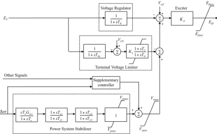
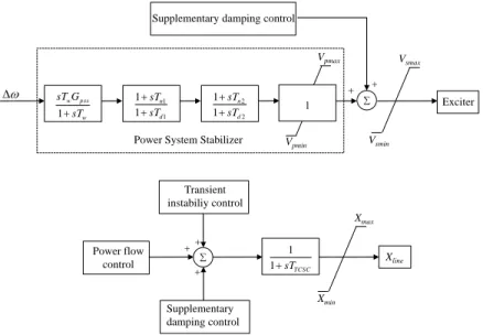
D C L _sT sT K + + 1 1 ∑ A K Exciter R sT + 1 1 ∑ Supplementary controller RL sT + 1 1 ∑ ∑ 2 2 1 1 d n sT sT + + 1 1 1 1 d n sT sT + + w pss w sT G sT + 1 1 Efmax Efmin Efd Vsmax Vsmin Vpmax Vpmin + + − + − Voltage Regulator Vref VLS

Terminal Voltage Limiter

ET

+ +

Power System Stabilizer ω

Δ Other Signals

+ −

Figure 2.3: Supplementary damping control

• It can infer good policies from relatively small samples of trajectories, even for some high-dimensional problems;

• Using a tree-based batch mode supervised learning technique [58] it solves the generalization problem associated with RL techniques in a generic way [57, 59].

2.2.5 Implementation strategy

The proposed trajectory-based control scheme is not intended to replace existing damping controllers, but rather to optimize some supplementary control signals and superimpose them on the outputs of existing damping controllers so as to improve damping effects. In this way, the adaptation and/or the coordination of these existing controllers is implicitly achieved. The implementation considered in our work is illustrated in Fig. 2.3. For a given generator, the supplementary controller adds its control signal at the output of the PSS of the generator; it uses as inputs the angular speed of the generator and possibly other remote signals such as active power flows over tie-lines, so as to help damping of oscillation modes other than local ones. At a control time, such a controller collects inputs and then it calculates the supplementary control signals so as to maximize the control return over a future temporal horizon.

(41)

2.3. THESIS CONTRIBUTIONS AND STRUCTURE 23

2.3 Thesis contributions and structure

2.3.1 Thesis contributions

Using the above proposed supplementary damping control approaches, the thesis attempts to design adaptive and coordinated damping control schemes based on the global information provided by WAMS and by leveraging recent progress in optimization and machine learning.

As the first step, a fully centralized MPC scheme is investigated (this work is reported in Chapter 4 and in our publication [60]). In this scheme, the MPC approach is implemented in a hypothetical system-wide control center and is responsible to compute supplementary inputs for all damping controllers so as to optimize their global control effects. It uses a linearized discrete-time state space model, calculates an optimal input sequence over a chosen time horizon by solving a quadratic programming problem. The first-stage control decision is applied to all controllers and the calculation is repeated at the subsequent measurement and control times. This scheme is firstly evaluated in ideal conditions: complete state observability and controllability, neglecting measurement errors and communication and computing delays. Next, the technical feasibility of this approach is assessed by studying also the effects of state-estimation errors, communication and computation delays and non-controllability of some local controllers. Finally, the scheme is tested to check if it can incorporate diverse damping controllers like PSS, TCSC and SVC, and efficiently coordinate them.

To design a damping control scheme more realistic in the context of large-scale interconnected power systems, the centralized MPC scheme is then re-placed by a distributed MPC scheme (Chapter 5, and our publication [61]). Considering information-exchange restrictions and organizational barriers in certain power grids, a large-scale power system is decomposed into some smaller control areas (subsystems) according to practical constraints. And then a MPC controller is set in each subsystem. Similar to the centralized MPC, a subsystem-wide MPC controller formulates its quadratic program-ming problem using a subsystem-wide model and control objective. It solves this problem to provide supplementary inputs for damping controllers under its authority. Each MPC controller tries to solve its own oscillation prob-lem and the overall system stability is hoped to result from these area-wise controls.

(42)

improve the robustness and reliability of damping control (Chapter 6, and our publication [62]). In addition to the MPC controllers working at the level of subsystems (the upper level), we set the new MPC controllers in the lower level consisting of local damping controllers. An upper MPC controller calculates supplementary inputs for all damping controllers under its author-ity, based on a subsystem model and subsystem-wide measurements. And it sends these inputs to lower MPC controllers as their control bases. The lower MPC controllers calculate, at a faster rate, corrections to the bases given by their corresponding upper MPC controllers, according to their own models, control objectives and measurements. Because the MPC controllers in the lower level only consider dynamics of one device like a generator or a transmission line, they need less time to measure, compute and apply their decisions. So, they can update more rapidly their control decisions following changes of local states, so as to approach better their control targets. The robustness of hierarchical MPC is tested using a larger refreshing interval at the upper level and incomplete measurements, considering controller and communication failures, and in different operation conditions.

Considering the possibility that system dynamics cannot be well enough approximated by a state space model at particular moments in practice, a model-free RL-based supplementary damping control is proposed in the sec-ond part of our research (Chapter 8, and our paper [63] under revision at the time of writing this manuscript). With the help of a tree-based batch mode RL, the control return of a candidate action at current state is approxi-mately calculated over a given temporal horizon, based only on dynamic and reward information collected from observed trajectories of power systems. The action with the largest return is superimposed on existing controller’s own output to improve damping effects. The scheme is first implemented on a single generator, and then several possibilities are investigated for extend-ing it to multiple generators. Finally the possible benefits of combinextend-ing this RL-based control with MPC are assessed.

2.3.2 Thesis structure

The thesis is organized as follows:

• Chapter 1 introduces power system electromechanical oscillations in terms of the definition, classification and consequences, and gives some oscillation examples in the European power system. Next,

(43)

mathemat-2.3. THESIS CONTRIBUTIONS AND STRUCTURE 25 ical insights into electromechanical oscillations are provided on a two-generator equivalent system. Electromechanical oscillation mechanisms and analysis methods are also discussed in this chapter. Finally, com-mon damping controls are shortly discussed.

• Chapter 2 presents research motivations, methods and contributions. The research objective is to design the optimized, adaptive and co-ordinated damping control scheme based on global dynamic

informa-tion. We define damping control as a Th-step optimal decision problem,

which can be solved by MPC or RL in a way of receding horizon. • In chapter 3, the underlying concept of MPC is described. Based on a

linearized, discrete and time-invariant state space model, MPC predic-tion equapredic-tions and objective funcpredic-tion are derived. We get a quadratic programming problem that can be solved by Active Set methods, Inte-rior Point methods, and so on. MPC stability and robustness must be carefully checked in practical applications. Finally, diverse MPC con-trol schemes are discussed to offer the reference for our MPC designs. • Chapter 4 focuses on a centralized MPC scheme for damping

electrome-chanical oscillations. It firstly describes the proposed centralized MPC scheme, and gives its mathematical formulations in ideal conditions. Next, it considers the effects of state-estimation errors, communica-tion and computacommunica-tion delays and non-controllability of local damping controllers. The scheme’s ability of incorporating diverse damping con-trollers is tested.

• Chapter 5 introduces a distributed MPC scheme which is considered to be more viable for damping low-frequency oscillations in very large-scale interconnected power systems. It discusses the decomposition of a large-scale power system, and formulates MPC for a subsystem based on a given decomposition. Then, it analyzes the coordination between subsystem-wise MPC controllers. Results of distributed MPC are compared with those of centralized MPC.

• Chapter 6 proposes a hierarchical MPC scheme that introduces the new lower MPC controllers on the basis of distributed MPC. It firstly outlines the hierarchical MPC scheme, and then discusses the coupling between two layers of MPC and the coordination between lower MPC

(44)

controllers. Finally, it investigates the robustness and computation efficiency of this hierarchical MPC scheme.

• Chapter 7 firstly introduces the concept of learning and three learning forms: supervised learning, unsupervised learning and reinforcement learning. The rest of this chapter focuses on reinforcement learning, whose definition, elements and elementary solutions are detailedly dis-cussed.

• Chapter 8 designs the supplementary damping control using a tree-based batch mode RL algorithm. It firstly describes this method in terms of extra-trees, fitted Q iteration and greedy decision making. Then it tests the method on a single generator, and multiple generators. Finally the combination between MPC and RL is investigated.

• Chapter 9 offers some conclusions and discusses some further works. • Detailed information about the simulation tool and test system used

for our investigations can be found in the appendices.

2.4 Summary

This chapter introduced our research motivation, namely to improve damp-ing effects of existdamp-ing controllers by usdamp-ing global information, and by adap-tively adjusting and coordinating them. For this purpose, a trajectory-based supplementary damping control approach is proposed, considering the latest advances in power systems, machine learning and large-scale optimization, to compute supplementary inputs to superimpose on existing controllers to adjust and coordinate them. This approach aims at forcing the controlled system dynamics to evolve approximately along a desired trajectory, so as to damp electromechanical oscillations, with the help of certain supplementary control inputs. Mathematically, it is described as a Th-step optimization

con-trol problem, which could be solved either by MPC or by RL. Finally, the contributions and structure of this thesis are listed.

(45)

Part II

Model predictive control for

damping inter-area oscillations

of large-scale power systems

(46)

(47)

Chapter 3 Model predictive control

background

The content of the present chapter is adapted from [49, 64, 65]. Before pre-senting our MPC-based damping schemes, MPC’s theoretical knowledge [49], advantages [64] and available control structures [65] are provided in order to make the thesis self-contained.

3.1 What is MPC ?

The principle of MPC can be shortly summarized as follows. At any time, the MPC algorithm uses the collected measurements, a model of the system and a specification of the control objective to compute an optimal open-loop control sequence over a specified time horizon. The computed optimal first-stage controls are applied to the system. At the next time step, as soon as measurements (or model) updates are available, the entire procedure is repeated by solving a new optimization problem with the time horizon shifted one step forward [49]. The MPC technology was originally developed for power plant and petroleum refinery applications, but can now be found in a wide variety of manufacturing environments including chemicals, food processing, automotive, aerospace, metallurgy, pulp and paper [64].

The basic idea of MPC for a single-input single-output system is shown in Fig 3.1 [49]. We assume a discrete-time setting, and that the current time is labeled as time step k. The set-point trajectory s[t] is the trajectory

that the real output y[t] should follow. The solid line yref[t|k] is termed

(48)

s[t] y[t] k K+Th Time ŷ[t|k] k K+Th Time Input Th y_ref[t|k] Output

Figure 3.1: The basic idea of MPC. Taken from [49]

the reference trajectory, which starts at the current system output y[k|k], and defines an ideal trajectory along which the system should return to the set-point trajectory.

At time k, a predictive controller collects current state ˆx[k|k] and

calcu-lates the optimal input trajectory ˆu[k + i|k] using a dynamic system model,

in order to obtain the best possible future behavior ˆy[k + i + 1|k] with respect to a reference trajectory yref[k + i + 1|k], over a given prediction horizon Th,

i = 0, 1, ..., Th− 1. A cost function is defined to assess what is the optimal

sequence of inputs. In this example, ˆu[k + i|k] varies over the first Tc steps,

but remains constant thereafter. So the control horizon Tc is 3.

Once a future input trajectory ˆu[k + i|k] is chosen, only the first element of the trajectory ˆu[k|k] is applied as the real input u[k|k] to the system. Then the whole cycle of measurement, prediction, and input trajectory

determi-nation is repeated at subsequent refreshing times: a new ˆx[k + 1|k + 1] is

obtained; a new reference trajectory yref[k +1+i|k +1] is defined; predictions

are made over the time horizon Th; a new input trajectory ˆu[k + 1 + i|k + 1]

is chosen, and finally the first input ˆu[k + 1|k + 1] is applied to the system. The success of MPC technology can be attributed to three important fac-tors [64]. The first and foremost is the incorporation of an explicit process

(49)

3.2. MATHEMATICAL FORMULATION OF MPC 31 model into the control calculation. This allows MPC, in principle, to deal directly with all significant features of process dynamics. Secondly the MPC algorithm considers system behaviors over a future temporal horizon. This means that the effects of feedforward and feedback disturbances can be an-ticipated and removed, to drive the controlled system to evolve more closely along a desired future trajectory. Finally the MPC controller considers pro-cess input, state and output constraints directly in the control calculation. This means that constraint violations are far less likely, resulting in tighter control at the optimal constrained steady-state.

3.2 Mathematical formulation of MPC

In the present section MPC’s prediction equations, objective functions and constraints are formalized based on a linearized, discrete and time-invariant state space model in the form:

x[k + 1|k] = Ax[k|k] + Bu[k|k] y[k|k] = Cyx[k|k]

z[k|k] = Czx[k|k],

(3.1)

where x is a dx-dimensional state vector, u is a du-dimensional input vector,

y is a dy-dimensional vector of measured outputs, and z is a dz-dimensional

vector of outputs which are to be controlled, either to particular set-points, or to satisfy some constraints, or both. The index k counts ‘time steps’. The variables in y and z usually overlap to a large extent, and frequently they are the same. That is to say, all the controlled outputs are frequently measured.

So, we assume that y ≡ z, and we use C to denote both Cy and Cz. The

Eqn. (3.1) can thus be rewritten as:

x[k + 1|k] = Ax[k|k] + Bu[k|k]

y[k|k] = Cx[k|k]. (3.2)

In practice, we shall not assume that all state variables can be measured directly and exactly, so we use an estimated ˆx[k|k] instead of the real state x[k|k]. Correspondingly, ˆx[k + 1|k] and ˆy[k + 1|k] denote the predictions of

Distributed control of electromechanical oscillations in very large-scale electric power systems

UNIVERSITY OF LIEGE

DEPARTMENT OF ELECTRICAL ENGINEERING

AND COMPUTER SCIENCE

DISTRIBUTED CONTROL OF

ELECTROMECHANICAL OSCILLATIONS

IN VERY LARGE SCALE ELECTRIC

POWER SYSTEMS

BY

DA WANG

SUBMITTED IN PARTIAL FULFILLMENT OF THE

REQUIREMENT FOR THE DEGREE OF DOCTOR

OF PHILOSOPHY IN ENGINEERING SCIENCE

DOCTORAL THESIS

Abstract

Acknowledgments

List of acronyms and symbols

Acronyms

Symbols

Contents

I

Introduction

1

II

Model predictive control for damping inter-area

oscillations of large-scale power systems

27

III

Reinforcement Learning Based Supplementary

Damping Control

83

IV

Conclusions and future work

113

V

Appendices

119

Part I

Introduction

Chapter 1

Power system

electromechanical oscillations

1.1

Oscillation modes

1.2

Mathematical formulations

1.3

Electromechanical oscillation mechanisms

1.3.1

Negative damping

1.3.2

Other causes

1.4

Analysis methods

1.4.1

Linear methods (adapted from [1])

1.4.2

Nonlinear methods

1.4.3

Signal analysis methods

1.5

Controllers and actuators

1.5.1

PSS

1.5.2

FACTs devices

1.5.3

HVDC modulation

1.6

Conclusions

Chapter 2

Research motivations, methods

and contributions

2.1

Research motivations

2.2

Trajectory-based supplementary control

2.2.1

Feasibility

2.2.2