HAL Id: hal-01703140
https://hal.archives-ouvertes.fr/hal-01703140
Submitted on 22 Feb 2018
HAL is a multi-disciplinary open access
archive for the deposit and dissemination of
sci-entific research documents, whether they are
pub-lished or not. The documents may come from
teaching and research institutions in France or
abroad, or from public or private research centers.
L’archive ouverte pluridisciplinaire HAL, est
destinée au dépôt et à la diffusion de documents
scientifiques de niveau recherche, publiés ou non,
émanant des établissements d’enseignement et de
recherche français ou étrangers, des laboratoires
publics ou privés.
Predictive models of hard drive failures based on
operational data
Nicolas Aussel, Samuel Jaulin, Guillaume Gandon, Yohan Petetin, Eriza Fazli,
Sophie Chabridon
To cite this version:
Nicolas Aussel, Samuel Jaulin, Guillaume Gandon, Yohan Petetin, Eriza Fazli, et al.. Predictive
models of hard drive failures based on operational data. ICMLA 2017 : 16th IEEE International
Conference On Machine Learning And Applications, Dec 2017, Cancun, Mexico.
pp.619 - 625,
Predictive Models of Hard Drive Failures
based on Operational Data
Nicolas Aussel
∗†, Samuel Jaulin
∗†, Guillaume Gandon
∗†, Yohan Petetin
†, Eriza Fazli
∗and Sophie Chabridon
†∗Zodiac Inflight Innovations, Wessling, Germany
†SAMOVAR, T´el´ecom SudParis, CNRS, Universit´e Paris-Saclay, France
Abstract—Hard drives are an essential component of modern data storage. In order to reduce the risk of data loss, hard drive failure prediction methods using the Self-Monitoring, Analysis and Reporting Technology attributes have been proposed. How-ever, these methods were developed from datasets not necessarily representative of operational systems. In this paper, we consider the Backblaze public dataset, a recent operational dataset from over 47,000 drives, exhibiting hard drive heterogeneity with 81 models from 5 manufacturers, an extremely unbalanced ratio of 5000:1 between healthy and failure samples and a real-world loosely controlled environment. We observe that existing predictive models no longer perform sufficiently well on this dataset. We therefore selected machine learning classification methods able to deal with a very unbalanced training set, namely SVM, RF and GBT, and adapted them to the specific constraints of hard drive failure prediction. Our results reach over 95% precision and 67% recall on a one year real-world public dataset of over 12 million records with only 2586 failures.
I. INTRODUCTION
Hard drives are essential for data storage but they are one of the most frequently failing components in modern data centres [1], with consequences ranging from temporary system unavailability to complete data loss. Many predictive models, analysed in section II, have already been proposed to mitigate hard drive failures but failure prediction in real-world operational conditions remains an open issue. One reason is that some failures might not be predictable in the first place, resulting, for example, from improper handling happening occasionally even in an environment maintained by experts. However, this alone cannot explain why the high performances of the failure prediction models that appear in the literature have not mitigated the problem further. Therefore, the speci-ficities of hard drives need to be better taken into account.
First of all, the high reliability of a hard drive implies that failures have to be considered as rare events which leads to two difficulties. The ideal application case of many learning methods is obtained when the classes to predict are in equal proportions. Next, it is difficult to obtain sufficient failure occurrences. Indeed, hard drive manufacturers themselves pro-vide data on the failure characteristics of their disks but it has been shown to be inaccurate (see e.g. [1], [2]) and often based on extrapolating from the behaviour of a small population in an accelerated life test environment. For this reason, it is important to work with operational data collected over a large period of time to ensure that it contains enough samples of hard drive failures.
Another challenge is that the Self-Monitoring, Analysis and Reporting Technology (SMART) used to monitor hard drives is not completely standardized. Indeed, the measured set of attributes and the details of SMART implementation are different for every hard drive manufacturer. From a machine learning point of view, there is no guarantee that a learning model trained to predict the failures of a specific hard drive model will be able to accurately predict the failures of another hard drive model. For this reason, in order to draw conclusions on hard drive failure prediction in general, it is important to ensure that the proposed predictive models are estimated from a variety of hard drive models from different manufacturers and also tested on a variety of hard drive models. Until now, this constraint was not taken into account properly, probably because gathering a representative dataset has been a problem for many previous studies, impairing the generality of their conclusions. We rather focus on the Backblaze public dataset1 consisting of several years worth of measurements
on a large drive population operated in an expert-maintained environment. It has been made available recently, with the earliest measurements done in 2013.
The objective of this paper is to offer an insight as to why many previous studies are not directly applicable when considering class imbalance, data heterogeneity and data vo-lume and next to adapt predictive models based on machine learning methods for pattern recognition of hard drive failure prediction. We also compare the proposed models and discuss their performances on the Backblaze dataset that includes hard drives from different manufacturers in order to determine if they are robust to the differences in SMART parameters. The paper is organized as follows. In section II, we review the state-of-the-art while paying a particular attention to the datasets that were used. In section III, we detail the new dataset that we use for this study and the specific challenges associated with it. In section IV, we describe the different machine learning techniques that we applied to the dataset, and we underline the different steps of pre-processing, feature selection, sampling, learning and post-processing. In section V, we present and discuss our experimental results obtained with the three most relevant learning models: Support Vector Machine (SVM), Random Forest (RF) and Gradient-Boosted Tree (GBT). Finally, we end the paper with a conclusion and we discuss possible ways to extend this study.
II. RELATEDWORK
Several studies on the subject of hard drive failure prediction based on SMART data have already been carried out. [3], [4], [5] and [6] all used the same dataset. The models were tested on a dataset of 369 hard drives of the same model with healthy drives and failed drives in equal proportions. The data from healthy drives was collected in a controlled environment by the manufacturer. In [3], several methods are proposed to build a prediction model: SVM, unsupervised clustering, rank-sum test and reverse arrangements test. This study found the best method among those tested to be the rank-sum test by detecting 24% of the failed drives while maintaining a false alarm rate below 1%. In [4], a subsequent study from the same authors, the best performances were obtained with a SVM with a detection rate of 50.6% and a false alarm rate below 0.1%. In [5], hidden Markov models and hidden semi-Markov models are tested. The best model reaches a detection rate of 52% and a false alarm rate below 0.1%. In [6], a health monitoring method based on the Mahalanobis distance is developed. It yields a detection rate of 67% while maintaining the false alarm rate below 0.1% still.
In [7], two Bayesian methods are tested, a Bayesian clus-tering model based on expectation maximization and a super-vised naive Bayes classifier. The dataset used was collected from 1927 drives including 9 failed drives. The performances reached are 60% detection rate and a false alarm rate of 0.5%. In [8] and [9], a dataset comprising samples from 23, 395 drives operating in a data center is studied. Two different hard drives models from the same manufacturer are used. The methods used are back-propagation recurrent neural networks, SVM, classification and regression trees. The best results are obtained with classification trees achieving over 95% detection with a false alarm rate of 0.09%.
In [10], a population of 1, 000, 000 drives is studied. 6 hard drive models are considered. The method used is threshold-based classification with only 1 SMART parameter. It reaches 70.1% recall and 4.5% false alarm rate. The dataset is unfor-tunately not publicly available.
As we see, most previous studies were conducted have been led on small datasets collected in a controlled environment using manufacturer data. Moreover, [1] and [2] have shown that manufacturer data on disk reliability is not accurate as it is relying on accelerated life tests and stress tests that appear to consistently underestimate the actual disk failure rate. As such, hard drive failure prediction models trained on manufacturer data have a high risk of being biased and cannot be relied on. Additionally, in [3] manufacturer data on hard drives is mixed with data from hard drives returned by users. The authors highlight in their paper the importance of understanding the induced limitations. However, given how often this dataset is used in other studies such as [5] or [6], it is preferable to rely on a dataset without such mixing.
The most notable exceptions to these issues are the stu-dies [8] and [9]. Unfortunately the associated dataset used is not publicly available and is limited to two drive models.
Very recently, some studies started to exploit the Back-blaze dataset. [11] considers a large subset of over 30, 000 drives from the Backblaze dataset to train several classifiers. However, the results (98% for the detection and 98% for the precision) are obtained on a limited and different subset of filtered data. In the industry, [12] shows promising results but the lack of implementation details prevents comparison.
Another limitation of previous studies is the choice of evaluation metrics which generally coincide with the detection and false alarm rates. This is a relevant choice for balanced datasets but, as operational datasets are extremely unbalanced in favour of healthy samples, even a low false alarm rate in the range of 1% could translate into poor performances. Therefore, we rather report precision and recall metrics.
In order to overcome these issues related to the dataset and to provide reproducible results, we consider a large, operational and publicly available dataset from Backblaze, and compute the precision and recall metrics, rather than detection and false alarm rates, on unfiltered samples. This enables us to draw conclusions for operational data.
III. DATASET
This work relies on operational data that the Backblaze company started to release at the end of 2013. It gathers daily measurements of SMART parameters of each operational hard drive disk of this company data centre. Updates to the dataset are provided quarterly. The fields of the daily reports are composed as follows: the date of the report, the serial number of the drive, the model of the drive, the capacity of the drive in bytes, a failure label that is at 0 as long as the drive is healthy and that is set to 1 when the drive fails and finally the SMART parameters. For the rest of the study, we focus on the data from January 2014 to December 2014 in order to enable a comparison between prediction performances. Over this period, 80 fixed SMART parameters are collected among those defined by the manufacturers. They include, for example, counts of read errors, write faults, the temperature of the drive and its reallocated sectors count. However, it should be noted that most drives do not report every parameter resulting in many blank fields. The reason why is that hard drive disk manufacturers are free to decide how to implement SMART parameters. For the same reason, there is no guarantee that SMART parameters from two different models or manufacturers have the same meaning since the details of their implementation are not disclosed.
Finally, the dataset contains over 12 million samples from 47, 793 drives including 81 models from 5 manufacturers. Among those 12 million samples, only 2, 586 have their failure labels set to 1 and the others are healthy samples, for an overall ratio of about 2 failure samples for every 10, 000 healthy samples that is below 0.022%.
IV. DATA PROCESSING
We identify in this section a set of classification techniques that are best suited for an extremely unbalanced training set and a loosely controlled environment in real operation as
opposed to laboratory experimentations. Considering the size of the dataset, we focus on classification computations that can be distributed across several nodes. Roughly speaking, we have at our disposal a set of multidimensional observations x ∈ Rd, (x1, x2, ..., xd). For example, x may represent the SMART
parameters or a transformation of the SMART parameters. For a given x, we associate a label y ∈ {0, 1}. The goal of the classification is to determine a function that given a sample x associates a label y that matches the failure label of the dataset.
A. Pre-processing
As noted in [2], traditionally used outlier filtering techniques such as Extreme Value Filtering are inadequate for SMART values of an operational set as it is difficult to distinguish between exceptional values caused by a measurement artefact or by an anomalous behaviour that may lead to a hard drive failure. A classical approach is to limit filtering to obvious errors. In our case, this corresponds to physically impossible values such as power-on hours exceeding 30 years. We filter on two SMART parameters, SMART 9, power-on hours, and SMART 194, temperature. In turned out that this filtering is negligible and does not noticeably impact the dataset with only 5 drives concerned, matching the observation in [2] that less than 0.1% of the hard drives are concerned.
Similarly to what is done in [8], we define a time window for failure in the following manner: after a drive fails, we relabel a posteriori the N previous samples from this particular drive as failures where N is the length of the time window in days. In other words, with our classification model we try to answer the question ”Is the hard drive going to fail in the next N days?”. This length will be optimized as a hyper parameter of the model to determine its optimal value if it exists. B. Feature selection
Not every SMART parameter is indicative of a failure [2]. As such, we consider different strategies for feature selection. The main one is based on the pre-selection used in [2], [8], [9] of SMART parameters highly correlated to failure events. With this scheme, we consider only the nine raw SMART parameters number 5, 12, 187, 188, 189, 190, 198, 199 and 200.
Some models such as Random Forests are not vulnerable to noisy features and are, in fact, able to extract information from features with low correlation with failure events. This also provides the additional benefit of not relying on sources external to the dataset to select the features. When it is relevant, we thus train these models on the complete set of features.
C. Sampling techniques
In order to reduce the impact of the class imbalance issue on the learning algorithms, we investigated the use of sam-pling techniques. Given the extreme imbalance factor of the dataset, naive oversampling and undersampling were excluded as potential sources of overfitting [13]. Contrary to [11], we
limit the application of sampling techniques to the same subset of data used for training.
SMOTE (Synthetic Minority Oversampling Technique) aims at alleviating class imbalance by generating additional training samples of the minority class through interpolation [14]. SMOTE first selects a random minority sample, then de-termines its k nearest neighbours, selects one of them and places randomly on the segment between the two samples a new artificial minority sample. This process is then repeated as many times as necessary before reaching a pre-selected oversampling factor. By creating artificial instances distinct from the existing minority samples, it partially avoids the overfitting problem observed with naive oversampling.
Another step to improve the training set is to filter a certain category of failure samples. We observe that some failure samples share the exact same feature values as healthy samples leading to the impossibility for any classifier based on those features to discriminate them. Thus, filtering those hard-to-classify failure samples leads to a trade-off of a higher precision at the expense of recall.
D. Machine Learning algorithms
Previous studies such as [11] have considered Logistic Regression (LR) for hard drive failure prediction. We imple-mented it but results show a constant prediction in favour of the majority class, which is understandable given the sensitivity of LR to class imbalance. Further work on sampling techniques is needed in order to use LR on the Backblaze dataset. We therefore focus our experimentations on solutions able to deal with extreme class imbalance.
Support Vector Machine (SVM) is a technique that re-lies on finding the hyperplane that splits the two classes to predict while maximizing the distance with the closest data points [15]. We use a linear kernel in order to enable parallelization of the computations. With N the number of samples, xi the features of a sample, y its label and ~w the
normal vector to the hyperplane considered, b the hyperplane offset and λ he soft-margin, the SVM equation to minimize is: f ( ~w, b) = λk ~wk2+ 1 N N X i=1 max(0, 1 − yi(w.xi− b)) (1)
It is optimized through 100 steps of stochastic gradient de-scent.
Random Forest (RF) is an ensemble technique based on a decision tree classifier. A decision tree works by splitting the data set into smaller subsets based on measured attributes until either the subsets are each composed of only one class or the maximum depth of the tree has been reached. RF improves on this technique by combining several decision trees each trained on bootstrapped samples with different attributes. New predictions are then made based on a vote among the different decision trees [16]. The loss function minimized for each split is as follow: given m the current node to split, Qm the data
available at that node, Nm the number of samples in Qm,
split respectively to the left and right of the node and H the impurity function, nlef t Nm H(Qlef t(θ)) + nright Nm H(Qright(θ)) (2)
This step is repeated until Nm = 1 or the maximum depth
is reached. In this study, we set the number of decision trees at 50 with a maximum depth of 8, constructed using the Gini impurity metric.
Finally, Gradient boosted tree (GBT) is another ensemble technique based on decision trees. Instead of training random trees like in RF, the training takes place in an iterative fashion with the goal of trying to minimize a loss function using a gradient descent method [16]. In this study, the initial splits are done using the same equation as the RF trees and the iterations are done with a log loss function characterized by the formula: 2 ×PN
i=1log(1 + exp(−2yiF (xi))) where N
is the number of samples, xi and yi respectively the features
and the label of the sample i and F (xi) the predicted label
for sample i. This function is minimized through 10 steps of gradient descent.
All the parameters of the learning methods are optimized through grid-search.
V. EXPERIMENTAL RESULTS
A. Post-processing
In order to ensure the accuracy of the results, two additional steps are taken. First, we perform cross-validation through a customized stratified k-folding algorithm. The samples are first regrouped by HDD serial number so that the samples measured on one HDD are always in the same fold. HDDs are then split between those that reported a failure during the study and those that did not. The stratified k-sampling then takes place on the HDD level and not on the individual sample level in order to ensure that samples from a given HDD are always in the same fold. For this study, the number of folds has been fixed to 3. On top of that, in order to account for the optimization of the length of the time-window as an hyper-parameter of the models, every measurement is rerun three times by selecting new sets of folds for the cross-validation and the mean value is reported.
Two metrics are measured on the failed samples, precision and recall respectively defined as the number of successfully predicted failures divided by the total number of predictions and the number of failures successfully predicted divided by the total number of failures observed. If we define the failure sample as positive and the healthy samples as negative we have:
precision = true positive
true positive + f alse positive (3) recall = true positive
true positive + f alse negative (4) Note that contrary to similar studies referenced in section II, we decide to report precision instead of false alarm rate: due to the high class imbalance, even a small false alarm rate could
translate into poor performances. Indeed, a misclassification of only 1% of the healthy samples would result in 100 false alarms for every 10, 000 healthy samples, on average; since there are only 2 failure samples for every 10, 000 healthy samples, it means that we have 50 false alarms for every detected failure if we assume 100% recall on the failure samples, and consequently a precision below 2%. Similarly, we can note that a constant prediction in favour of the majority class would result in an accuracy of 99.98%.
B. Results and discussion
The performances in terms of precision and of recall are displayed in Fig. 1 (SVM), Fig. 2 (RF) and 3 (GBT) as a function of the time window length.
The SMOTE sampling strategy is then tested on the best performing model, RF with all features.
The experimental setup we use is a cluster of 3 computers running Apache Spark v2.1 using a total of 24 cores. Due to the various size of the time window parameter, cross-validation and repetition of the tests, every technique is run a total of 180 times, not including the grid-search executions to optimize the parameters. The execution time is reported in Table I.
Method Execution time (1 run) Execution time (180 runs) SVM preselected 11 min 33 hours
SVM all features 24 min 72 hours GBT preselected 10 min 30 hours GBT all features 41 min 123 hours RF preselected 14 min 42 hours RF all features 37 min 111 hours RF+SMOTE 42 min 126 hours
TABLE I
EXECUTION TIME OF THE METHODS
There are several interesting points to notice on the graphs. First, on figure 1 for the linear SVM, we note that the perfor-mances are low. This is likely a sign that the classes to predict are not linearly separable. The solution for this would be to use another kernel for the SVM but unfortunately this would be at the cost of the parellelization of the implementation which would push the computation time beyond acceptable range. Regarding the length of the time window, it should be noted that the linear increase in precision with preselected features is likely only a side-effect of the relabelling. Further investigation reveals that the support vectors are not changing when the time window changes so the model learnt is the same. This is most likely because the inertia of the SVM model is too high to be affected by changing less than 0.1% of the labels.
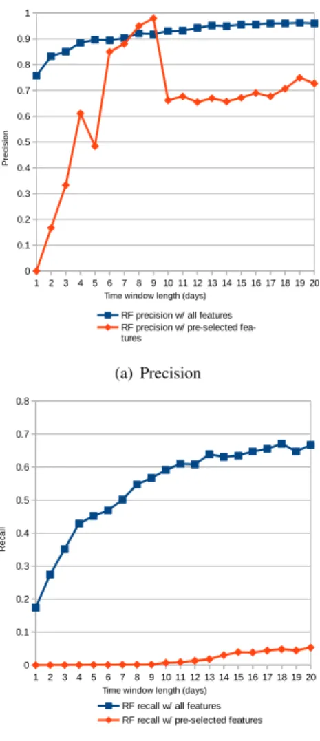
Second, for RF, on figure 2, we can note that the usage of pre-selected features does not improve the performances but decreases them. The fact that feature selection does not bring improvement is understandable given that RF models have been shown to be resilient to noisy features. However the decrease also implies that the features that were not pre-selected are not pure noise but also contain useful information to predict an impending failure. This highlights the fact that SMART features are implemented differently on different drives and thus that conclusion regarding features useful for
(a) Precision
(b) Recall
Fig. 1. Precision and Recall of SVM for two feature selection modes and varying time window length
predicting failures of a specific type of hard drive model cannot easily be generalized to every type of hard drive. Additionally, for small values of the time window, the RF model struggles because the scarcity of the failure labels is further aggravated by the bagging technique used to learn the individual decision trees that compose the RF model. This is especially true with the pre-selected features.
Finally, for GBT, on figure 3 it does not display the same limitation as RF for time windows higher than one day, likely because it is not based on a bagging technique. The performances when using all available features are mostly similar to RF.
Overall, the best performances are reached by RF and GBT when using all available features with RF reaching up to 95% precision and 67% recall and GBT reaching up to 94% precision and 67% recall. The reported precision of 95% and 94% would translate on average with daily measurements on a single hard drive into a single false alarm respectively every 100.000 days and 83.333 days. In the mean time, over two thirds of the failures would be predicted correctly.
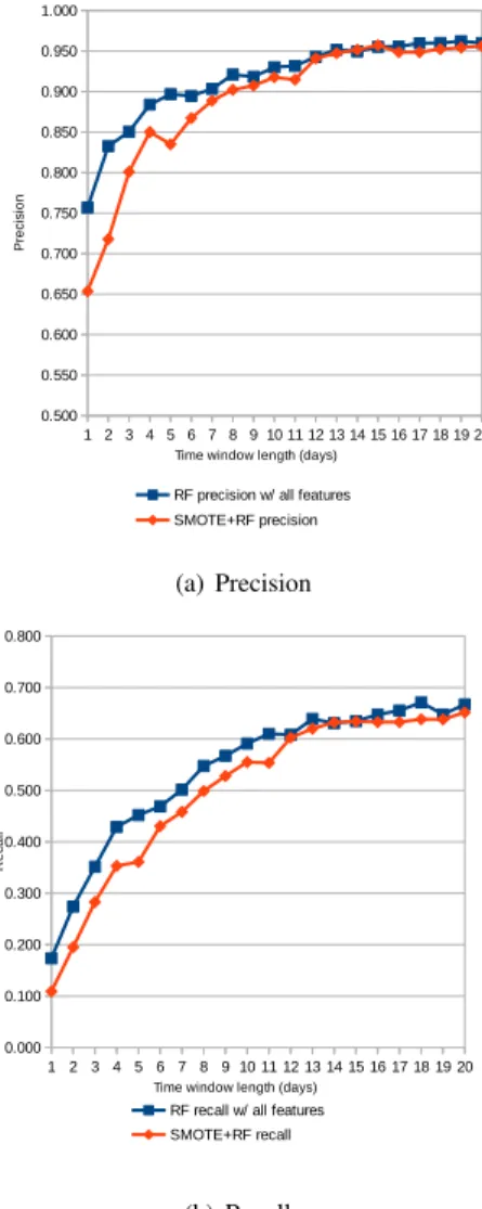
In table 4, the last experiment with the SMOTE sampling
(a) Precision
(b) Recall
Fig. 2. Precision and Recall of RF for two feature selection modes and varying time window length
technique resulted in negative results. The precision and recall of RF are decreased by SMOTE for smaller values of the time window and are similar at higher values. This is likely the result of an imbalance factor of 5000, much higher than the one used when developing sampling techniques which remains in the range of 2 to 100 [17].
VI. CONCLUSION
In this paper, we work on hard drive failure prediction with a publicly available, large and operational dataset from Backblaze with relevant metrics, which is crucial to bridge the gap between laboratories studies and real-world systems and for reaching reproducible scientific results. This implies to address the class imbalance between failures and non-failures and the large dataset size. We have selected the precision and recall metrics, most relevant to the problem, and tested several learning methods, SVM, GBT and RF. With 95% precision and 67% recall, the best performances were provided by RF with all features while GBT was a close contender with 94% precision and 67% recall. SVM performances were
(a) Precision
(b) Recall
Fig. 3. Precision and Recall of GBT for two feature selection modes and varying time window length
unsatisfactory with a precision below 1%. We have also shown that when studying different hard drive models from different manufacturers, selecting the features classically used for hard drive failure prediction leads to a drop in performances.
Contrary to what was expected, SMOTE did not improve the prediction performances highlighting the difficulties stemming from the extreme unbalanced ratio of the Backblaze dataset. Additional work on sampling techniques is needed to balance the dataset. Ensemble-based Hybrid sampling techniques [17] such as SMOTEBagging, an improvement of the SMOTE sampling technique, could help to improve our learning models and might enable to use learning methods more sensitive to class imbalance such as logistic regression.
Finally, we plan to evaluate on the Backblaze dataset other learning techniques which have demonstrated promising results on other samples such as back-propagation recurrent neural networks [8], Bayesian classifiers [7] or Mahalanobis distance [6].
(a) Precision
(b) Recall
Fig. 4. Precision and Recall of the RF model for varying time window length with and without SMOTE sampling
REFERENCES
[1] B. Schroeder and G. A. Gibson, “Disk Failures in the Real World: What Does an MTTF of 1,000,000 Hours Mean to You?” in 5th USENIX Conf. on File and Storage Technologies, ser. FAST ’07. Berkeley, CA, USA: USENIX Association, 2007.
[2] E. Pinheiro, W.-D. Weber, and L. A. Barroso, “Failure Trends in a Large Disk Drive Population,” in FAST, vol. 7, 2007, pp. 17–23.
[3] J. F. Murray, G. F. Hughes, and K. Kreutz-Delgado, “Hard Drive Failure Prediction using Non-parametric Statistical Methods,” in ICANN/ICONIP, 2003.
[4] ——, “Machine learning methods for predicting failures in hard drives: A multiple-instance application,” J. Mach. Learn. Res., vol. 6, pp. 783– 816, Dec. 2005.
[5] Y. Zhao, X. Liu, S. Gan, and W. Zheng, “Predicting Disk Failures with HMM-and HSMM-based Approaches,” in Industrial Conf. on Data Mining. Springer, 2010, pp. 390–404.
[6] Y. Wang, Q. Miao, and M. Pecht, “Health monitoring of hard disk drive based on Mahalanobis distance,” in Prognostics and System Health Managment Conf., May 2011, pp. 1–8.
[7] G. Hamerly and C. Elkan, “Bayesian Approaches to Failure Prediction for Disk Drives,” in 18th Int. Conf. on Machine Learning, 2001. [8] B. Zhu, G. Wang, X. Liu, D. Hu, S. Lin, and J. Ma, “Proactive Drive
Failure Prediction for Large Scale Storage Systems,” in IEEE 29th Symp. on Mass Storage Systems and Technologies, May 2013, pp. 1–5.
[9] J. Li, X. Ji, Y. Jia, B. Zhu, G. Wang, Z. Li, and X. Liu, “Hard Drive Failure Prediction using Classification and Regression Trees,” in 44th IEEE/IFIP Conf. on Dependable Systems and Networks, June 2014. [10] A. Ma, R. Traylor, F. Douglis, M. Chamness, G. Lu, D. Sawyer,
S. Chandra, and W. Hsu, “RAIDShield: Characterizing, Monitoring, and Proactively Protecting Against Disk Failures,” ACM Trans. on Storage, Special issue FAST’2015, vol. 11, no. 4, pp. 17:1–17:28, Nov. 2015. [11] M. M. Botezatu, I. Giurgiu, J. Bogojeska, and D. Wiesmann,
“Predict-ing Disk Replacement Towards Reliable Data Centers,” in 22d ACM SIGKDD Conf. on Knowledge Discovery and Data Mining, 2016. [12] A. El-Shimi, “Predicting Storage Failures,” in VAULT - Linux Storage
and File Systems Conference, Cambrige (MA), Mar. 2017. [Online]. Available: http://events.linuxfoundation.org/sites/events/files/slides/LF-Vault-2017-aelshimi.pdf
[13] B. C. Wallace, K. Small, C. E. Brodley, and T. A. Trikalinos, “Class Imbalance, Redux,” in IEEE 11th Conf. on Data Mining, Dec 2011. [14] N. V. Chawla, K. W. Bowyer, L. O. Hall, and W. P. Kegelmeyer,
“SMOTE: synthetic minority over-sampling technique,” Journal of arti-ficial intelligence research, vol. 16, pp. 321–357, 2002.
[15] C. Cortes and V. Vapnik, “Support-vector networks,” Machine Learning, vol. 20, no. 3, pp. 273–297, 1995.
[16] A. Criminisi, J. Shotton, and E. Konukoglu, “Decision Forests: A Unified Framework for Classification, Regression, Density Estimation, Manifold Learning and Semi-Supervised Learning,” Foundations and Trends in Computer Graphics and Vision, vol. 7, no. 23, pp. 81–227, 2012. [17] M. Galar, A. Fernandez, E. Barrenechea, H. Bustince, and F. Herrera,
“A Review on Ensembles for the Class Imbalance Problem: Bagging, Boosting, and Hybrid-Based Approaches,” IEEE Trans. on Systems, Man, and Cybernetics, vol. 42, no. 4, pp. 463–484, July 2012.