The Wild Bootstrap for the Variance Radio Test

Universit´e de Montr´eal

The wild bootstrap for the Variance Ratio test

par Rong Luo

Directrice de recherche: Silvia Gon¸calves

D´epartement de sciences ´economiques

Facult´e des arts et des sciences

Rapport pr´esent´e `a la Facult´e des ´etudes sup´eieures en vue de l’obtention du

grade de M.Sc. en Sciences ´

Economiques (2-240-1-0)

option ´

Economie financi`ere

Abstract

This paper discusses the wild bootstrap for the Variance Ratio test. Under heteroskedasticity of unknown form, a properly designed wild bootstrap method applied to the Variance Ratio test shows better performance than the traditional asymptotic test. One of our main goals is to study the impact of the form of the re-centering on the finite sample properties of the bootstrap Variance Ratio statistic. The size and the power of different tests are compared using the popular volatility models used in finance.

Contents

1 Introduction 2

2 The Variance Ratio statistic 3

3 The bootstrap Variance Ratio statistic 4

4 Simulation results 6

4.1 The empirical distributions . . . 6

4.2 The size of the tests . . . 7

4.3 The power of the tests . . . 8

5 Conclusion 19

List of Figures

List of Tables

2 Empirical size of asymptotic test, Lo and Mackinlay’s (1988) approach (α = 0.05) . . 15

3 Empirical size of WB test, center around 1, Kim’s (2006) approach (α = 0.05) . . . . 15

4 Empirical size of WB test, center around VR (α = 0.05). . . 16

5 Empirical size of WB test, center around 1, based on symmetric confidence intervals (α = 0.05) . . . 17

6 Power of the asymptotic test . . . 17

7 Power of the WB test, based on equal-tailed confidence intervals . . . 18

1

Introduction

Variance Ratio (henceforth VR) statistics are very used in empirical finance and economics for testing the null hypothesis of a random walk. For example, Liu and He (1991), Ayadi et al. (1994), Fong et al. (1997) and Yilmaz (2003) evaluated the martingale property in exchange rates. The use of the VR test for the martingale hypothesis of stock prices include Lo and MacKinlay (1988), Kim et al. (1991), Frennberg and Hansson (1993), and Malliaropulos and Priestley (1999). Typically VR tests are based on the first order asymptotic theory as de-veloped by Lo and MacKinlay (1988). Because financial data is characterized by conditional heteroskedasticity of unknown form, it is important to use a heteroskedasticity consistent vari-ance estimator. Lo and MacKinlay (1988) propose such an estimator. Existing simulation results show that the asymptotic theory is a poor approximation to the true finite sample distribution of the VR statistic. For example, Lo and MacKinlay (1989) found that the sampling distribu-tion of their VR statistic can be very different from the standard normal distribudistribu-tion in small samples, with severe bias and right skewness. This can lead to size distortions or low power in small samples, resulting in misleading statistical inference.

In this paper we consider the bootstrap for VR statistics. Our main motivation is to improve upon the first order asymptotic theory of Lo and MacKinlay (1988). In particular, we focus on the wild bootstrap (henceforth WB) for VR statistics. The WB was introduced by Wu (1986) to handle unconditional heteroskedasticity in linear regression models and further studied by Mammen (1993). Recently, Goncalves and Kilian (2004) proved the first order asymptotic valid-ity of the WB in the context of linear dynamic regression models whose errors are conditionally heteroskedastic. In our context, the WB is robust to conditional heteroskedasticity of unknown form, often present in financial data.

Interestingly, not many papers have considered the bootstrap for VR statistics. One exception is Kim (2006), who also studies the finite sample properties of the WB for VR statistics. In particular, Kim (2006) proposes a wild bootstrap method that re-centers the bootstrap VR statistic around the null hypothesis value of unity. Here one of our main goals is to study the impact of the form of the re-centering on the finite sample properties of the bootstrap VR statistics. In particular, we consider an additional bootstrap VR statistic that re-centers the bootstrap value of VR around the value of VR in the original sample. This is the usual practice when constructing bootstrap confidence intervals, following the bootstrap principle that population parameters are replaced by their estimators. We conduct a Monte Carlo simulation to compare the finite sample properties of Kim’s bootstrap method with our bootstrap method. We conclude that imposing the null hypothesis when constructing the bootstrap statistic delivers better finite sample results than not imposing it. One possible explanation for this Monte Carlo finding is the fact that the wild bootstrap re-sampling scheme imposes the null hypothesis of no

I would like to thank particularly Silvia Gon¸calves for her advice and her financial support. I am also grateful to Benoˆıt Perron for helpful comments and Qingzhou Yang for research assistance.

correlation in the bootstrap data, i.e. when applying the wild bootstrap to the current context, we are effectively bootstrapping under the null hypothesis being tested. As previous papers have shown in other contexts (see e.g. Li and Maddala (1996) and Giersbergen and Kiviet (2002)), coordinating the bootstrap sample scheme with the bootstrap centering is important for good finite sample results. In particular, these papers have shown that if one re-samples under the null hypothesis, then one should also impose the null hypothesis in the bootstrap statistic by centering it around the null value. Whereas Kim’s (2006) method applies this principle to the VR statistic, our bootstrap method does not and this may explain why Kim’s method is the preferred method in this context.

The rest of the paper is structured as follows. In Section 2, we describe the VR statistic and review its first order asymptotic distribution. In Section 3, we first present the bootstrap algorithm of Kim (2006) and its bootstrap VR statistic and then we introduce our new bootstrap statistic. Section 4 contains the Monte Carlo results and Section 5 concludes.

2

The Variance Ratio statistic

Let xt denote a time series of which we observe a realization consisting of T observations

{x1, . . . , xT}. We assume that xt is a martingale difference sequence, which implies that xt

is uncorrelated. Nevertheless, xt can be conditionally heteroskedastic.

The VR statistic can be written as:

V R(x; k) = ( 1 T k T X t=k (xt+ xt−1+ . . . + xt−k+1− kˆu)2 ) ÷ ( 1 T T X t=1 (xt− ˆu)2 ) , (1) where ˆu = T−1PT

t=1xt. This is an estimator for the unknown population VR, denoted as V (k),

which is the ratio of the variance of the k-period return to k times of the variance of the one period return. It satisfies the relation:

V (k) ≡ V ar[xt(k)] k · V ar[xt] = 1 + 2 k−1 X q=1 (1 −q k)ρ(q) (2)

where xt(k) ≡ xt+ xt−1+ . . . + xt−k+1 and ρ(k) is the kth order autocorrelation coefficient of

{xt}.

Lo and MacKinlay (1988) show that if xt is independent and identically distributed, then

under the null hypothesis that V (k) = 1,

MV1(x; k) = (V R(x; k) − 1) µ 2(2k − 1)(k − 1) 3kT ¶_−1/2 , (3)

follows the standard normal distribution asymptotically. To accommodate xt’s exhibiting

statistic: MV2(x; k) = (V R(x; k) − 1) Ã_k−1 X j=1 · 2(k − j) k ¸₂ δj !−1/2 (4) where δj = nP_T t=j+1(xt− ˆu)2(xt−j− ˆu)2 o ÷½hPT_t=1(xt− ˆu)2 i₂¾

. This statistic also follows the

standard normal distribution asymptotically under the null hypothesis. The notation is different from that of Lo and MacKinlay (1988), because we are using the data on the returns and not the price data as showed in Lo and MacKinlay (1988).

The VR statistics can be used to derive confidence intervals and tests of the random walk hypothesis. But since the test is based on asymptotic theory, the statistical inference can be misleading in small samples, see for example Richardson and Stock (1989). The use of multiple horizon returns reduces the number of observations and this limits the value of the asymptotic distributions, derived under the assumption that the sample size increases to infinity. The bootstrap method is known to improve upon the first order asymptotic distribution in many econometric application. Hence we consider the bootstrap as an alternative inference tool to the asymptotic distribution derived by Lo and Mackinlay (1988).

3

The bootstrap Variance Ratio statistic

In this section we study the application of the bootstrap to the VR statistic. It is well known that financial returns are characterized by conditional heteroskedasticity. The i.i.d. bootstrap is not valid under conditional heteroskedasticity, because it destroys the dependence in the data. See for example Goncalves and Kilian (2004), who studied several bootstrap methods in the context of dynamic regression models under conditional heteroskedasticity. In particular, Goncalves and Kilian (2004) propose a residual based wild bootstrap method for autoregressive regression models. The Wild Bootstrap was introduced by Wu (1986) and Mammen (1993) to handle unconditional heteroskedasticity in cross section regression models. Because the VR statistic is based on returns that are possibly conditionally heteroskedastic, the WB is a natural choice in this context.

Recently, Kim (2006) proposes a joint VR test based on wild bootstrap. The VR tests can be classified into individual and joint versions. The former tests whether the VR is equal to one for a particular holding period, while the latter tests whether a set of VR’s over a number of holding periods are jointly equal to one. For simplicity, we consider here only the individual test. An extension to the multi-variance context is nevertheless straightforward.

The wild bootstrap proposed by Kim (2006) can be conducted in three stages as follows: 1. Form a bootstrap sample of T observations x∗

t = ηtxt, (t = 1, . . . , T ) where ηt is a random

2. Calculate MV∗

2, which is the MV2 statistic given in (4) obtained from the bootstrap sample

generated in stage 1. More precisely, the bootstrap statistic is:

MV∗ 2(x∗; k) = (V R(x∗; k) − 1) Ã k−1 X j=1 · 2(k − j) k ¸₂ δ∗ j !−1/2 , (5) where δ∗ j = nP_T t=j+1(x∗t − ˆu∗)2(x∗t−j− ˆu∗)2 o ÷½hPT_t=1(x∗ t − ˆu∗)2 i₂¾ , ˆu∗ _{= T}−1PT t=1x∗t.

3. Repeat (1) and (2) sufficiently many times to form a bootstrap distribution of the test statistic MV∗

2.

The bootstrap distribution of MV∗

2 is used to approximate the sampling distribution of the

MV2 given in (4). Equal-tailed confidence intervals can be constructed using this bootstrap

distribution. Suppose the test level is α, then the coverage level of the confidence interval is 1 − α. Put T = n1/2_{(ˆθ − θ}

0)/ˆσ and T∗ = n1/2(ˆθ∗− θ0)/ˆσ∗, and let υα and ˆυα be the quantiles

of T and T∗ _{respectively. Here ˆθ is an estimator of a parameter θ and ˆσ is its asymptotic}

standard error estimator. A theoretical 1 − α level percentile-t confidence interval for θ0 is

I = (ˆθ − n−1/2_συˆ

1−α/2, ˆθ − n−1/2συˆ α/2). The bootstrap version of this interval is ˆI = (ˆθ −

n−1/2_σˆˆυ

1−α/2, ˆθ − n−1/2σˆˆυα/2) with υ1−α/2 and υα/2 replaced by ˆυ1−α/2 and ˆυα/2 respectively,

where ˆυ1−α/2 and ˆυα/2 denote the bootstrap quantiles. The bootstrap confidence interval can

be used to make decision of hypothesis test. Since there is an argument that the symmetric bootstrap confidence interval outperforms the equal-tailed confidence interval asymptotically, see e.g., Hall (1992), we will consider the Monte Carlo experiment using the symmetric bootstrap confidence interval as well. Let ω1−α and ˆω1−α be the solutions of the equations

P (|T | 6 ω1−α) = P (|T | 6 ˆω1−α|χ) = 1 − α

The theoretical symmetric confidence interval is J = (ˆθ − n−1/2_σωˆ

1−α, ˆθ − n−1/2σωˆ 1−α) and

the bootstrap interval is ˆJ = (ˆθ − n−1/2_{σ ˆˆω}

1−α, ˆθ − n−1/2σ ˆˆω1−α) with ω1−α replaced by ˆω1−α.

In constructing the WB data, we need to choose ηt. The first order validity of the WB

requires ηt to be such that E(x∗t | xt) = 0 and E(xt∗2 | xt) = x2t. The conditions E(ηt) = 0 and

E(η2

t) = 1 are essential for the validity of the wild bootstrap. Kim (2006) considers three choices

of ηt. His results show that the VR test is not very sensitive to the choice of ηt. Henceforth, we

will consider only one choice of ηt, namely ηt∼ N(0, 1).

One main feature of Kim’s (2006) bootstrap algorithm is that the bootstrap VR test statistic is centered around 1, the value of the original VR statistic under the null hypothesis.

The usual approach when constructing bootstrap confidence intervals is to center the boot-strap statistic around the sample statistic with the original data. In this paper, we consider an alternative bootstrap method to Kim (2006), where the bootstrap statistic is centered around the original value of the VR statistic. In particular, our bootstrap statistic is defined as follows:

MV∗∗ 2 (x∗; k) = (V R(x∗; k) − V R(x; k)) Ã_k−1 X j=1 · 2(k − j) k ¸₂ δ∗ j !−1/2 , (6)

where δ∗ j = nP_T t=j+1(x∗t − ˆu∗)2(x∗t−j− ˆu∗)2 o ÷½hPT_t=1(x∗ t − ˆu∗)2 i₂¾ , ˆu∗ _{= T}−1PT t=1x∗t.

4

Simulation results

4.1

The empirical distributions

The empirical CDF of different statistics are compared to understand how well the approximation is done for different statistics. Our goal is to approximate the distribution of the sample statistic

MV2(x; k). Its empirical CDF can be obtained by simulation. The test of Lo and MacKinlay

(1988) uses the distribution of the standard normal to approximate the distribution of MV2(x; k).

Kim’s (2006) uses the distribution of the bootstrap statistic MV∗

2 and we propose here to use the

distribution of the bootstrap statistic MV∗∗

2 . Since the bootstrap statistic depends on the sample

xt, we need to obtain the conditional empirical distribution of the bootstrap statistic. They

are obtained as follows: for each realization of MV2(x; k), form v wild bootstrap distributions

of the test statistic. The wild bootstrap distributions are obtained following the three steps introduced in Section 3. We order these v bootstrap distributions and then make an average of the distributions. For each realization of the statistic MV2(x; k), there is a corresponding average

distribution of MV∗

2 or MV2∗∗. We illustrate by reporting the bootstrap CDF conditional on

the value of the VR statistic obtained in the first 4 Monte Carlo replications. Once we get all the empirical CDF of the statistics, we could plot them on the same graph to compare the approximation performance.

The model selected is GARCH(1,1), the details can be found in model 1 of Table 1. The parameters of the experiment are as follows: n is the sample size, set to 160; k is the holding period, set to 2; b is the replication number of bootstrap, set to 1000; m is the replication number of Monte Carlo experiment, set to 1000; v is the replication number of the bootstrap distribution, set to 1000.

Figure 1 compares empirical CDF of the MV∗∗

2 vs the sample statistic MV2(x; k). We can

see that the distribution of the MV∗∗

2 suffers serious distortions and the conditional bootstrap

distribution is not stable, it changes with the sample value. When the sample statistic value is positive, the bootstrap CDF drifts to the left of the CDF of the sample statistic. When the sample statistic value is negative, the bootstrap CDF drifts to the right of the CDF of the sample statistic. If we use the distribution of this statistic to approximate the distribution of the sample statistic in the hypothesis test, when the sample statistic value is negative, the confidence interval estimated tends to be more at right side, when the sample statistic value is positive, the confidence interval estimated tends to be more at left side. This observation leads us to conclude that too many rejections will be observed at both sides of the confidence interval when making decision on the hypothesis test.

Figure 2 compares the empirical CDF of the MV∗

2 vs the sample statistic MV2(x; k). We can

see that though the conditional bootstrap distributions of MV∗

value, they are very close to the CDF of sample statistic. There’s no significant distortion. The CDF of the statistic MV∗

2 approximates the CDF of the sample statistic quite well.

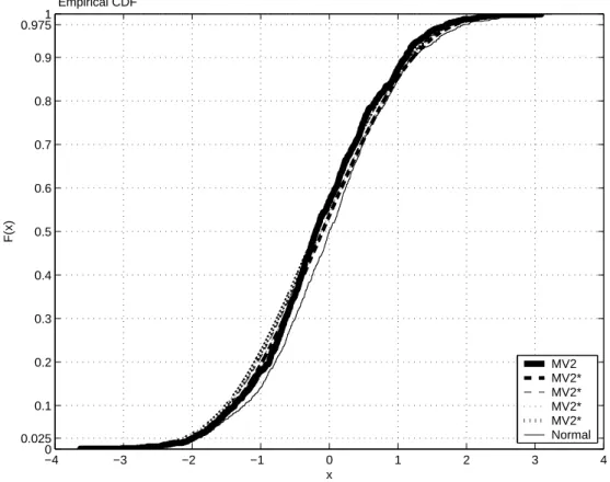
From Figure 3, we can see that the distribution of the MV∗

2 is closer to the CDF of the

sample statistic than the CDF of the standard normal statistic. We expect that the test using bootstrap statistic MV∗

2 will perform better than the traditional test using the standard normal

distribution.

4.2

The size of the tests

Extensive Monte Carlo simulations are conducted to compare the empirical size of different VR tests. The simulation design is as follows. The sample sizes considered are 160, 320, 640 and 1280. For the wild bootstrap test, the number of bootstrap replications m is set to 1000. The holding period k is set to 2,4,8,16,32. The significance level α is 0.05. The test is based on an equal-tailed confidence interval.

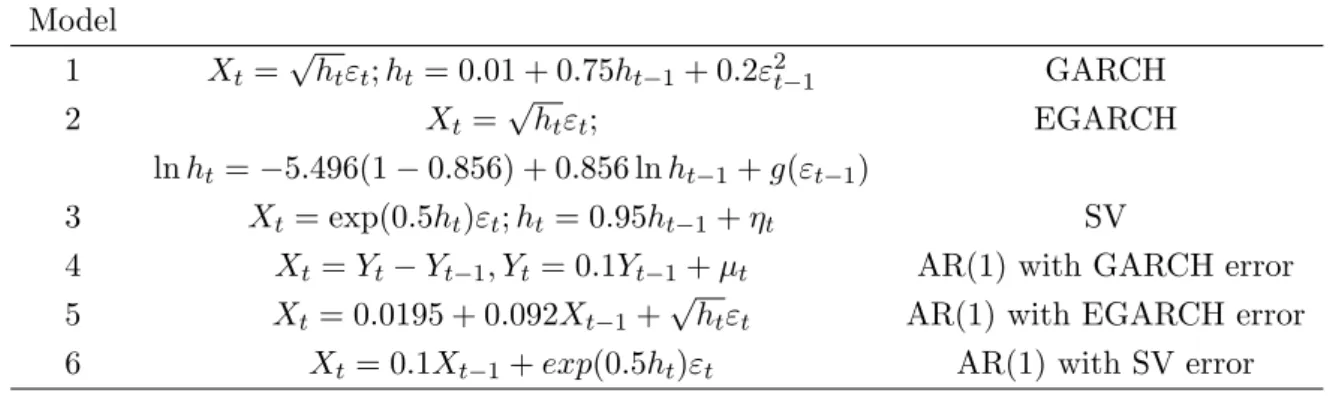
The data generating processes for Xt are simulated, according to the DGP’s list in Table 1.

Table 2 reports the size properties of the asymptotic test using the normal statistic. Table 3 reports the size properties of the wild bootstrap test using MV∗

2. Table 4 reports the size

properties of the wild bootstrap test using MV∗∗

2 , with sample size of 10000 added.

From above tables, we can see that the test with the bootstrap statistic centered at VR suffers from severe size distortions for all sample sizes and k lags considered, even when the sample size is increased to 10000. The size distortions remain big as the number of observations increase, which suggests that the test is not valid asymptotically. As for the test with bootstrap statistic centered at null, there’s no significant size distortion for all the models selected. The test shows desirable size properties even when the holding period k is fairly long.

Table 5 reports the size properties of the wild bootstrap test using MV∗

2 and the test is based

on a symmetric confidence interval.

A comparison of Table 3 and Table 5 shows that the size of the test using symmetric confi-dence interval is similar to that of test using an equal-tailed conficonfi-dence interval. It is not clear whether one outperforms the other.

Interestingly, when we try to compare the size of the test with the bootstrap statistic centered around VR on the basis of symmetric confidence interval, the simulation results report zero size everywhere for all the models and lags considered. To explain this result, we compared the empirical distributions of |MV2| with |MV2∗| and with |MV2∗∗| in Figure 4 and Figure 5,

respectively. The experiment design is similar to the comparison of different distributions at the beginning of Section 3, only we compare here the distributions of the absolute statistics and the VR values chosen are those bigger or equal than three which are extreme values of the distribution |MV2|.

From these figures, we can see that when the bootstrap statistic is centered around VR, the conditional bootstrap distributions of |MV∗∗

|MV2(x; k)|. And the bigger the VR value, the larger the deviation of the conditional bootstrap

distribution from the sample distribution. This observation may help us to understand why we get zero size everywhere when the bootstrap statistic is centered around VR. For example, when the VR value is 3.5447, the estimated quantile of ω1−α/2 we get from the bootstrap distribution

is between 5 and 7, obviously we can’t reject the hypothesis even when the VR value is far away from the null value.

One of possible explanation for the superior performance of the bootstrap statistic centered around 1 may be found in the paper of Li and Maddala (1996). They propose some guidelines of bootstrap testing in the context of linear regression, one of them is to coordinate the re-sampling scheme with the bootstrap statistic. If one re-samples under the null hypothesis, then one should also impose the null hypothesis in the bootstrap statistic by centering it around the null value. In the context of linear regression, we have two options of re-sampling scheme. When constructing the wild bootstrap data, we have choices to impose the null or not to impose the null. However in the VR test case, there’s no choice of re-sampling scheme when applying wild bootstrap. In fact, when we re-sample the sample data by the wild bootstrap, we effectively impose the null, i.e., there is no correlation in the bootstrapped data. Of course, they may still remain the conditional heteroscedasticity. So by the guidelines of Li and Maddala (1996), we need to re-center the bootstrap statistic around the null. The test we proposed here is actually against this principle and as we can see in the simulation experiment, the test suffers a serious size distortion and the result of the test is not reliable. Again, this finding emphasizes the guidelines proposed by Li and Maddala (1996).

4.3

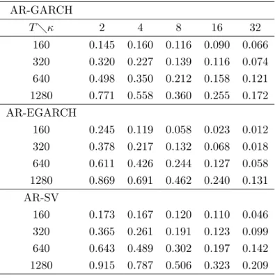
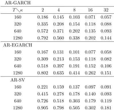
The power of the tests

The power of the asymptotic test is reported in Table 6. Table 7 and Table 8 report the power of the wild bootstrap tests center around 1 based on equal-tailed confidence intervals and symmetric confidence intervals, respectively.

We can see that these tests have similar power. The improvement of the power of the asymptotic test is not significant when using the wild bootstrap statistics centered around 1 in the test, no matter the test are based on equal-tailed confidence intervals or on symmetric confidence intervals.

−4 −3 −2 −1 0 1 2 3 4 0 0.025 0.1 0.2 0.3 0.4 0.5 0.6 0.7 0.8 0.9 0.9751 x F(x) Empirical CDF MV2 MV2** (MV2 = 0,2745) MV2** (MV2 = 0.3767) MV2** (MV2 = −0.8530) MV2** (MV2 = −0.5217) Figure 1: Empirical CDF, MV2 vs MV2∗∗

−4 −3 −2 −1 0 1 2 3 4 0 0.025 0.1 0.2 0.3 0.4 0.5 0.6 0.7 0.8 0.9 0.9751 x F(x) Empirical CDF MV2 MV2* (MV2 = 0.2745) MV2* (MV2 = 0.3767) MV2* (MV2 = −0.8530) MV2* (MV2 = −0.5217) Figure 2: Empirical CDF, MV2 vs MV2∗

−4 −3 −2 −1 0 1 2 3 4 0 0.025 0.1 0.2 0.3 0.4 0.5 0.6 0.7 0.8 0.9 0.9751 x F(x) Empirical CDF MV2 MV2* MV2* MV2* MV2* Normal Figure 3: Empirical CDF, MV∗ 2 vs standard normal

0 0.5 1 1.5 2 2.5 3 3.5 4 0 0.1 0.2 0.3 0.4 0.5 0.6 0.7 0.8 0.9 0.9751 x F(x) Empirical CDF |MV2| |MV2*| (|MV2| = 3.3609) |MV2*| (|MV2| = 3.3122) |MV2*| (|MV2| = 3.5447) |MV2*| (|MV2| = 3.3129) |MV2*| (|MV2| = 3.0892) Figure 4: Empirical CDF, |MV2| vs |MV2∗|

0 1 2 3 4 5 6 7 8 9 10 0 0.1 0.2 0.3 0.4 0.5 0.6 0.7 0.8 0.9 0.9751 x F(x) Empirical CDF |MV2| |MV2**| (|MV2| = 3.3609) |MV2**| (|MV2| = 3.3122) |MV2**| (|MV2| = 3.5447) |MV2**| (|MV2| = 3.3129) |MV2**| (|MV2| = 3.0892) Figure 5: Empirical CDF, |MV2| vs |MV2∗∗|

Table 1: Models used in Monte Carlo experiment Model 1 Xt= √ htεt; ht= 0.01 + 0.75ht−1+ 0.2ε2t−1 GARCH 2 Xt= √ htεt; EGARCH ln ht= −5.496(1 − 0.856) + 0.856 ln ht−1+ g(εt−1) 3 X_t= exp(0.5h_t)ε_t; h_t= 0.95h_t−1+ η_t SV

4 Xt= Yt− Yt−1, Yt= 0.1Yt−1+ µt AR(1) with GARCH error

5 Xt= 0.0195 + 0.092Xt−1+

√

htεt AR(1) with EGARCH error

6 X_t= 0.1X_t−1+ exp(0.5h_t)ε_t AR(1) with SV error

Note:g(εt) = −.0795εt + .2647[|εt| − E(|εt|)]; εt ∼ iidN(0, 1); h0 = 0.01; X0 = 0.01; ηt ∼

iidN(0, 0.1); SV: stochastic volatility; EGARCH model is chosen from Tsay (2002); GARCH

Table 2: Empirical size of asymptotic test, Lo and Mackinlay’s (1988) approach (α = 0.05) GARCH T κ 2 4 8 16 32 160 0.047 0.039 0.041 0.044 0.036 320 0.043 0.043 0.046 0.048 0.041 640 0.057 0.049 0.046 0.045 0.047 1280 0.046 0.048 0.047 0.043 0.052 EGARCH 160 0.044 0.043 0.044 0.038 0.028 320 0.047 0.039 0.047 0.058 0.040 640 0.049 0.050 0.063 0.065 0.047 1280 0.052 0.045 0.058 0.057 0.055 SV 160 0.055 0.047 0.047 0.051 0.025 320 0.058 0.060 0.053 0.044 0.031 640 0.054 0.050 0.050 0.049 0.036 1280 0.061 0.051 0.050 0.051 0.042

Table 3: Empirical size of WB test, center around 1, Kim’s (2006) approach (α = 0.05) GARCH T κ 2 4 8 16 32 160 0.050 0.047 0.050 0.041 0.032 320 0.053 0.033 0.034 0.040 0.049 640 0.051 0.054 0.050 0.047 0.059 1280 0.060 0.046 0.051 0.053 0.044 EGARCH 160 0.052 0.058 0.050 0.039 0.044 320 0.052 0.041 0.043 0.039 0.053 640 0.070 0.058 0.049 0.055 0.058 1280 0.059 0.044 0.064 0.065 0.054 SV 160 0.050 0.049 0.051 0.057 0.050 320 0.056 0.052 0.058 0.045 0.048 640 0.058 0.056 0.048 0.049 0.034 1280 0.054 0.049 0.044 0.047 0.046

Table 4: Empirical size of WB test, center around VR (α = 0.05) GARCH T κ 2 4 8 16 32 160 0.458 0.432 0.446 0.537 0.638 320 0.437 0.416 0.394 0.401 0.460 640 0.418 0.396 0.386 0.419 0.454 1280 0.453 0.424 0.417 0.379 0.401 10000 0.436 0.436 0.397 0.407 0.394 EGARCH 160 0.414 0.437 0.444 0.548 0.638 320 0.411 0.426 0.410 0.431 0.460 640 0.417 0.385 0.426 0.455 0.454 1280 0.413 0.386 0.369 0.396 0.401 10000 0.402 0.391 0.421 0.473 0.396 SV 160 0.454 0.462 0.470 0.525 0.638 320 0.402 0.393 0.397 0.410 0.465 640 0.394 0.396 0.424 0.415 0.409 1280 0.415 0.363 0.359 0.365 0.376 10000 0.385 0.364 0.447 0.403 0.359

Table 5: Empirical size of WB test, center around 1, based on symmetric confidence intervals (α = 0.05) GARCH T κ 2 4 8 16 32 160 0.058 0.055 0.044 0.045 0.031 320 0.049 0.046 0.059 0.055 0.056 640 0.044 0.063 0.037 0.054 0.051 1280 0.062 0.052 0.074 0.061 0.053 EGARCH 160 0.056 0.046 0.050 0.041 0.038 320 0.053 0.055 0.068 0.052 0.049 640 0.054 0.059 0.039 0.053 0.055 1280 0.057 0.066 0.069 0.060 0.058 SV 160 0.048 0.039 0.052 0.053 0.056 320 0.060 0.070 0.049 0.050 0.044 640 0.058 0.042 0.064 0.061 0.060 1280 0.066 0.054 0.044 0.049 0.045

Table 6: Power of the asymptotic test

AR-GARCH T κ 2 4 8 16 32 160 0.145 0.160 0.116 0.090 0.066 320 0.320 0.227 0.139 0.116 0.074 640 0.498 0.350 0.212 0.158 0.121 1280 0.771 0.558 0.360 0.255 0.172 AR-EGARCH 160 0.245 0.119 0.058 0.023 0.012 320 0.378 0.217 0.132 0.068 0.018 640 0.611 0.426 0.244 0.127 0.058 1280 0.869 0.691 0.462 0.240 0.131 AR-SV 160 0.173 0.167 0.120 0.110 0.046 320 0.365 0.261 0.191 0.123 0.099 640 0.643 0.489 0.302 0.197 0.142 1280 0.915 0.787 0.506 0.323 0.209

Table 7: Power of the WB test, based on equal-tailed confidence intervals AR-GARCH T κ 2 4 8 16 32 160 0.186 0.145 0.103 0.071 0.057 320 0.335 0.208 0.154 0.118 0.088 640 0.572 0.371 0.202 0.135 0.093 1280 0.792 0.560 0.338 0.202 0.144 AR-EGARCH 160 0.167 0.131 0.101 0.077 0.058 320 0.309 0.213 0.153 0.118 0.082 640 0.518 0.397 0.191 0.152 0.106 1280 0.802 0.635 0.414 0.262 0.151 AR-SV 160 0.221 0.159 0.137 0.097 0.091 320 0.415 0.278 0.178 0.140 0.093 640 0.726 0.518 0.303 0.179 0.119 1280 0.905 0.798 0.505 0.302 0.181

Table 8: Power of the WB test, based on symmetric confidence intervals

AR-GARCH T κ 2 4 8 16 32 160 0.108 0.119 0.101 0.075 0.062 320 0.248 0.189 0.156 0.127 0.087 640 0.479 0.381 0.197 0.159 0.120 1280 0.769 0.624 0.427 0.266 0.163 AR-EGARCH 160 0.241 0.123 0.078 0.040 0.032 320 0.356 0.264 0.152 0.085 0.065 640 0.598 0.421 0.228 0.132 0.081 1280 0.864 0.687 0.449 0.270 0.138 AR-SV 160 0.164 0.151 0.142 0.101 0.100 320 0.362 0.264 0.192 0.155 0.113 640 0.689 0.511 0.314 0.189 0.138 1280 0.899 0.790 0.510 0.319 0.201

5

Conclusion

The variance ratio test has been widely used as a means of testing for the martingale hypothesis in financial time series. The conventional VR tests are based on asymptotic approximations, which may not be reliable when the sample size is not large enough to justify the asymptotic theories involved. These small sample deficiencies can lead to misleading inferential outcomes in practical applications. Kim (2006) uses the wild bootstrap in the VR test and shows that this method has desirable size properties under a wide range of data generation processes. Kim’s method uses bootstrap statistic centered around the null hypothesis. In this paper, we propose a VR test based on the wild bootstrap in which the bootstrap statistic is centered around sample statistic.

Extensive Monte Carlo simulations are conducted to compare size and power properties of the wild bootstrap tests. It is found that the distribution of the bootstrap statistic centered at sample statistic is not stable and suffers severe distortions from the distribution of the sample statistic. When the test is based on an equal-tailed confidence interval, the test using the bootstrap statistic centered around the sample statistic shows large possibility of rejection compared to the nominal rejection level. When the test is based on a symmetric confidence interval, the size is zero everywhere for all the models and lags considered. As a result, the size of the test is largely distorted and make this test not reliable. By contrast, the test using the bootstrap statistic centered around the null hypothesis shows desirable size and power properties.

From this finding, we emphasize the guidelines proposed by Li and Maddala (1996) that coordinating the bootstrap sample scheme with the bootstrap centering is important for good finite sample results. In particular, the paper has shown that if one re-samples under the null hypothesis, then one should also impose the null hypothesis in the bootstrap statistic by centering it around the null value. Although the discussion of Li and Maddala (1996) is limited to the linear regression, the principle applies also to the VR test. In fact, when applying the wild bootstrap to the VR test, we are effectively bootstrapping under the null hypothesis being tested, so the only appropriate bootstrap statistic is the one centered by the null value.

References

Ayadi, O. F., Pyun, C. S., 1994. An application of variance ratio test to the korean securities market. Journal of Banking and Finance 18, 643-658.

Fong, W. M., Koh, S. K., Ouliaris, S., 1997. Joint variance-ratio tests of the martingale hypothesis for exchange rates. Journal of Business and Economic Statistics 15, 51-59.

Goncalves, S. , Kilian, L., 2004. Bootstrapping autoregressions with conditional heteroskedas-ticity of unknown form. Journal of Econometrics 123, 89-120.

Hall, P., 1992. The Bootstrap and Edgeworth Expansion. Springer, New York.

Li, H., Maddala, G.S., 1996. Bootstrapping time series models. Econometric reviews 15, 115-158.

Kim, J. H., 2006. Wild bootstrapping variance ratio tests. Economics Letters 92, 38-43. Liu, C. Y. , He, J., 1991. A variance-ratio test of random-walks in foreign-exchange rates. Journal of Finance 46, 773-785.

Lo, A. W. , Mackinlay, A. C., 1989. The size and power of the variance ratio test in finite samples - a monte-carlo investigation. Journal of Econometrics 40, 203-238.

Lo, A. W. , Mackinlay, A.C., 1988. Stock market prices do not follow random walks: Evidence form a simple specification test. The Review of Financial Studies 1, 41-66.

Malliaropulos, D., R Priestley, 1999. Mean reversion in southeast asian stock markets. Journal of Empirical Finance 6, 355-384.

Mammen, E., 1993. Bootstrap and wild bootstrap for high-dimensional linear-models. The annals of statistics 21, 255-285.

Richardson, M., 1989. Drawing inferences from statistics based on multiyear asset returns. Journal of financial economics 25, 323-348.

Tsay, R.S., 2002. Analysis of Financial Time Series. Wiley, New York.

van Giersbergen, N. P. A., 2002. How to implement the bootstrap in static or stable dynamic regression models: test statistic versus confidence region approach. Journal of econometrics 108, 133-156. 0304-4076.

Wu, C. F. J., 1986. Jackknife, bootstrap and other resampling methods in regression-analysis - discussion. Annals of Statistics 14, 1261-1295.

Yilmaz, K., 2003. Martingale property of exchange rates and central bank interventionssd. Journal of Business and Economic Statistics 21, 383-395.