Training Deep Convolutional Architectures for Vision
par
Guillaume Desjardins
Département d’informatique et de recherche opérationnelle Faculté des arts et des sciences
Mémoire présenté à la Faculté des arts et des sciences en vue de l’obtention du grade de Maître ès sciences (M.Sc.)
en informatique
Août, 2009
c
Faculté des arts et des sciences
Ce mémoire intitulé:
Training Deep Convolutional Architectures for Vision
présenté par: Guillaume Desjardins
a été évalué par un jury composé des personnes suivantes:
Pascal Vincent président-rapporteur Yoshua Bengio directeur de recherche Sébastien Roy membre du jury
Les tâches de vision artificielle telles que la reconnaissance d’objets demeurent irréso-lues à ce jour. Les algorithmes d’apprentissage tels que les Réseaux de Neurones Artifi-ciels (RNA), représentent une approche prometteuse permettant d’apprendre des carac-téristiques utiles pour ces tâches. Ce processus d’optimisation est néanmoins difficile. Les réseaux profonds à base de Machine de Boltzmann Restreintes (RBM) ont récem-ment été proposés afin de guider l’extraction de représentations intermédiaires, grâce à un algorithme d’apprentissage non-supervisé. Ce mémoire présente, par l’entremise de trois articles, des contributions à ce domaine de recherche.
Le premier article traite de la RBM convolutionelle. L’usage de champs réceptifs locaux ainsi que le regroupement d’unités cachées en couches partageant les même pa-ramètres, réduit considérablement le nombre de paramètres à apprendre et engendre des détecteurs de caractéristiques locaux et équivariant aux translations. Ceci mène à des modèles ayant une meilleure vraisemblance, comparativement aux RBMs entraînées sur des segments d’images.
Le deuxième article est motivé par des découvertes récentes en neurosciences. Il analyse l’impact d’unités quadratiques sur des tâches de classification visuelles, ainsi que celui d’une nouvelle fonction d’activation. Nous observons que les RNAs à base d’unités quadratiques utilisant la fonction softsign, donnent de meilleures performances de généralisation.
Le dernière article quand à lui, offre une vision critique des algorithmes populaires d’entraînement de RBMs. Nous montrons que l’algorithme de Divergence Contrastive (CD) et la CD Persistente ne sont pas robustes : tous deux nécessitent une surface d’éner-gie relativement plate afin que leur chaîne négative puisse mixer. La PCD à "poids ra-pides" contourne ce problème en perturbant légèrement le modèle, cependant, ceci gé-nère des échantillons bruités. L’usage de chaînes tempérées dans la phase négative est une façon robuste d’adresser ces problèmes et mène à de meilleurs modèles génératifs.
Mots clés: réseau de neurone, apprentissage profond, apprentissage non-supervisé, apprentissage supervisé, RBM, modèle à base d’énergie, tempered MCMC
High-level vision tasks such as generic object recognition remain out of reach for mod-ern Artificial Intelligence systems. A promising approach involves learning algorithms, such as the Arficial Neural Network (ANN), which automatically learn to extract useful features for the task at hand. For ANNs, this represents a difficult optimization problem however. Deep Belief Networks have thus been proposed as a way to guide the discov-ery of intermediate representations, through a greedy unsupervised training of stacked Restricted Boltzmann Machines (RBM). The articles presented here-in represent contri-butions to this field of research.
The first article introduces the convolutional RBM. By mimicking local receptive fields and tying the parameters of hidden units within the same feature map, we con-siderably reduce the number of parameters to learn and enforce local, shift-equivariant feature detectors. This translates to better likelihood scores, compared to RBMs trained on small image patches.
In the second article, recent discoveries in neuroscience motivate an investigation into the impact of higher-order units on visual classification, along with the evaluation of a novel activation function. We show that ANNs with quadratic units using the softsign activation function offer better generalization error across several tasks.
Finally, the third article gives a critical look at recently proposed RBM training al-gorithms. We show that Contrastive Divergence (CD) and Persistent CD are brittle in that they require the energy landscape to be smooth in order for their negative chain to mix well. PCD with fast-weights addresses the issue by performing small model pertur-bations, but may result in spurious samples. We propose using simulated tempering to draw negative samples. This leads to better generative models and increased robustness to various hyperparameters.
Keywords: neural network, deep learning, unsupervised learning, supervised learning, RBM, energy-based model, tempered MCMC
RÉSUMÉ . . . iii ABSTRACT . . . iv CONTENTS . . . v LIST OF TABLES . . . ix LIST OF FIGURES . . . x LIST OF APPENDICES . . . xi
LIST OF ABBREVIATIONS . . . xii
NOTATION . . . xiii
DEDICATION . . . xv
ACKNOWLEDGMENTS . . . xvi
CHAPTER 1: INTRODUCTION . . . 1
1.1 Introduction to Machine Learning . . . 2
1.1.1 What is Machine Learning . . . 2
1.1.2 Empirical Risk Minimization . . . 4
1.1.3 Parametric vs. Non-Parametric . . . 5
1.1.4 Gradient Descent: a Generic Learning Algorithm . . . 8
1.1.5 Overfitting, Regularization and Model Selection . . . 9
1.2 Logistic Regression: a Probabilistic Linear Classifier . . . 10
1.3 Artificial Neural Networks . . . 13
1.3.1 Architecture . . . 13
1.3.3 Implementation Details . . . 17
1.3.4 Challenges . . . 18
1.4 Convolutional Networks . . . 20
1.5 Alternative Models of Computation . . . 22
CHAPTER 2: DEEP LEARNING . . . 24
2.1 Boltzmann Machine . . . 25
2.2 Markov Chains and Gibbs Sampling . . . 27
2.2.1 Markov Chains . . . 27
2.2.2 The Gibbs Sampler . . . 28
2.3 Deep Belief Networks . . . 29
2.3.1 Restricted Boltzmann Machine . . . 29
2.3.2 Contrastive Divergence . . . 31
2.3.3 Greedy Layer-Wise Training . . . 32
CHAPTER 3: OVERVIEW OF THE FIRST PAPER . . . 34
3.1 Context . . . 34
3.2 Contributions . . . 34
3.3 Comments . . . 35
CHAPTER 4: EMPIRICAL EVALUATION OF CONVOLUTIONAL RBMS FOR VISION . . . 36
4.1 Abstract . . . 36
4.2 Introduction . . . 36
4.3 Restricted Boltzmann Machines . . . 37
4.4 Convolutional RBMs . . . 39
4.4.1 Architecture of CRBMs . . . 39
4.4.2 Contrastive Divergence for CRBMs . . . 41
4.5 Experiments . . . 42
4.6 Results and Discussion . . . 44
4.8 Conclusion . . . 46
CHAPTER 5: OVERVIEW OF THE SECOND PAPER . . . 49
5.1 Context . . . 49
5.2 Contributions . . . 49
5.3 Comments . . . 50
CHAPTER 6: QUADRATIC POLYNOMIALS LEARN BETTER IMAGE FEATURES . . . 51
6.1 Abstract . . . 51
6.2 Introduction . . . 51
6.3 Model and Variations . . . 55
6.3.1 Learning . . . 56
6.3.2 Sparse Structure and Convolutional Structure . . . 57
6.3.3 Support Vector Machines . . . 59
6.4 Data Sets . . . 59 6.4.1 Shape Classification . . . 59 6.4.2 Flickr . . . 60 6.4.3 Digit Classification . . . 61 6.5 Results . . . 61 6.5.1 Translation Invariance . . . 62 6.5.2 Tanh vs. Softsign . . . 63 6.6 Discussion . . . 64
CHAPTER 7: OVERVIEW OF THE THIRD PAPER . . . 67
7.1 Context . . . 67
7.2 Contributions . . . 68
7.3 Comments . . . 69
CHAPTER 8: TEMPERED MARKOV CHAIN MONTE CARLO FOR
. . . 70
8.1 Abstract . . . 70
8.2 Introduction and Motivation . . . 70
8.3 RBM Log-Likelihood Gradient and Contrastive Divergence . . . 72
8.4 Tempered MCMC . . . 73
8.5 Experimental Observations . . . 75
8.5.1 CD-k: local learning ? . . . 75
8.5.2 Limitations of PCD . . . 77
8.5.3 Tempered MCMC for training and sampling RBMs . . . 78
8.5.4 Tempered MCMC vs. CD and PCD . . . 79
8.5.5 Estimating Likelihood on MNIST . . . 81
8.6 Conclusion . . . 83
CHAPTER 9: CONCLUSION . . . 85
9.1 Article Summaries and Discussion . . . 85
9.1.1 Empirical Evaluation of Convolutional Architectures for Vision 85 9.1.2 Quadratic Polynomials Learn Better Image Features . . . 86
9.1.3 Tempered Markov Chain Monte Carlo for Training of Restricted Boltzmann Machines . . . 87
9.1.4 Discussion . . . 87
9.2 Future Directions . . . 88
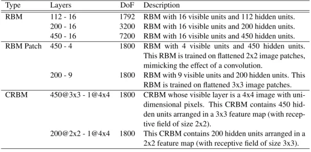
4.1 Overview of CRBM Architectures Tested . . . 45
6.1 Generalization Error . . . 62
6.2 Results on Translation Invariance . . . 63
6.3 Generalization Error: tanh vs. softsign . . . 64
1.1 Linear Classifier . . . 11
1.2 Sigmoid Function and Logistic Regression . . . 13
1.3 Graphical Representation of Logistic Regression and a Multi-Layer Per-ceptron . . . 14
1.4 Convolutional Neural Network . . . 21
2.1 Boltzmann Machine and Restricted Boltzmann Machine . . . 30
2.2 Deep Belief Network . . . 32
4.1 Contrastive Divergence in convolutional RBMs . . . 41
4.2 Example Training Data . . . 43
4.3 Performance of RBM (dense, patch) vs. CRBMs . . . 47
6.1 Sigmoid vs. Softsign . . . 54
6.2 Architecture of Sparse and Convolutional Quadratic Networks . . . 58
6.3 Samples from MNIST, Shapeset and Flickr Datasets . . . 60
8.1 Samples Obtained with CD . . . 76
8.2 Samples Obtained with PCD . . . 78
8.3 Samples Obtained with PCD with fast weights . . . 78
8.4 Samples Obtained with PCD . . . 79
2D Two Dimensional AI Artificial Intelligence ANN Artificial Neural Network
BM Boltzmann Machine CD Contrastive Divergence CNN Convolutional Neural Network
CPU Central Processing Unit
CRBM Convolutional Restricted Boltzmann Machine DBN Deep Belief Network
FPCD Persistent Contrastive Divergence with fast-weights HOTLU Higher-Order Threshold Logic Unit
I.I.D Independent and Identically-Distributed MCMC Markov Chain Monte Carlo
ML Machine Learning MLP Multi-Layer Perceptron MSE Mean-Squared Error
NLL Negative Log-Likelihood
PCD Persistent Contrastive Divergence RBF Radial Basis Function
RBM Restricted Boltzmann Machine SIFT Scale Invariant Feature Transform SVM Support Vector Machines
D Dataset containing training examples and possibly labels/targets Dvalid Dataset containing examples /∈ D: used to choose optimal
hyperparam-etersθH
Dtest Dataset containing examples /∈ D,Dvalid: used to estimate
generaliza-tion error
dh number of neurons in hidden layer
Ep(x) Expectation with regards to probability density p(x) f Prediction function
fθ Function f parametrized by parametersθ
g(x) discriminant function
h(a),h vector of hidden units in MLP, before and after activation function Ix indicator function (1 if x is true, 0 otherwise)
K(x,y) Kernel function applied to points x and y
KL(p1,p2) KL-divergence of probability densities p1and p2
L Loss function used during minimization Lβ size of mini-batch
m Label predicted by prediction function f
Nµ,σ Gaussian probability distribution with meanµ and covariance σ
o(a),o vector of output units in MLP, before and after activation function p(x) Model estimate of the true empirical distribution pT(x)
p(x,y) Model estimate of the true joint-probability density function pT(x,y)
p(y|x) Model estimate of the true conditional probability density function pT(y|x)
φ Non-linear function
R( f , D) Empirical risk of prediction function f measured over dataset D Rd Set of all real numbers with dimensionality d
s (non-linear) squashing function θ Set of parameters to learn θH Set of all hyperparameters
W upper-case indicates a matrix, unless specified otherwise w lower-case indicates a vector, unless specified otherwise WT transpose of matrix or vector
Wi· i-th row of matrix W W· j j-th column of matrix W
Wi j element in i-th row and j-th column of matrix W
wi i-th element of vector w
x(i) i-th training example, x(i)∈ Rd
x ∼ p(x) x is a sample drawn from probability density p(x) y(i) Label or target for i-th training example
z(i) In supervised learning, (x(i),y(i)), in unsupervised learning (x(i)) Z Normalization constant
(c,V,b,W) parameters of MLP: offset vector c and weight matrix V of hidden layer; offset vector b and weight matrix W of output layer
∂ f ∂x
� �
First and foremost, I would like to thank Yoshua Bengio for taking me under his wing and giving me the tools to one-day (hopefully) succeed in research. His vast knowledge of machine learning is only trumped by his passion for research and understanding, a trait which is often contagious. By fostering creativity, independent thinking and open discussions, Yoshua has created a truly motivating and rewarding atmosphere within the lab, in which it is a pleasure to be a part of. I would also like to thank Aaron Courville for many thought provoking (and sometimes long) discussions, which have helped mold my current understanding of machine learning. Special thanks also go to James Bergstra and Olivier Breuleux not only for their work on Theano, but also for always making themselves available to help. Along the same lines, thanks to Frédéric Bastien, who despite being pulled in many directions, always finds time to help out.
Last but not least, thank you to my friends and family for their encouragements. Madeleine, thank you for putting up with the late hours, the ups and downs of research and for always being there for me (even when far away). This would not have been possible without you.
INTRODUCTION
It is reported that Marvin Minsky, one of the founding fathers of Artificial Intelligence (AI), once assigned as a summer project, the task of building an artificial vision system capable of describing what it saw. Several decades later, visual object recognition still remains a largely unsolved problem. At the time of this writing, state-of-the-art results on Caltech 101 (a benchmark dataset containing objects of 101 categories to identify in natural images) hover around 65% accuracy [31]. So what makes object recognition and artificial perception so difficult ?
Real-world images are the result of complex interactions between lighting, scene geometry, textures and an observer (i.e. the human eye or a camera). Small variations at any stage of this image formation process can have profound effects on the resulting 2D image. For example, two identical pictures taken at different times of day may look more dissimilar (in terms of average euclidean distance between pixels) than pictures of different scenes taken in the same lighting conditions. Changes in viewpoint can also contribute to making a single object unrecognizable once rotated, if using a simple template matching approach1. The difficulty of generic object recognition is further
compounded by the fact that two objects belonging to the same object category, may be more visually dissimilar, than objects of a competing class. Building a robust computer vision system therefore involves building a system which is invariant to many (if not all) of the afore-mentioned sources of variation.
Object recognition systems often use a two-stage pipeline to solve this problem. The first stage involves extracting a set of features from the input data, which is then used as input to a classification module. These features are often hand-crafted to be invariant to certain forms of variations. For example, SIFT features [43] have been shown to be robust to scale, lighting and small amounts of rotation. While these features are still
1Template matching consists in convolving the input with a prototypical image of the object of interest
competitive on Caltech-101, their development requires extensive engineering. Also, it is not clear how one would engineer features to be robust across higher-level abstractions ("animal species" for example). It would be ideal if such features could be automatically learnt from training data. This would allow features to be tuned automatically in order to maximize the performance of the system, while also requiring the development of a single algorithm which would work across many settings. To this end, we turn to the field of Machine Learning, which has shown, since the inception of the Artificial Neural Network, that this is indeed an achievable goal.
In this chapter, we start by giving a brief overview of Machine Learning and explain the core principles behind the most common learning algorithms. In section 1.3, we explain in detail the Artificial Neural Network (ANN) and show how it can automatically perform feature extraction and classification. Sections 1.4 and 1.5 explore biologically motivated variants of ANNs which will be the focus of later chapters. We then build on this knowledge and explore in Chapter 2, recent developments in the field of neural network research : the Deep Belief Network, which embodies the principles of Deep Learning. Chapters 3-8 represent the core of this thesis and consist of three articles pertaining to the field of deep networks and ANNs applied to vision.
1.1 Introduction to Machine Learning 1.1.1 What is Machine Learning
Machine Learning (ML) is a sub-field of AI, which focuses on the statistical nature of learning. The goal of ML is to develop algorithms which learn directly from data by exploiting the statistical regularities present in the signal. Intelligence or intelligent behaviour, is thus regarded as the ability to apply this knowledge to novel situations. This concept is known asgeneralization. A learning algorithm can thus be described as any algorithm which takes as input atraining set D and outputs a model or prediction function f. The quality of this learnt model is then determined by the accuracy of the prediction on a separate hold-out dataset known as thetest set Dtest. A model which
The exact nature of the datasets varies depending on the intended applications. In the context of supervised learning, the goal is to learn a mapping between a series of observa-tions and associated targets. The training set can be written as D = {(x(i),y(i));i = 1..n} where x(i)∈ Rd is an input datum with target y(i). We will define z(i)as being the pair
(x(i),y(i)) and consider z(i) to be independent and identically distributed (IID) samples
from the true underlying distribution pT(z). The target y(i) may be discrete or
contin-uous. The discrete case corresponds to aclassification task, where y(i) ∈ {1,...,m} is
one of m possiblecategories or labels to assign to input x(i). In object recognition, the x(i)’s would correspond to the input images and the y(i)’s to a numerical value indi-cating the type of object present within the image. From a probabilistic point of view, the general concept is to learn an estimate p(y|x) of pT(y|x) directly from the training
data {(x(i),y(i))}. p(y|x) is vector-valued and contains the class membership
probabili-ties p(yj|x), j ∈ {1,...,m} for all possible classes of input x. The predicted class is then
given by f (x) = argmaxjp(yj|x). The resulting module is called a classifier and is a
central building block of many object recognition systems. If the target y is continuous-valued, the problem is one ofregression. The goal is then to generate an output so as to match a given statistic of pT(y|x), for example EpT(x,y)(Y |X). Predicting the
posi-tion of the object within the input images (as opposed to the nature of the object) would constitute a regression task.
When no target y is given, learning is said to be unsupervised and z(i)= x(i). The
learner then simply tries to model the input distribution pT(x), or aspects thereof.
Prob-abilistic modeling of pT(y|x) is often referred to as density estimation, which strictly
speaking, assumes that x is continuous-valued. Unsupervised learning is often used for exploratory data analysis, in order to gain a better understanding of the data. Algorithms such as k-means or mixtures of Gaussians for example, can be used to extract the most salient modes of a distribution and help to extract natural groupings within the data, a task known asclustering. One can also augment the model p(x) by adding hidden or latent variables h to the model. p(x) can then be rewritten as p(x) = ∑hp(x,h). The
state of the hidden units being unknown, they must therefore be inferred by finding the most probable values for h. This task is known asinference and can be used to find "root
causes" or "explanations" for the visible data. As we will see later on in section 2.3.1, the Restricted Boltzmann Machine (RBM) works along this principle and is used to extract useful features from the data. Unsupervised learning can also be used to build gener-ative models, where the trained system can output samples ˜x ∼ p(x) which mimic the training distribution. A hybrid method also consists in using unsupervised learning to learn a model p(x,y) of the joint distribution, which in turn can be used for classification. Other variants of ML include semi-supervised learning where D consists of both labeled and unlabeled examples. Reinforcement learning deals with the problem of de-layed reward, where the supervised signal (or reinforcement) is provided only after a series of actions have been taken and depends on the actions taken along the way. We are intentionally leaving out discussion of these sub-fields of ML as they are not directly relevant to the contents of this thesis.
1.1.2 Empirical Risk Minimization
While we have given a general definition of what a learning algorithm should look like, we still have not specified how the actual learning occurs. How do we actually obtain this function f from D ? Most ML algorithms utilize theempirical risk mini-mization strategy.
Given aloss function L and a dataset D, the empirical risk is defined as:
R( f , D) = 1/n
n
∑
i=1
L (x(i),y(i); f ) (1.1)
Learning consists in finding the function or model f which minimizes the average loss across the training set. Learning should therefore return the function f such that:
f ← argminf∗R( f∗, D)
This recipe for learning is problematic however. Indeed, there is an easy and trivial solution to this minimization process. The model can simply learn the training set by heart (i.e. by making a copy of the data in memory) and for each x(i)output the associated
y(i). Such a model would obtain the lowest value for R. It would be absurd however,
to claim that such a system has learnt anything useful about the data or to relate this model to "intelligent behaviour" of any kind. As mentioned previously, what we are ultimately interested in is the generalization capability of our model. To evaluate the true performance of a model, we therefore use R( f ,Dtest), the average risk across test
set Dtest= {zi;zi�∈ D}.
The choice of loss function will vary depending on the application. Generally speak-ing however, the followspeak-ing loss functions are used:
• Classification: classification error. Lclassi f .(x(i),y(i); f ) =If (x(i))!=y(i), i.e. a unity
loss whenever the predicted class label is not the correct one. For reasons we will explore in section 1.1.4, it can be advantageous for the loss function to be continuous and differentiable. In that case, probabilistic classifiers may use the conditional likelihood loss (section 1.2).
• Regression: mean-squared error loss. LMSE(x(i),y(i); f ) = ( f (x(i)) − y(i))2. The
empirical risk will thus be the average squared error between predicted values and the real targets.
• Density Estimation: negative-likelihood loss. LNLL(x(i); f ) = −log f (x(i)), where
f (x) is the estimate p(x) of the underlying distribution pT(x). In the case of
para-metric models indexed by parametersθ (section 1.1.3), this leads to the solution which maximizes p(D|θ), an instance of the maximum likelihood solution.
1.1.3 Parametric vs. Non-Parametric
Machine learning algorithms can generally be split into two families: parametric and non-parametric methods.
Parametric algorithms are those which model a particular probability distribution, using a fixed set of parametersθ. The function or model is written as fθ. In this setting,
learning amounts to finding the optimal parametersθ so as to minimize R( fθ, D). The
well one can approximate the distribution of interest. A typical parametric method for density estimation is the mixture of Gaussians model, which estimates p(x) as the sum of multiple Gaussian probability distributions such that p(x) =∑Kk=1πkN (x|µk,Σk), where
N (x|µk,Σk) is a Gaussian distribution with meanµkand covariance matrixΣk. K is the
total number of Gaussians used by the model and πk is the weight associated to each
Gaussian (with the constraint∑Kk=1πk= 1). The optimal parametersθ = {(µk,Σk,πk),k =
1..K} can be determined through maximum likelihood by solving ∂R/∂θ = 0. The main drawback of parametric methods is the constraints imposed by the choice of a fixed model. Choosing an improper model (e.g. a single Gaussian to model a multi-modal dis-tribution) can result in poor performance. Parametric models of relevance to this thesis include logistic regression (section 1.2), artificial neural networks (section 1.3) and Deep Belief Networks (DBN) (section 2.3).
Non-parametric methods are more flexible in that they make no inherent assump-tions about the distribuassump-tions to model. A large family of non-parametric algorithms use the training data itself to model the distribution. The most basic non-parametric algo-rithm is the well-known histogram method. For input data x(i)∈ Rd, the input data space
is divided into kd equally-sized bins. The probability density can then be estimated lo-cally, within each bin as
pi=n∆ni i,
where ni is the number of data points falling within bin-i, n the total number of points
in D and ∆i the width of the bin. Parzen Windows is another hallmark non-parametric
density estimation method which greatly improves on the histogram method. Instead of partitioning the space into equally sized bins and assigning probability mass in a discrete manner, each data point x(i)∈ D contributes an amount 1/nK(x(i),x) to p(x), where K(x(i),x) is a smooth kernel centered on x(i). The density estimate is therefore: p(x) = 1/n∑n
i=1K(x(i),x), A popular choice for K is the multi-variate Gaussian density
function with meanµ = x(i). The varianceσ2 of this Gaussian kernel is referred to as a
hyperparameter (and not a parameter) since it cannot be learnt by maximum likelihood on the training data. Indeed, learning the variance by minimizing R would result in a
null variance, possibly leading to an infinite loss on the test set. In the future, we will denote the set of hyperparameters required by a model f asθH. We will see later on in
Chapter 8, a real-world usage scenario of how Parzen Windows can be used to estimate the density p(x) defined by a Restricted Boltzmann Machine.
Parametric algorithms may also contain hyperparameters. Typical examples include learning rates (section 1.1.4), stopping criteria (sections 1.1.4, 1.1.5) and regulariza-tion constants (secregulariza-tion 1.1.5). In practice, the distincregulariza-tion between parametric and non-parametric methods is also often blurry. For example, Artificial Neural Networks (ANN), Deep Belief Networks (DBN) and mixture models can be considered non-parametric if the number of hidden units or components in the mixture is parameterizable. A method for choosing good hyperparameter values is covered in section 1.1.5.
Many non-parametric methods are said to belocal methods. This is the case when their prediction for test point x( j) depends on training data at a relatively short distance from x( j) (whether for classification, regression or density estimation). Local methods are thus much more prone to thecurse of dimensionality, which states that the amount of data (cardinality of D) required to span an input space Rdis exponential in the number
of dimensions d. As such, the performance of these algorithms degrades significantly for higher values of d, unless compensated by an exponential increase in training data.
For vision applications, we are usually dealing with inputs of very large dimension-ality. In the simplest case of hand-written digit recognition, such as the MNIST dataset [39], input images are of size 28x28 pixels and can easily scale up to hundreds of thou-sands of pixels for more complicated datasets. While the true dimensionality of the data (i.e the dimension of the manifold on which the training distribution is concentrated) is usually unknown and no doubt smaller than the raw number of pixels, the inherent com-plexity of vision problems suggests that this phenomenon is definitely at play. For this reason, this thesis will focus onglobal methods, which are not as prone to the curse of dimensionality and are much better suited to the problem at hand.
1.1.4 Gradient Descent: a Generic Learning Algorithm
Gradient Descent is a well-known first-order optimization technique for finding a minimum of a given function. For any multivariate function f (x) (with x = [x1, ...,xd])
differentiable at point a, the direction of steepest ascent is given by the vector of partial derivatives, [∂x∂ f 1 � � �x=a, ...,∂x∂ f d � �
�x=a] at point a. If we initialize x0 = a and ||∂ f (a)∂x || > 0,
performing an infinitesimal step in the opposite direction of this gradient is guaranteed to achieve a lower value for f (x). This suggests the iterative algorithm of Algorithm 1 for minimizing the empirical risk R.
Algorithm 1 BatchGradDescentLearning(L , fθ, D, ε)
L: loss function to minimize across training set D fθ: prediction function parameterized by parametersθ
D: dataset of training examples
ε: learning rate or step-size for gradient descent Initialize model parameters of fθ to ˜θ
while stopping condition is not met do Initialize ∂R∂θ to 0
for all z(i)∈ D do ∂R ∂θ ←∂R∂θ +∂L (z (i),fθ) ∂θ |θ= ˜θ end for ˜θ ← ˜θ −ε∂R ∂θ
Update model parameters of fθto ˜θ
end while return fθ
The above procedure is known as abatch learning method, since it requires a com-plete pass through the training set D before performing a parameter update. In practice, this procedure is guaranteed to converge as long as certain conditions on the learning rate are satisfied2. Furthermore, if the loss function is convex in θ, it will converge to the
global minimum. Gradient descent of non-convex functions may lead to local minima however.
An alternative learning algorithm, known asstochastic gradient descent has proven
2To guarantee convergence,ε
t must actually have a decreasing profile as a function of t, such that
very efficient in practice [39]. The trick is to get rid of the inner-most loop and update the parameters for each training example z(i). While this update does not follow the exact gradient of R( f ,D), the redundancy in the training data (examples are IID) tends to make this algorithm converge much faster. The randomness introduced by the stochastic updates has also been shown to help with escaping from local minima. A hybrid method also exists, namedstochastic gradient with mini-batches, which consists in updating the parameters every Lβ training examples, where Lβ is usually in the range 1 < Lβ <
100. This has several advantages, the first of which is to help reduce the variance of the gradient updates.3
How to initialize the parameters and when to stop the gradient descent procedure usually vary based on the application. In section 1.3, we will see how this is done in the case of Artificial Neural Networks.
1.1.5 Overfitting, Regularization and Model Selection
With all ML algorithms, great care must be taken so as not to overfit the training data. Non-parametric algorithms are especially prone to this problem. By simply memorizing the training data, they can achieve perfect prediction during training. In the case of Parzen Windows density estimation, we have already seen that this can lead to an infinite error on the test set ifσ = 0, i.e. the worst generalization scenario possible. To select the optimal hyperparameters, one needs a separate hold-out set called thevalidation set which objectively measures the effect of the hyperparameters. A grid search can be used to measure R( f ,Dvalid) for various values ofθHand the hyperparametersθH∗ are chosen
in order to minimize this empirical risk. Generalization error is then estimated as usual using hyperparametersθ∗
H for the model f .
Parametric models can also overfit training data if they have too much modeling capacity. For example, consider a dataset with N training examples and and a bijective functionφ(x) : Rd→ Rn. Any linear classifier with N +1 degrees of freedom can achieve
zero classification error on the transformed dataset φ(D) (which will not necessarily
3For L
β chosen appropriately, the use of mini-batches can also help to speed up computations, by
translate to better generalization). On the other hand, if modeling capacity is too small, the model f will exhibit poor performance both during training and testing. A good compromise is then to select a complex model and artificially control its capacity using a technique known asregularization.
Regularization involves adding a penalty term to the loss function L in order to discourage the parametersθ from reaching large values [6]. This modified loss function can be written as:
L ( fθ, D) = LD( fθ, D) + λ Lθ(θ) (1.2)
The indices in the terms of LDand Lθ are meant to differentiate the data-dependent
loss from the regularization loss incurred byθ. The coefficient λ is a hyperparameter which controls the amount of regularization. The exact choice for Lθ depends on the
application. However, popular choices areL2 and L1 regularization which penalize the L2 and L1 norm of each parameter inθ.
From here on in, we will use L to refer to the loss with or without regularization, depending on context. We shall also use the termcross-validation to refer to the use of a validation set for optimizing hyperparameters andmodel selection for the full training procedure (optimizing {θ,θH}).
1.2 Logistic Regression: a Probabilistic Linear Classifier
Linear classifiers are the simplest form of parametric models for binary classification. They split the input space into two subsets (corresponding to classesC1andC2) using a
lineardecision boundary with equation:
g(x) =w�· x + b =
∑
j wjxj+ b = 0 (1.3)
g(x) is referred to as thediscriminant function. The weights w and input x are both column vectors in Rd. The w
j’s control the slope of the decision boundary, while the
of parametersθ = (w,b), the output of the classifier is determined by which side of the decision boundary the test point falls in, as shown in Fig. 1.1. Formally, we define the decision function f as f (x) =�C2if g(x)≥0
C1if g(x)<0.
Figure 1.1: Linear classifier on the 2 first components of the Iris flower dataset [14]. Blue area corresponds to classC1and red to classC2
Learning such a linear classifier amounts to finding the optimal parametersθ∗, so as
to minimize the empirical risk using Lclassi f . as the loss function. Unfortunately, due
to the step-wise nature of the decision function, this cost function is not smooth with respect toθ and as such, does not lend itself to gradient descent.
This problem can be easily overcome by using a smooth decision function. Geo-metrically, the value g(x) represents the distance from point x to the decision boundary g(x) = 0. It can therefore be interpreted as encoding a "degree of belief" about the clas-sification. The further a point x is from the boundary, the more confident the classifier is in its prediction. One possible solution, is therefore to modify the loss function to be null when the prediction is correct and proportional to g(x) when not. This leads to the famousperceptron update rule, with loss function:
Lperceptron(x(i),y(i); f ,g) = −y(i)g(x(i))If (x(i))!=y(i) (1.4)
By using a squashing function s(g(x)), such that s : [−∞,+∞] → [0,1], our "degree of belief" can be interpreted as a probability. This leads to a probabilistic classifier called
logistic regression, which learns to predict p(y = 1|x) and is defined by Eqs. 1.5-1.6. g(x) = sigmoid(w�x + b) (1.5) f (x) = 1 (classC2) if g(x) >= 0.5 0 (classC1) if g(x) < 0.5 (1.6)
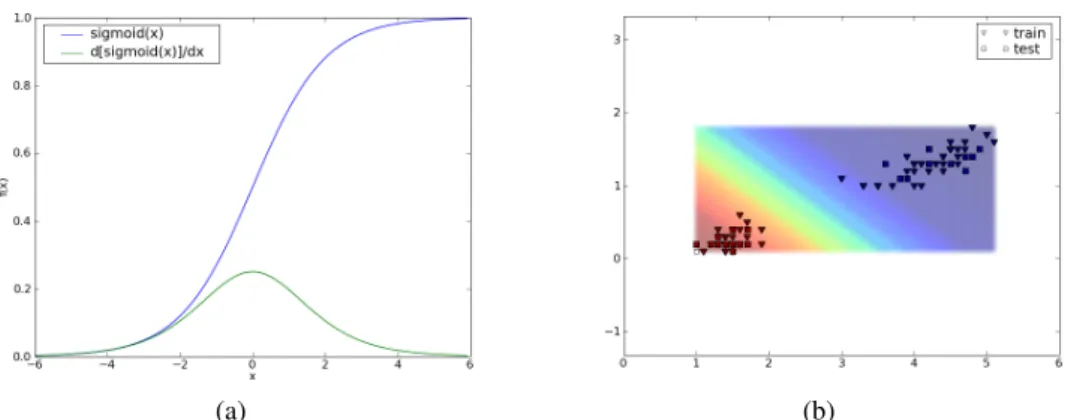
The sigmoid function is defined as sigmoid(x) = 1/(1 + e−x). As shown in
Fig-ure 1.2(a), it is a monotonically increasing function, constrained to the unit interval. Around x = 0, its behaviour is fairly linear, however its non-linearity becomes more pronounced as |x| increases. By using the conditional entropy loss function of Eq. 1.7, the loss incurred by each data point is made proportional to the log-probability mass assigned to the incorrect class.
Llog.reg.(x(i),y(i);g) = −y(i)log(g(x(i))) − (1 − y(i))log(1 − g(x(i))) (1.7)
Figure 1.2(b) shows the classification probability p(y = 1|x) for the Iris dataset. The color gradient going from bright red to dark blue corresponds to the interval of p(y = 1|x) ∈ [0,1]. We can see that the classifier has maximal uncertainty around the decision boundary.
To obtain the parameter update rules for logistic regression, we can simply perform gradient descent on R, since Llog.reg.is differentiable and smooth with respect toθ. We
obtain the following gradients onw and b: ∂R ∂wk = 1 n n
∑
i=1 [g(x(i)) − y(i)]x k (1.8) ∂R ∂b = 1 n n∑
i=1 [g(x(i)) − y(i)] (1.9)(a) (b)
Figure 1.2: (a) Sigmoid logistic function and its first derivative (b) Classification proba-bility p(y=1|x) of the logistic regression classifier, using the first two components of the Iris dataset as inputs.
1.3 Artificial Neural Networks
Artificial Neural Networks (ANN) are a natural extension of logistic regression to non-linearly separable data. For logistic regression to cope with the non-linear case, a preprocessing stage must first transform D such that the resulting dataset, D�, becomes
linearly separable. A standard linear classifier can then be used to separate D�. The
equation for thisgeneralized linear classifier is given by:
g(x) = sigmoid(
∑
j
wjφj(x) + b), (1.10)
where φ is a set of non-linear basis functions. The exact nature of φ obviously depends on the dataset, as such it would preferable to also learn this transformation from the data. We will see in the following sections that ANNs provide the mechanism for doing exactly this, by parameterizing the non-linear functionsφ as a composition of logistic classifiers.
1.3.1 Architecture
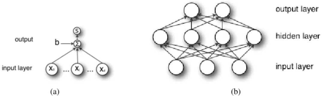
ANNs are feed-forward probabilistic models which can be used both for regression and classification. The simplest form of ANN, theMulti-Layer Perceptron is shown
in Fig. 1.3(b) (for the simplest case of one hidden layer). Comparing this figure to the graphical depiction of logistic regression (Fig. 1.3(a)), it is clear that an MLP is simply a generalized linear classifier, where the pre-processing functions φ are themselves of the formφj(x) = sigmoid(Wj·�x + bj). We will refer to the outputs of the first-layer of
logistic regressors as the hidden units, which together form the hidden layer. The output layer refers to the output of the last stage of logistic regression. In Figure 1.3(b), we have simplified the notation by merging the summation and non-linearities into a single entity, as well as omitting the contribution of the offsets bj. From looking at this
figure, it is also clear where the name "Artificial Neural Network" comes from. Much like the basic unit of the ANN, the biological neuron pools together a large number of inputs through its dendritic tree, performs a non-linear processing of its inputs (as in early integrate-and-fire models) generating an output on its single axon (through action potentials). In both cases, these units are organized into complex networks.
(a) (b)
Figure 1.3: (a) Graphical Representation of Logistic Regression. Directed connections from xj to the summation node represent the weighted contributions wjxj. s represents
the sigmoid activation function. (b) Multi-Layer Perceptron. Each unit in the hidden layer represents a logistic regression classifier. The hidden layer then forms the input to another stage of logistic classifiers.
Formally, a one-hidden layer MLP constitutes a function f : Rd → Rm, such that:
f (x) = G(b +W (s(c +V x))), (1.11)
with vectors b and c, matrices W and V and activation functions G and s (typically fixed non-linearities like the sigmoid).
While the above formulation holds true for ANNs with only a single hidden layer, extending it to the multi-layer case is fairly straightforward.
In terms of notation, the hidden units h are obtained as h(x) = s(c+V x). V ∈ Rdhxdis
the weight matrix for connections going from the input to the hidden layer. Each row Vj· of V contains the weights for the j-th hidden unit, with Vjkbeing the weight from hidden
unit hj to input xk with j ∈ [1,dh] and k ∈ [1,d]. Similarly, output units are obtained
as o(x) = G(b +W h(x)). W is the weight matrix connecting the hidden layer to output layer, with Wi jthe weights connecting output oito hidden unit hjwith i ∈ [1,m]. c ∈ Rdh
and b ∈ Rmare the offsets for the hidden and output layers respectively.
For convenience, we will define o(a)and h(a)to be the values of the output and hidden layers before their respective activation functions (i.e. o = G(o(a)),h = s(h(a))).
The exact nature of G will depend on the application. For binary classification, a single output unit suffices and G can be the sigmoid activation function. For multi-class classification, G is the softmax activation function, defined as:
softmaxi(x) = e xi
∑jexj
The single-layer MLP is of particular interest because it has been shown to be a universal approximator [27]. Given enough hidden units dh, an MLP can learn to
represent any continuous function to some fixed precision, hence capture classification boundaries of arbitrary complexity.
1.3.2 The Backpropagation Algorithm
In this section, we will briefly review the learning algorithm of ANNs. The derivation will be given for the MLP described by Eq. 1.11, with G being the identity function. This same procedure can however be generalized to any number of hidden layers and loss functions.
When the number of hidden units is fixed, MLPs are parametric models whereθ = [V,c,W,b]. As such, they can be trained to minimize the empirical risk using gradient descent. The general principle is to iteratively compute the loss L for a subset of D,
calculate the gradients∂L∂θ using thebackpropagation algorithm [54] and perform one step of gradient descent in an attempt to minimize the empirical risk R for the subsequent iteration.
Mathematically speaking, backpropagation exploits the chain-rule of derivation. We first start by writing the derivative of the loss function L (x(i),y(i); f ) with respect to the output units o(a)i . Recall that o(a)i is the activation of the units in the output layer, i.e. before the activation function (or non-linearity) has been applied.
∂L (x(i),y(i)) ∂o(a)i = ∂L ∂oi ∂oi ∂o(a)i = ∂L ∂oi �∂G(χ) ∂ χ ��� � �χ=o(a) i ≡ δi (1.12)
δirepresents the "error signal" associated with unit oi, which is back-propagated through
the network and used to tune the parameters in the lower layers. Its use is inspired from [20].
From Eq. 1.12, we can easily derive the gradients with respect to parameters [W,b] of the output layer. To simplify notation, we drop the parameters of the function L (x(i),y(i)) and simply write L .
∂L ∂bi = ∂L ∂o(a)i ∂o(a)i ∂bi =δi (1.13) ∂L ∂Wi j = ∂L ∂o(a)i ∂o(a)i ∂Wi j =δihj (1.14)
To derive the gradients on [V,c], we must first backpropagate the error ∂L∂o
i, from the
output units to the hidden units hj. From the chain-rule of derivation we can write:
∂L ∂hj =
∑
i ∂L ∂o(a)i ∂o(a)i ∂hj =∑
i δiWi j (1.15) ∂L ∂h(a)j = ∂L ∂hj ∂hj ∂h(a)j =∑
i [δiWi j]�∂s(χ)∂ χ ����� χ=h(a)j ≡ δj (1.16)Finally, from Eq. 1.16 we can now determine the gradients for the parameters [V,c] of the hidden layer:
∂L ∂cj = ∂L ∂h(a)j ∂h(a)j ∂cj =δj (1.17) ∂R ∂Vjk = ∂L ∂h(a)j ∂h(a)j ∂Vjk =δjxk (1.18) 1.3.3 Implementation Details
Combining the above equations with the gradient descent algorithm of Algorithm 1 constitutes the batch gradient descent algorithm for one-hidden layer MLPs. Algorithm 2 shows the backpropagation algorithm with stochastic updates. For each training exam-ple, we perform aforward pass to compute the predicted network output and associated loss (fprop in Algorithm 2). This loss is then used as input to the downward pass (bprop in Algorithm 2) which computes gradients for all parameters of the network. We then perform one step of stochastic gradient descent. An entire pass through the training set is referred to as anepoch. The algorithm can run for a fixed number of epochs or use a number of heuristics to decide when to stop (see section 1.3.4.2).
[37] outlines many useful tricks for making the backpropagation algorithm work bet-ter. Training patterns x should be normalized4and weights initialized to small random
values, as a function of the neuron’s fan-in. This ensures that units operate in the linear region of the sigmoid at the start of training and are thus provided with a strong learning signal. Targets y should also be chosen according to the type of non-linearity: {0,1} for the sigmoid and {−1,1} for the hyperbolic tangent tanh (an alternative to the sigmoid which is preferable according to [38]). Finally, choosing the appropriate learning rate ε is paramount to the success of this training procedure. In this thesis, we rely on first order gradient descent methods, combined with cross-validation for selecting optimal learning rates.
4Decorrelating the inputs x so that all component x
jof x are independent also helps to speedup
con-vergence [37]. However it is not clear this is advisable when working with images, since we may actually want to preserve local correlations.
Algorithm 2 TrainMLPStochastic(D,ε) Dntraining set, containing pairs (x(i),y(i))
ε learning rate
∆θminthreshold value used to detect convergence of optimization
fprop: function which computes output o(x) = f (x), according to Eq. 1.11
bprop: function which computes gradients on parameters b, W , c and V according to Eqs. 1.13-1.14 and Eqs. 1.17-1.18 respectively
Initialize c, b to zero vectors
Initialize V randomly from uniform distribution w/ range [−1/√d,+1/√d] Initialize W randomly from uniform distribution w/ range [−1/√dh, +1/√dh]
continue ← true θt−1← (W,b,V,c)
while continue do
Initialize dc,db,dV,dW to zeros for all (x(i),y(i)) in Dndo
Get next input x(i)and target y(i) from Dn
o(i)← fprop(x(i))
dW,db,dV,dc ← bprop(o(i), y(i))
(W,b,V,c) ← (W,b,V,c) − ε · (dW,db,dV,dc) end for θt ← (W,b,V,c) if |θt− θt−1| < ∆θminthen continue ← f alse end if θt−1← θt end while 1.3.4 Challenges 1.3.4.1 Local Minima
The representational power of ANNs does come at a price. Because of composing several layers of non-linearities, the optimization problem becomes non-convex. There are therefore no guarantees that the resulting solution is a global minimum. As such, when optimizing ANNs, it is customary to run several iterations of the training algorithm from different random initial weights. The performance of the network as a whole can then be reported as the mean and standard deviation of R( f ,Dtest). This allows for a fair
such as Support Vector Machines (SVM) [10]. Alternatively, one can also choose the seed used for random initialization by cross-validation.
As mentioned in section 1.1.4, stochastic gradient descent has been shown to help escape local minima. The idea is akin to Simulated Annealing [32]. By adding random-ness or noise to the gradient, we are perturbing the system in such a way as to encourage further exploration of the space. In some cases, this small perturbation will be enough to escape a shallow local minimum.
While the use of gradient descent in a non-convex setting may be objectionable to some, it is worth reminding the reader that finding the global minima is not the ultimate goal of learning. Indeed, the ultimate goal is to achieve good generalization. As such, finding a good local optimum may be sufficient.
1.3.4.2 Overfitting
ANNs being universal approximators, they are very prone to overfitting. The model selection procedure described in section 1.1.5 must therefore be used to carefully select the number of layers and number of units nhper layer. To control model capacity, ANNs
can use anearly-stopping procedure. By tracking the generalization performance during the training phase (using a validation set), it is possible to greatly reduce the sensitivity of the generalization error to the choice of network size [45]. Networks which have many more parameters than training examples can thus be used if learning is stopped before those networks are fully trained.
By tracking both training and validation errors during learning, it is possible to de-termine the optimal number of training epochse∗. During the firste∗ epochs, training
and validation errors are minimized concurrently. Aftere∗ epochs however, validation
error starts to increase (while training error is still being minimized).
Early stopping can be understood from the point of view of regularization (sec-tion 1.1.5). Since we initialize the weights to small random values, they will tend to increase throughout training. Stopping "early" (before R( fθ, D) is fully minimized) therefore prevents the parametersθ from reaching overly large values. This corresponds to an L2 regularization on the parameters [61].
1.4 Convolutional Networks
From Hubel and Wiesel’s early work on the cat’s visual cortex [29], we know there exists a complex arrangement of cells within the visual cortex. Cells are tiled in such a way as to cover the entire visual field, with each cell being only sensitive to a small sub-region called areceptive field. Two basic cell types were identified, with these very unique properties:
• simple cells (S) respond maximally to specific edge-like stimulus patterns within their receptive field. Their receptive field contains both excitatory and inhibitory regions.
• complex cells (C) respond maximally to the same set of stimulus as corresponding S cells, yet are locally invariant to their exact position.
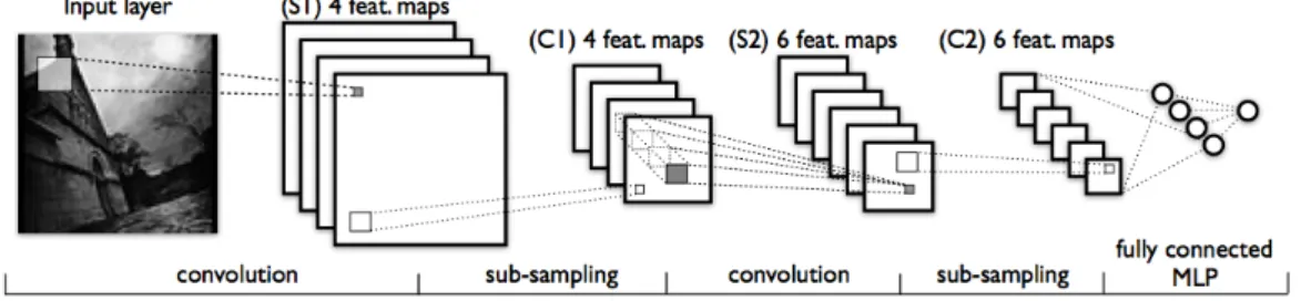
This work is at the source of many neurally inspired models of computational vi-sion: the NeoCognitron [16], HMAX [59] and LeNet-5 [40]. While they may differ in the details of their implementation, all these models share the same basic architecture, an example of which is shown in Fig. 1.4. They alternate layers of simple and complex units5, arranged in 2D grids to mimic the visual field. Each unit at layer l is connected to
a local subset of units at layer l − 1, much like the receptive fields of Hubel and Wiesel. With the exception of this local connectivity, (S) units perform the same task as the ar-tificial neurons of a standard neural network. The output of an (S) neuron can therefore be modeled with h(S)i (x) = sigmoid(∑j∈rec field of hiwi jxj+ b), where i (as well as j)
rep-resents the 2D coordinates of a neuron in the hidden and visible layers respectively. The weights of an (S) neuron therefore represent a visual feature or template to which it re-sponds maximally if present in its receptive field. (C) neurons receive the output from (S) units in their receptive fields and perform some kind of pooling function, such as computing the mean or max of their inputs. In doing so, they also act as a sub-sampling layer (i.e. fewer cells per retina area are necessary). This pooling is meant to replicate the invariance to position which was observed in (C) cells.
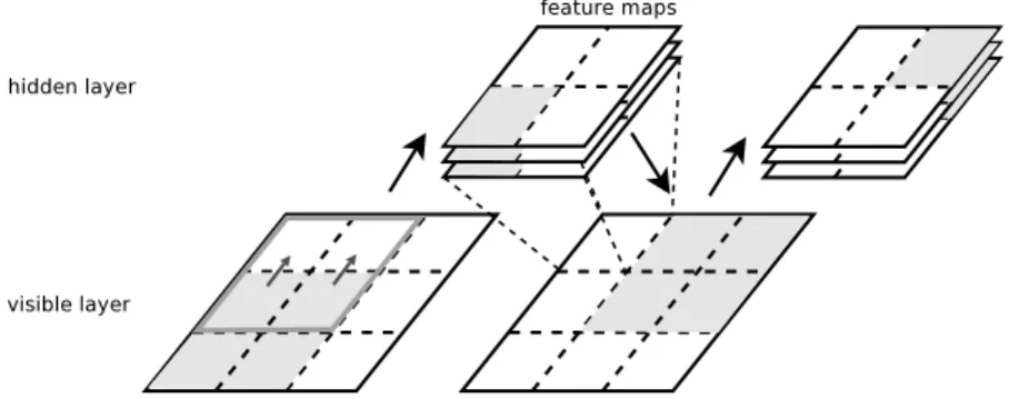
5For clarity, we use the word "unit" or "neuron" to refer to the artificial neuron and "cell" to refer to
LeNet-5 additionally adds the constraint that all (S) neurons at a given layer are "replicated" across the entire visual field. These formfeature maps which are shown in Fig. 1.4 as stacks of overlapping rectangles. (S) neurons within the same feature map share the same parameters W and each feature map contains a unique offset b. The result is aConvolutional Neural Network (CNN). CNNs get their name from the fact that the activations of neurons within feature map i can be written as hi(x) = sigmoid(Wi∗x+b),
where ∗ is the convolutional operator.
Figure 1.4: An example of a convolutional neural network, similar to LeNet-5. The CNN alternates convolutional and sub-sampling layers. Above, the input image is convolved with 4 filters generating 4 feature maps at layer (S1). Layer (C1) is then formed by down-sampling each feature map in (S1). Layer (S2) is similar to (S1), but uses 6 filters. Note that the receptive fields of units in (S2) span all 4 feature maps of (C1). The top-layers are fully-connected and form a standard MLP.
LeNet is of particular interest to this thesis, as it is the only model, of the 3 mentioned, which is trained through backpropagation. Since its inception, it has also achieved im-pressive results on a wide-array of visual recognition tasks which remain competitive to this day (0.95% classification error on MNIST [40]). The backpropagation algorithm of Eqs. 1.12-1.18. need only be modified slightly to account for the parameter sharing, by summing all parameter gradients originating from within the same feature map.
CNNs are very attractive models for vision. Features of interest (to which (S) cells are tuned) are detected regardless of the exact position of the stimulus. CNNs are thus naturally position equivariant, a property which would have had to be learnt in a tradi-tional ANN. Also, the local structure of the receptive fields exploits the local correlation present in 2D images and after training, leads tolocal feature detectors such as edges
or corners in the first layer. The pyramidal nature of CNNs also means that higher-level units learn features which are moreglobal, i.e. which span a larger field than the first layer. The pooling operation of complex cells may also provide some level of transla-tion invariance, as well as invariance to small degrees of rotatransla-tion [59]. This may help in making CNNs more robust.
Finally, CNNs massively cut-down on the amount of parameters which need to be learnt. Since we know that learning more parameters requires more training data [2], this helps the learning process. By controlling model capacity, CNNs also tend to achieve better generalization on vision problems.
1.5 Alternative Models of Computation
ANNs achieve non-linear behaviour by stacking multiple layers of simple units of the form y(x) = s(W x + b). Multiple layers are required because these simple units can only capture first-order correlations. Another solution is to usehigher-order units which capture higher-order correlations such as the covariance between all pairs of input components (xi,xj). These were first introduced in [44] under the name of HOTLU (or
high-order threshold logic unit). They showed that a simple second-order unit can learn the XOR logic function 6 in a single-pass of the training set. Formally, [17] defines
higher order units as,
yi(x) = s(T0(x) + T1(x) + T2(x) + ...) (1.19) = s(b +
∑
j Wi jxj+∑
j∑
k Wi jkxjxk+ ...) (1.20)where the maximum index of T defines the order of the unit. While Minsky and Pa-pert [44] claimed that the added complexity made them impractical to learn, Giles and Maxwell [17] showed that using prior information, higher-order units can be made in-variant to certain transformations at a relatively small price. For example, shift invari-ance can be implemented very cheaply by a second-order unit, under the conditions that
6XOR(i, j) =�+1 if sign(i)=sign( j),
{Wi jk= Wi( j−m)(k−m);m ∈ N,∀ j,k}. Having these built-in invariances is very
advanta-geous. Since the network does not have to learn them from data, higher-order units can achieve better generalization with smaller training sets.
Computational neuroscience also provides additional arguments for higher order units. While the basic artificial neural unit introduced in section 1.3 vaguely resembles the architecture and behaviour of a biological neuron, there is no doubt that the real be-haviour of a biological neuron is much more complex. Recently, Rust et al. [56] studied the behaviour of simple and complex cells in the early visual cortex of macaque mon-keys, known as V1. They showed that the behaviour of simple (S) cells accounted for several linear filters, some of which were excitatory while others were inhibitory. Their model also showed a better fit to the cell’s firing rate by taking into account pairs of filter responses. Their complete model, given in Eq. 6.1 of page 52, models cell behaviour as a weighted sum of squares of filter responses. This model will serve as inspiration to Chapter 6.
DEEP LEARNING
From the discovery of the Perceptron, to the first AI winter and the discovery of the back-propagation algorithm, the history of connectionist methods has been a very tumultuous one. The latest chapter in neural network research involves moving past the standard Multi-Layer Perceptron (MLP) and into the field ofDeep Networks: networks which are composed of many layers of non-linear transformations.
We have seen in Chapter 1 that the single-layer MLP is a universal approximator. Given enough hidden units and the ability to modify the parameters of the hidden and output layers, such MLPs can approximate any continuous function. While this revela-tion has been a strong argument in favor of neural networks, it fails to account for the complexity of the required networks. Taking inspiration from circuit theory, Håstad [19] states that a function which can be "compactly represented by a depth k architecture might require an exponential number of computational elements to be represented by a depth k − 1 architecture". To become a true universal approximator, a shallow network such as the MLP, might thus require an exponential number of hidden units. From [2], we know the amount of training data required for good generalization is proportional to the number of parameters in the network. Training shallow networks might thus require an exponential amount of training data, a seemingly prohibitive task.
To make things worse, standard training of MLPs is purely supervised. This is prob-lematic on two levels. Manual annotation of datasets is a very time-consuming and expensive task. One would thus benefit greatly from being able to use unlabeled data during the learning process. Second, it could be argued that to capture the real essence of a dataset D, one would need to model the underlying joint-probability pT(x,y). The
only learning signal used in supervised learning however, stems from the conditional-class probability p(y = m|x). Since p(x,y) = p(y|x)p(x), the use of the prior p(x) in learning thus seems attractive.
break-through in the field of deep neural networks. They introduced a greedy layer-wise train-ing procedure based on theRestricted Boltzmann Machine (RBM), which opened the door to learning deep hierarchical representations in an efficient manner. DBNs can also be used to initialize the weights of a deep feed-forward neural network. After a supervised fine-tuning stage1, this unsupervised learning procedure leads to better gen-eralization performance compared to traditional random initialization [5, 24].
The research presented in Chapters 4 and 8 was largely conducted to expand on this work. As such, this present chapter will focus on providing the reader with the necessary background material. Section 2.1 starts with an overview of Boltzmann Machines and their basic learning rule. We then proceed in section 2.2 with a short primer on Markov Chains and a particular form of Markov-Chain Monte Carlo (MCMC) sampling tech-nique known asGibbs sampling. From there, we will be able to cover the details of the DBN.
2.1 Boltzmann Machine
Boltzmann Machines (BM) [25] are probabilistic generative models which learn to model a distribution pT(x), by attempting to capture the underlying structure in the
input. BMs contain a network of binary probabilistic units, which interact through weighted undirected connections. The probability of a unit sibeing "on" given its
con-nected neighbours, is stochastically determined by the state of these neighbours, the strength of the weighted connections and the internal offset bi. Positive weights wi j
indicate a tendency for units si and sj to be "on" together, while wi j <0 indicates
some form of inhibition. The entire network defines an energy function, defined as EE(s) = −∑i∑j>iwi jsisj− ∑ibixi. The stochastic update equation is then given by:
p(si= 1|{sj: ∀ j �= i}) = sigmoid(
∑
jwi jsj+ bi), (2.1)
1The supervised fine-tuning stage consists in using the traditional supervised gradient descent
algo-rithm of section 1.3.3, using the weights learnt during the layer-wise pre-training as initial starting condi-tions.
a stochastic version of the neuronal activation function found in ANNs. Under these conditions and at a stochastic equilibrium, it can also be shown that the probability of a given global configuration is given as
p(s) = 1
Ze−EE(s). (2.2)
High probability configurations therefore correspond to low-energy states.
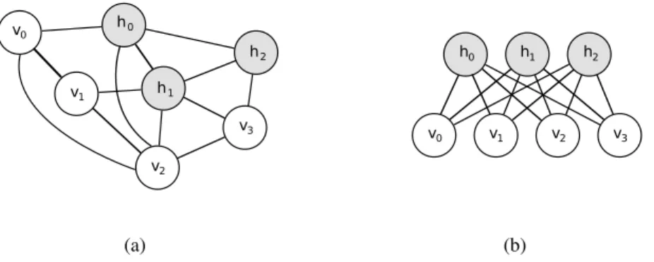
Useful learning is made possible by splitting the units intovisible and hidden units, as shown in Fig. 2.1(a), i.e. s = (v,h). During training, visible units are driven by training samples x(i)and the hidden units are left free to converge to the equilibrium distribution. The goal of learning is then to modify the network parameters θ in such a way that p(v) =∑hp(v,h) is approximately the same during training (with visible units clamped)
and when the entire network is free-running. This amounts to maximizing the empirical log-likelihood 1 N n
∑
i=1 log p(v = x(i)). (2.3)From Eq. 2.3, we can derive a stochastic gradient over the parametersθ for training example x(i): ∂log p(v) ∂θ � � � �v=x(i) = −
∑
h p(h|v = x(i))∂EE(x(i),h)
∂θ +
∑
v,hp(v,h)∂EE(v,h)
∂θ (2.4)
The above gradient is the sum of two terms, corresponding to the so-calledpositive andnegative phases. The first term is an average over p(h|v = x(i)) (i.e. probability
over the hidden units given that the visible units are clamped to training data). It will act to decrease the energy of the training examples, referred to aspositive examples. The second term, an average over p(v,h), is of opposite sign and will thus act to increase the energy of configurations sampled from the model. These configurations are referred to as negative examples, as they are training examples which the network needs to unlearn. Together, this push-pull mechanism attempts to mold an energy landscape
where configurations with visible units corresponding to training examples have low-energy and all other configurations have high-low-energy.
To apply Eq. 2.4, we must first have a mechanism for obtaining samples from p(h|v) and p(v,h). The following section covers the basic principles of Markov Chains along with the Gibbs sampling algorithm, which will prove useful for this task.
2.2 Markov Chains and Gibbs Sampling 2.2.1 Markov Chains
A Markov Chain is defined as a stochastic process {X(n): n ∈ T,X(n)∈ χ} where the distribution of the random variable X(n)depends entirely on X(n−1). This can be written
as:
p(X(n)|X(0), ...,X(n−1)) = p(X(n)|X(n−1))
The dynamics of the chain are thus entirely determined by the transition probability matrix P, whose elements pi j determine the probability of making a transition from
state i to state j. Given an initial state µ0, the distribution at step n, is thus given by
µ0Pn. Chains of interest are those which are said to be irreducible and ergodic2. Under
these conditions, a Markov chain will have a uniquestationary distribution π such that πP = π and the stationary distribution is the limiting distribution [67]. Mathematically, this translates to:
lim
n→∞P n
i j=πj, ∀i. (2.5)
An ergodic, irreducible Markov chain should therefore converge to its stationary distri-butionπ if it is run for a sufficient number of steps. This is known as the burn-in period. This leads to an important result at the foundation of most MCMC sampling methods and which will prove useful for training Boltzmann Machines.
2Simply put, irreducibility implies that all states are accessible from each other with non-null
proba-bility. Chains are said to be ergodic if they are aperiodic and have states which revisit themselves in finite time and with probability 1. For further details, we refer the reader to [67].
An important property of Markov chains, is that, for any bounded function g [67]: lim N→∞ 1 N N
∑
n=1 g(X(n)) = Eπ(g) =∑
j g( j)πj (2.6)While this only holds true in the limit of N → ∞, in practice this means that samples obtained after a sufficient burn-in period can be treated as samples fromπ. The quality of the estimate ˆEπ(g) is then determined by the mixing rate of the chain. The mixing
rate relates to the amount of correlation between consecutive samples, with good mixing corresponding to zero or low correlation. In Chapter 8, we will see that good mixing is key to the successful training of RBMs.
2.2.2 The Gibbs Sampler
For the above to be useful for training Boltzmann Machines, we still require a mech-anism for building a Markov chain with stationary distributions p(h|v) and p(v,h). This can be achieved by a process calledGibbs sampling [53]. Given a multivariate distri-bution p(X = X1, ...,Xp), the trick is to build a Markov chain with samples X(i),i ∈ N
which, given the previous value X(n) of the chain state variable, has the transition
prob-abilities as defined in Eqs. 2.7-2.10. For clarification, the superscript refers to the chain index within the Markov chain while the subscript is used to index a particular random variable (e.g. random variable formed by unit siin a Boltzmann machine)
X1(n+1)∼ p(x1|x(n)2 ,x(n)3 , ...,x(n)p ) (2.7)
X2(n+1)∼ p(x2|x(n+1)1 ,x(n)3 , ...,x(n)p ) (2.8)
... (2.9)
Xp(n+1)∼ p(xp|x1(n+1),x(n+1)2 , ...,x(n+1)p−1 ) (2.10)
Each variable is thus sampled independently, whilst keeping the other variables fixed. As an example, to sample from p(h|v) for the BM of Fig. 2.1(a), we would build a chain as stated above with X = (h0,h1,h2) and inputs v clamped. To sample from p(v,h), we
simply set X = ({vi∀i},{hj∀ j}). From Eq. 2.6, repeating the above procedure many
times results in valuesX(n)which can be treated as samples of p(h|v) and p(v,h).
Using Gibbs sampling to learn a BM is very expensive however. For each parameter update, one must run two full Markov chains to convergence, with each transition rep-resenting a full step of Gibbs sampling. For this reason, we now turn to the Restricted Boltzmann Machine, for which efficient approximations were devised.
2.3 Deep Belief Networks
This section covers the core aspects of the Deep Belief Network [26]. We start with a description of the Restricted Boltzmann Machine and show how it improves upon the generic learning algorithm of a BM. We then tackle the Contrastive Divergence algo-rithm, a trick for speeding up the learning process even further, and finally show how RBMs can be stacked to learn deep representations of data.
2.3.1 Restricted Boltzmann Machine
Restricted Boltzmann Machines are variants of BMs, where visible-visible and hidden-hidden connections are prohibited. The energy function EE(v,h) is thus defined by Eq. 2.11, whereW represents the weights connecting hidden and visible units and b, c are the offsets of the visible and hidden layers respectively.
EE(v,h) = −b�v − c�h − h�W v (2.11) The biggest advantage of such an architecture is that the hidden units become condi-tionally independent, given the visible layer (and vice-versa). This is self-evident from looking at the graphical model of Fig. 2.1(b) and may also be derived from Eqs. 2.11
(a) (b)
Figure 2.1: Example of (a) Boltzmann Machine (b) Restricted Boltzmann Machine. Visible units are shown in white and hidden units in gray. For clarity, we omit the weights on each undirected connection along with the offset.
and 2.2. We can therefore write,
p(h|v) =
∏
i p(hi|v) (2.12) p(v|h) =∏
j p(vj|h). (2.13)This greatly simplifies the learning rule of Eq. 2.4, as inference now becomes trivial and exact. As an example, we derive the gradient on Wi j. Gradients on the offsets can be
obtained in a similar manner. ∂log p(v) ∂θ � � � �v=x(i) = −
∑
h∏
i p(hi|v = x (i)) ∂EE(v,h) ∂Wi j � � � �v=x(i)+∑
v,h∏
i p(hi|v)p(v)∂EE(v,h)∂W i j (2.14) = −∑
h p(hi|x(i))hi· x(i)j +∑
v,h p(hi|v)p(v)hi· vj (2.15) = −p(hi= 1|x(i)) · x(i)j +∑
v p(hi= 1|v)p(v) · vj (2.16)= −x(i)j · sigmoid(Wi· x(i)+ ci) + Ev[p(hi|v) · vj] (2.17)
As we can see from Eq. 2.17, the positive phase gradient is straightforward to com-pute. Computing the negative phase gradient still requires samples from p(v) however.
![Figure 1.1: Linear classifier on the 2 first components of the Iris flower dataset [14].](https://thumb-eu.123doks.com/thumbv2/123doknet/12509525.341007/27.892.192.671.220.535/figure-linear-classifier-components-iris-flower-dataset.webp)