HAL Id: hal-00763488
https://hal.archives-ouvertes.fr/hal-00763488
Submitted on 13 Nov 2019
HAL is a multi-disciplinary open access
archive for the deposit and dissemination of
sci-entific research documents, whether they are
pub-lished or not. The documents may come from
teaching and research institutions in France or
abroad, or from public or private research centers.
L’archive ouverte pluridisciplinaire HAL, est
destinée au dépôt et à la diffusion de documents
scientifiques de niveau recherche, publiés ou non,
émanant des établissements d’enseignement et de
recherche français ou étrangers, des laboratoires
publics ou privés.
Comparative study with new accuracy metrics for target
volume contouring in pet image guided radiation therapy
T. Shepherd, M. Teras, R.R. Beichel, R. Boellard, M. Bruynooghe, V. Dicken,
M.J. Gooding, P.J. Julyan, J.A. Lee, Sébastien Lefèvre, et al.
To cite this version:
T. Shepherd, M. Teras, R.R. Beichel, R. Boellard, M. Bruynooghe, et al.. Comparative study with
new accuracy metrics for target volume contouring in pet image guided radiation therapy. IEEE
Transactions on Medical Imaging, Institute of Electrical and Electronics Engineers, 2012, 31 (11),
pp.2006-2024. �10.1109/TMI.2012.2202322�. �hal-00763488�
Comparative Study with New Accuracy Metrics for
Target Volume Contouring in PET Image Guided
Radiation Therapy.
Tony Shepherd, Member, IEEE, Mika Ter¨as, Member, IEEE, Reinhard R. Beichel, Member, IEEE,
Ronald Boellaard, Michel Bruynooghe, Volker Dicken, Mark J. Gooding Member, IEEE, Peter J Julyan,
John A. Lee, S´ebastien Lef`evre, Michael Mix, Valery Naranjo, Xiaodong Wu, Habib Zaidi Senior Member, IEEE,
Ziming Zeng and Heikki Minn.
Abstract—The impact of PET on radiation therapy is held 1
back by poor methods of defining functional volumes of interest. 2
Many new software tools are being proposed for contouring 3
target volumes but the different approaches are not adequately 4
compared and their accuracy is poorly evaluated due to the ill-5
definition of ground truth. This paper compares the largest cohort 6
to date of established, emerging and proposed PET contouring 7
methods, in terms of accuracy and variability. We emphasise 8
spatial accuracy and present a new metric that addresses the 9
lack of unique ground truth. 30 methods are used at 13 different 10
institutions to contour functional VOIs in clinical PET/CT and 11
a custom-built PET phantom representing typical problems in 12
image guided radiotherapy. Contouring methods are grouped 13
according to algorithmic type, level of interactivity and how they 14
exploit structural information in hybrid images. Experiments 15
reveal benefits of high levels of user interaction, as well as 16
simultaneous visualisation of CT images and PET gradients to 17
guide interactive procedures. Method-wise evaluation identifies 18
the danger of over-automation and the value of prior knowledge 19
built into an algorithm. 20
I. INTRODUCTION 21
Positron emission tomography (PET) with the metabolic
22
tracer 18
F-FDG is in routine use for cancer diagnosis and
23
treatment planning. Target volume contouring for PET
image-24
guided radiotherapy has received much attention in recent
25
years, driven by the combination of PET with CT for treatment
26
planning [1], unprecedented accuracy of intensity modulated
27
T. Shepherd, and H. Minn are with the Turku PET Centre, Turku University Hospital, and Department of Oncology and Radiotherapy, University of Turku, Finland. M. Ter¨as in with the Turku PET Centre, Turku University Hospital, Finland. R. Beichel is with the Department of Electrical & Computer Engineering and Internal Medicine, University of Iowa, USA. R. Boellaard is with the Department of Nuclear Medicine & PET Research, VU University Medical Centre, Amsterdam, The Netherlands. M. Bruynooghe is with SenoCAD Research GmbH, Germany. V. Dicken is with Fraunhofer MEVIS - Institute for Medical Image Computing, Bremen, Germany. M. J. Gooding is with Mirada Medical, Oxford, UK. P. J. Julyan is with North Western Medical Physics, Christie Hospital NHS Foundation Trust, Manchester, UK. J. A. Lee is with the Belgian FNRS and the center for Molecular Imaging, Radiotherapy, and Oncology (MIRO), Universit´e Catholique de Louvain, Brussels, Belgium. S. Lef`evre is with the VALORIA Research Laboratory, University of South Brittany, France. M. Mix is with the Department of Radi-ation Oncology, University Freiburg Medical Centre, Germany. V. Naranjo is with the Labhuman Inter-University Research Institute for Bioengineering and Human Centered Technology, Valencia, Spain. X. Wu is with the Department of Electrical & Computer Engineering, University of Iowa, USA. H. Zaidi is with the Division of Nuclear Medicine and Molecular Imaging, Geneva University Hospital, Switzerland. Z. Zeng is with the Department Computer Science, University of Aberystwyth, UK.
radiation therapy (IMRT) [2] and on-going debates [3], [4] 28
over the ability of the standardised uptake value (SUV) to 29
define functional volumes of interest (VOIs) by simple thresh- 30
olding. Many new methods are still threshold-based, but either 31
automate the choice of SUV threshold specific to an image 32
[5], [6] or apply thresholds to a combination (eg ratio) of 33
SUV and an image-specific background value [7], [8]. More 34
segmentation algorithms are entering PET oncology from 35
the field of computer vision [9] including the use of image 36
gradients [10], deformable contour models [11], [12], mutual 37
information in hybrid images [13], [14] and histogram mixture 38
models for heterogeneous regions [15], [16]. The explosion of 39
new PET contouring algorithms calls for constraint in order 40
to steer research in the right direction and avoid so-called 41
yapetism (Yet Another PET Image Segmentation Method) 42
[17]. For this purpose, we identify different approaches and 43
compare their performance. 44
Previous works to compare contouring methods in PET 45
oncology [18], [19], [20] do not reflect the wide range of 46
proposed and potential algorithms and fall short of measuring 47
spatial accuracy. [18] compare 3 threshold-based methods used 48
on PET images of non-small cell lung cancer in terms of 49
the absolute volume of the VOIs, ignoring spatial accuracy 50
of the VOI surface that is important to treatment planning. 51
Greco et al. [19] compare one manual and 3 threshold-based 52
segmentation schemes performed on PET images of head-and- 53
neck cancer. This comparison also ignores spatial accuracy, 54
being based on absolute volume of the VOI obtained by 55
manual delineation of complementary CT and MRI. Vees 56
et al. [20] compare one manual, 4 threshold-based, one 57
gradient-based and one region-growing method in segmenting 58
PET gliomas and introduce spatial accuracy, measured by 59
volumetric overlap with respect to manual segmentation of 60
complimentary MRI. However, a single manual segmentation 61
can not be considered the unique truth as manual delineation 62
is prone to variability [21], [22]. 63
Outside PET oncology, the society for Medical Image 64
Computing and Computer Assisted Intervention (MICCAI) has 65
run a ’challenge’ in recent years to compare emerging methods 66
in a range of application areas. Each challenge takes the 67
form of a double-blind experiment, whereby different methods 68
are applied by their developers on common test-data and the 69
pathological segmentation involved multiple sclerosis lesions
71
in MRI [23] and liver tumours in CT [24]. These tests
72
involved 9 and 10 segmentation algorithms respectively, and
73
evaluated their accuracy using a combination of the Dice
74
similarity coefficient [25] and Hausdorff distance [26] with
75
respect to a single manual delineation of each VOI. In 2009
76
and 2010, the challenges were to segment the prostate in
77
MRI [27] and parotid in CT [28]. These compared 2 and 10
78
segmentation methods respectively, each using a combination
79
of various overlap and distance measures to evaluate accuracy
80
with respect to a single manual ground truth per VOI. The
81
MICCAI challenges have had a major impact on segmentation
82
research in their respective application areas, but this type
83
of large-scale, double-blind study has not previously been
84
applied to PET target volume delineation for therapeutic
85
radiation oncology, and the examples above are limited by
86
their dependence upon a single manual delineation to define
87
ground truth of each VOI.
88
This paper reports on the design and results of a
large-89
scale, multi-centre, double-blind experiment to compare the
90
accuracy of 30 established and emerging methods of VOI
con-91
touring in PET oncology. The study uses a new, probabilistic
92
accuracy metric [29] that removes the assumption of unique
93
ground truth, along with standard metrics of Dice similarity
94
coefficient, Hausdorff distance and composite metrics. We use
95
both a new tumour phantom [29] and patient images of
head-96
and-neck cancer imaged by hybrid PET/CT. Experiments first
97
validate the new tumour phantom and accuracy metric, then
98
compare conceptual approaches to PET contouring by
group-99
ing methods according to how they exploit CT information in
100
hybrid images, the level of user interaction and 10 distinct
101
algorithm types. This grouping leads to conclusions about
102
general approaches to segmentation, also relevant to other tools
103
not tested here. Regarding the role of CT, conflicting reports in
104
the literature further motivate the present experiments: while
105
some authors found that PET tumour discrimination improves
106
when incorporating CT visually [30] or numerically [31],
107
others report on the detremental effect of visualising CT on
108
accuracy [32] and inter/intra-observer variability [21], [22].
109
Further experiments directly evaluate each method in terms of
110
accuracy and, where available, inter-/intra operator variability.
111
Due to the large number of contouring methods, full details
112
of their individual accuracies and all statistically significant
113
differences are provided in the supplementary material and
114
summarised in this paper.
115
The rest of this paper is organised as follows. Section
116
II describes all contouring algorithms and their groupings.
117
Section III presents the new accuracy metric and describes
118
phantom and patient images and VOIs. Experiments in section
119
IV evaluate the phantom and accuracy metric and compare
120
segmentation methods as grouped and individually. Section
121
V discusses specific findings about manual practices and the
122
types of automation and prior knowledge built into contouring
123
and section VI gives conclusions and recommendations for
124
future research in PET-based contouring methodology for
125
image-guided radiation therapy.
126
II. CONTOURINGMETHODS 127
Thirteen contouring ’teams’ took part in the experiment. We 128
identify 30 distinct ’methods’, where each is a unique com- 129
bination of team and algorithm. Table I presents the methods 130
along with labels (first column) used to identify them hereafter. 131
Some teams used more than one contouring algorithm and TABLE I: The 30 contouring methods and their attributes.
method team type interactivity CT use
max high mid low none high low none
PLa 01 PL ▲ ∎ WSa 02 WS ▲ ∎ PLb 03 PL ▲ ∎ PLc ▲ ∎ PLd ▲ ∎ T2a T2 ▲ ∎ MDa 04 MD ▲ ∎ T4a T4 ▲ ∎ T4b ▲ ∎ T4c ▲ ∎ MDb1,2 05 MD ▲ ∎ RGa RG ▲ ∎ HB 06 HB ▲ ∎ WSb 07 WS ▲ ∎ T1a 08 T1 ▲ ∎ T1b ▲ ∎ T2b T2 ▲ ∎ T2c ▲ ∎ RGb 1,2 09 RG ▲ ∎ RGc 1,2 ▲ ∎ PLe 10 PL ▲ ∎ PLf ▲ ∎ GR 11 GR ▲ ∎ MDc 12 MD ▲ ∎ T1c T1 ▲ ∎ T3a T3 ▲ ∎ T3b ▲ ∎ T2d T2 ▲ ∎ T2e ▲ ∎ PLg 13 PL ▲ ∎ 132
some well-established algorithms such as thresholding were 133
used by more than one team, with different definitions of the 134
quantity and its threshold. Methods are grouped according to 135
algorithm type and distinguished by their level of dependence 136
upon the user (section II-B) and CT data (section II-C) in 137
the case of patient images. Contouring by methods MDb, 138
RGb and RGc was repeated by two users in the respective 139
teams, denoted by subscripts 1 and 2, and the corresponding 140
segmentations are treated separately in our experiments. 141
Some of the methods are well known for PET segmentation 142
while others are recently proposed. Of the recently proposed 143
methods, some were developed specifically for PET segmen- 144
tation (e.g. GR, T2d and PLg) while some were adapted and 145
optimised for PET tumour contouring for the purpose of this 146
study. The study actively sought new methods, developed 147
or newly adapted for PET tumours, as their strengths and 148
weaknesses will inform current research that aims to refine or 149
here or not. Many of the algorithms considered operate on
151
standardised uptake values (SUVs), whereby PET voxel
in-152
tensity I is rescaled as SUV = I× (β/ain) to standardise with
153
respect to initial activity ain of the tracer in Bq ml−1 and 154
patient mass β in grams [33]. The SUV transformation only
155
affects segmentation by fixed thresholding while methods that
156
normalise with respect to a reference value in the image or
157
apply thresholds at a percentage of the maximum value are
158
invariant to the SUV transformation.
159
A. Method types and descriptions
160
Manual delineation methods (MD) use a computer mouse
161
to delineate a VOI slice-by-slice, and differ by the modes of
162
visualisation such as overlaying structural or gradient images
163
and intensity windowing. MDa is performed by a board
164
certified radiation oncologist and nuclear medicine physician,
165
who has over a decade of research and clinical experience in
166
PET-based radiotherapy planning. MDb is performed by two
167
independent, experienced physicians viewing only PET image
168
data. For each dataset, the grey-value window and level were
169
manually adjusted. MDc performed on the PET images by a
170
nuclear medicine physicist who used visual aids derived from
171
the original PET: intensity thresholds, both for the PET and
172
the PET image-gradient, were set interactively for the purpose
173
of visual guidance.
174
Thresholding methods (T1 - T4) are divided into 4 types
175
according to whether the threshold is applied to signal (T1 &
176
T2) or a combination of signal and background intensity (T3
177
& T4) and whether the threshold value is chosen a priori,
178
based on recommendations in the literature or the team’s
179
own experience (T1 & T3) or chosen for each image, either
180
automatically according to spatial criteria or visually by the
181
user’s judgement (T2 & T4). Without loss of generalisation
182
the threshold value may be absolute or percentage (e.g. of
183
peak) intensity or SUV. T1a & T1b employ the widely used
184
cut-off values of 2.5 SUV and 40% of the maximum in the
185
VOI, as used for lung tumour segmentation in [34] and [35]
186
respectively. Method T1a is the only method of all in table
187
I that is directly affected by the conversion from raw PET
188
intensity to SUVs. The maximum SUV used by method T1b
189
was taken from inside the VOI defined by T1a. To calculate
190
SUV for the phantom image, where patient weight β is
191
unavailable, all voxel values were re-scaled with respect to
192
a value of unity at one end of the phantom where intensity is
193
near uniform, causing method T1a to fail for phantom scan 2 194
as the maximum was below 2.5 for both VOIs. T1c applies
195
a threshold at 50% of the maximum SUV. Method T2a is
196
the thresholding scheme of [6], which automatically finds the
197
optimum relative threshold level (RTL) based an estimate of
198
the true absolute volume of the VOI in the image. The RTL
199
is relative to background intensity, where background voxels
200
are first labelled automatically by clustering. An initial VOI
201
is estimated by a threshold of 40% RTL, and its maximum
202
diameter is determined. The RTL is then adjusted iteratively
203
until the absolute volume of the VOI matches that of a sphere
204
of the same diameter, convolved with the point-spread function
205
(PSF) of the imaging device, estimated automatically from the
206
image. Methods T2b & T2c automatically define thresholds 207
according to different criteria. They both use the results of 208
method T1a as an initial VOI, and define local background 209
voxels by dilation. Method T2b uses two successive dilations 210
and labels the voxels in the second dilation as background. 211
The auto-threshold is then defined as 3 standard deviations 212
above the mean intensity in this background sample. Method 213
T2c uses a single dilation to define the background and finds 214
the threshold that minimises the within-class variance between 215
VOI and background using the optimization technique in [36]. 216
Finally, method T2c applies a closing operation to eliminate 217
any holes within the VOI, which may also have the effect 218
of smoothing the boundary.Method T2d finds the RTL using 219
the method of [6] in common with method T2a but with 220
different parameters and initialisation. Method T2dassumes a 221
PSF of 7 mm full width at half maximum (FWHM) rather than 222
estimating this value from the image. The RTL was initialized 223
with background defined by a manual bounding box rather 224
than clustering and foreground defined by method T3a with a 225
50% threshold rather than 40% RTL. Adaptive thresholding 226
method T2e starts with a manually defined bounding box 227
then defines the VOI by the iso-contour at a percentage of 228
the maximum value within the bounding box. Methods T3a 229
& T3b are similar to T1c, but incorporate local background 230
intensity calculated by a method equivalent to that Daisne 231
et al. [37]. A threshold value is then 41% and 50% of the 232
maximum plus background value, respectively. Method T4a 233
is an automatic SUV-thresholding method implemented in 234
the ’Rover’ software [38]. After defining a search area that 235
encloses the VOI, the user provides an initial threshold which 236
is adjusted in two steps of an iterative process. The first step 237
estimates background intensity Ib from the average intensity 238
over those voxels that are below the threshold and within 239
a minimum distance of the VOI (above the threshold). The 240
second step re-defines the VOI by a new threshold at 39% of 241
the difference Imax− Ib, where Imax is the maximum intensity 242
in the VOI. Methods T4b& T4cuse the source-to-background 243
algorithm in [8]. The user first defines a background region 244
specific to the given image, then uses parameters a and b to 245
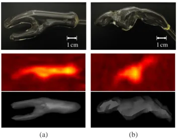
define the threshold t= aµVOI+bµBG, where µVOI+and µBGare 246
the mean SUV in the VOI and background respectively. The 247
parameters are found in a calibration procedure by scanning 248
spherical phantom VOIs of known volume. As this calibration 249
was not performed for the particular scanner used in the 250
present experiments (GE Discovery), methods T4b and T4c
251
use parameters previously obtained for Gemini and Biograph 252
PET systems respectively. 253
Region growing methods (RG) use variants of the classical 254
algorithm in [39], which begins at a ’seed’ voxel in the 255
VOI and agglomerates connected voxels until no more satisfy 256
criteria based on intensity. In RGa, the user defines a bounding 257
sphere centred on the VOI, defining both the seed at the centre 258
of the sphere and a hard constraint at the sphere surface to 259
avoid leakage into other structures. The acceptance criterion 260
is an interactively adjustable threshold and the final VOI is 261
manually modified in individual slices if needed. Methods 262
RGb & RGc use the region growing tool in Mirada XD 263
acceptance threshold defined by the user. In RGb only, the 265
results are manually post-edited using the ’adaptive brush’ tool
266
available in Mirada XD. This 3D painting tool adapts in shape
267
to the underlying image. Also in method RGbonly, CT images
268
were fused with PET for visualisation and the information used
269
to modify the regions to exclude airways and unaffected bone.
270
Watershed methods (WS) use variants of the classical
271
algorithm in [40]. The common analogy pictures a
gradient-272
filtered image as a ’relief map’ and defines a VOI as one or
273
more pools, created and merged by flooding a region with
274
water. Method WSa, adapted from the algorithm in [41] for
275
segmenting natural colour images and remote-sensing images,
276
makes use of the content as well as the location of
user-277
defined markers. A single marker for each VOI (3 × 3 or
278
5 × 5 pixels depending on VOI size) is used along with a
279
background region to train a fuzzy classification procedure
280
where each voxel is described by a texture feature vector.
281
Classification maps are combined with image gradient and the
282
familiar ’flooding’ procedure is adapted for the case of
multi-283
ple surfaces. Neither the method nor the user were specialized
284
in medical imaging. Method WSb, similar way to that in [42],
285
uses two procedures to overcome problems associated with
286
local minima in image gradient. First, viscosity is added to
287
the watershed, which closes gaps in the edge-map. Second, a
288
set of internal and external markers are identified, indicating
289
the VOI and background. After initial markers are identified
290
in one slice by the user, markers are placed automatically in
291
successive slices, terminating when the next slice is deemed
292
no longer to contain the VOI according to a large drop in
293
the ’energy’, governed by area and intensity, of the segmented
294
cross section. If necessary, the user interactively overrides the
295
automatic marker placement.
296
Pipeline methods (PL) are more complex, multi-step
algo-297
rithms that combine elements of thresholding, region growing,
298
watershed, morphological operations and techniques in [43],
299
[44], [15]. Method PLais a deformable contour model adapted
300
from white matter lesion segmentation in brain MRI. The main
301
steps use a region-scalable fitting model [45] and a global
302
standard convex scheme [46] in energy minimization based on
303
the ’Split Bregman’ technique in [43]. Methods PLb– PLdare
304
variants of the ’Smart Opening’ algorithm, adapted for PET
305
from the tool in [44] for segmenting lung nodules in CT data.
306
In contrast to CT lung lesions, the threshold used in region
307
growing can not be set a priori and is instead obtained from
308
the image interactively. Method PLb was used by an operator 309
with limited PET experience. The user of method PLc had
310
more PET experience and, to aid selection of boundary points
311
close to steep PET gradients, also viewed an overlay of local
312
maxima in the edge-map of the PET image. Finally, method
313
PLd took the results of method PLc and performed extra
pro-314
cessing by dilation, identification of local gradient maxima in
315
the dilated region, and thresholding the gradient at the median
316
of these local maxima. Methods PLe& PLf use the so-called
317
’poly-segmentation’ algorithm without and with post editing
318
respectively. PLe is based on a multi-resolution approach,
319
which segments small lesions using recursive thresholding
320
and combines 3 segmentation algorithms for larger lesions.
321
First, the watershed transform provides an initial segmentation.
322
Second, an iterative procedure improves the segmentation by 323
adaptive thresholding that uses the image statistics. Third, a 324
region growing method based on regional statistics is used. 325
The interactive variant (PLf) uses a fast interactive tool for 326
watershed-based sub-region merging. This intervention is only 327
necessary in at most two slices per VOI. Method PLg is a 328
new fuzzy segmentation technique for noisy and low resolution 329
oncological PET images. PET images are first smoothed using 330
a nonlinear anisotropic diffusion filter and added as a second 331
input to the fuzzy C-means (FCM) algorithm to incorporate 332
spatial information. Thereafter, the algorithm integrates the 333
`a trous wavelet transform in the standard FCM algorithm to 334
handle heterogeneous tracer uptake in lesions [15]. 335
The Gradient based method (GR) method is the novel 336
edge-finding method in [10], designed to overcome the low 337
signal-to-noise ratio and poor spatial resolution of PET im- 338
ages. As resolution blur distorts image features such as iso- 339
contours and gradient intensity peaks, the method combines 340
edge restoration methods with subsequent edge detection. 341
Edge restoration goes through two successive steps, namely 342
edge-preserving denoising and deblurring with a deconvo- 343
lution algorithm that takes into account the resolution of a 344
given PET device. Edge-preserving denoising is achieved by 345
bilateral filtering and a variance-stabilizing transform [47]. 346
Segmentation is finally performed by the watershed transform 347
applied after computation of the gradient magnitude. Over- 348
segmentation is addressed with a hierarchical clustering of 349
the watersheds, according to their average tracer uptake. This 350
produces a dendrogram (or tree-diagram) in which the user 351
selects the branch corresponding to the tumour or target. 352
User intervention is usually straightforward, unless the uptake 353
difference between the target and the background is very low. 354
The Hybrid method (HB) is the multi-spectral algorithm in 355
[14], adapted for PET/CT. This graph-based algorithm exploits 356
the superior contrast of PET and the superior spatial resolution 357
of CT. The algorithm is formulated as a Markov Random 358
Field (MRF) optimization problem [48]. This incorporates an 359
energy term in the objective function that penalizes the spatial 360
difference between PET and CT segmentation. 361
B. Level of interactivity 362
Levels of interactivity are defined on an ordinal scale of 363
’max’, ’high’, ’mid’,’low’ and ’none’, where ’max’ and ’none’ 364
refer to fully manual and fully automatic methods respectively. 365
Methods with a ’high’ level involve user initialisation, which 366
locates the VOI and/or representative voxels, as well as run- 367
time parameter adjustment and post-editing of the contours. 368
’Mid’-level interactions involve user-initialisation and either 369
run-time parameter adjustment or other run-time information 370
such as wrongly included/excluded voxels. ’Low’-level inter- 371
action refers to initialisation or minimal procedures to re- 372
start an algorithm with new information such as an additional 373
mouse-click in the VOI. 374
C. Level of CT use 375
We define the levels at which contouring methods exploit 376
’none’, where ’high’ refers to numerical use of CT together
378
with PET in calculations. The ’low’ group makes visual use of
379
CT images to guide manual delineation, post-editing or other
380
interactions in semi-automatic methods. The ’none’ group
381
refers to cases where CT is not used, or is viewed incidentally
382
but has no influence on contouring as the algorithm is fully
383
automatic. None of the methods operated on CT images alone.
384
III. EXPERIMENTALMETHODS
385
A. Images
386
We use two images of a new tumour phantom [29],
man-387
ufactured for this study and two clinical PET images of
388
different head-and-neck cancer patients. The test images are
389
available on-line [49], along with ground truth sets described
390
in section III-C. All imaging used the metabolic tracer 18
F-391
Fluorodeoxyglucose (FDG) and a hybrid PET/CT scanner
392
(GE Discovery), but CT images from phantom scans were
393
omitted from the test set. Table II gives more details of each
394
image type. The tumour phantom contains glass compartments
395
of irregular shapes shown in figure 1 (top row), mimicking
396
real radiotherapy target volumes. The tumour compartment
1 cm 1 cm
(a) (b)
Fig. 1: (a) tumour and (b) nodal chain VOIs of the phantom. Top: Digital photographs of glass compartments. Middle: PET images from scan 1 (sagittal view). Bottom: 3D surface view from an arbitrary threshold of simultaneous CT, lying within the glass wall.
397
(a) has branches to recreate the more complex topology of
398
some tumours. This and the nodal chain compartment (b) are
399
based on cancer of the oral cavity and lymph node metastasis
400
respectively, manually segmented from PET images of two
401
head and neck cancer patients and formed by glass blowing.
402
The phantom compartments and surrounding container were
403
filled with low concentrations of FDG and scanned by a hybrid
404
device (1, middle and bottom rows). Four phantom VOIs result
405
from scans 1 and 2, with increasing signal to background ratio
406
achieved by increasing FDG concentration in the VOIs. Details
407
of the 4 phantom VOIs are given in the first 4 rows of table
408
III. Figure 2 shows the phantom VOIs from scan 1, confirming
409
qualitatively the spatial and radiometric agreement between
410
phantom and patient VOIs.
411
TABLE III: Properties of VOI and background (BG) data (volumes in cm3 are estimated as in section III-C
VOI image initial activity (kBq ml−1) volume (cm3) source of ground truth tumour phantom 8.7 (VOI) 6.71 thresholds
node scan 1 4.9 (BG) 7.45 of
tumour phantom 10.7 (VOI) 6.71 simultaneous node scan 2 2.7 (BG) 7.45 CT image tumour patient 1 2.4 ×10⁵ 35.00 multiple node 2.54 expert tumour patient 2 3.6 ×10⁵ 2.35 delineations 0 10 20 30 0 10 20 30
distance along profile (mm)
uptake (kBq/ml)
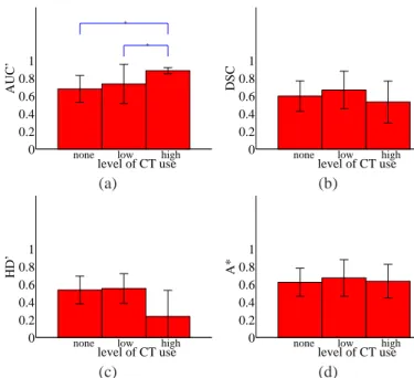
phantom patient
phantom tumour patient tumour tumour PET profiles
0 10 20 30 0
10 20 30
distance along profile (mm)
uptake (kBq/ml)
phantom patient
phantom node patient node node PET profiles
Fig. 2: Axial PET images of phantom and real tumour (top) and lymph node (bottom) VOIs with profile lines traversing each VOI. Plots on the right show the image intensity profiles sampled from each image pair.
For patient images, head and neck cancer was chosen as it 412
poses particular challenges to PET-based treatment planning 413
due to the many nearby organs at risk (placing extra demand on 414
GTV contouring accuracy), the heterogeneity of tumour tissue 415
and the common occurrence of lymph node metastasis. A large 416
tumour of the oral cavity and a small tumour of the larynx were 417
selected from two different patients, along with a metastatic 418
lymph node in the first patient (figure 3). These target volumes 419
were chosen as they were histologically proven and have a 420
range of sizes, anatomical locations/surroundings and target 421
types (tumour and metastasis). Details of the 3 patient VOIs 422
are given in the last 3 rows of table III. 423
B. Contouring 424
With the exception of the hybrid method (HB) that does not 425
apply to the PET-only phantom data, all methods contoured 426
all 7 VOIs. In the case of patient VOIs, participants had 427
the option of using CT as well as PET, and were instructed 428
to contour the gross tumour volume (GTV) and metastatic 429
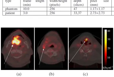
TABLE II: Details of phantom and patient PET/CT images.
Image PET (18F FDG) CT
type frame length (min) width/height (pixels) depth (slices) pixel size (mm) slice depth (mm) width/height (pixels) depth (slices) pixel size (mm) slice depth (mm) phantom 10.0 256 47 1.17×1.17 3.27 512 47 0.59×0.59 3.75 patient 3.0 256 33,37 2.73×2.73 3.27 512 42,47 0.98×0.98 1.37 (a) (b) (c)
Fig. 3: Axial neck slices of18F-FDG PET images overlain on simultaneous CT. (a) & (b) Oral cavity tumour & lymph node metastasis in patient 1 (c) Laryngeal tumour in patient 2.
methods were used at the sites of the respective teams using
431
their own software and workstations. Screen-shots of each
432
VOI were provided in axial, sagittal and coronal views, with
433
approximate centres indicated by cross-hairs and their voxel
434
coordinates provided to remove any ambiguity regarding the
435
ordering of axes and direction of increasing indices. No other
436
form of ground truth was provided. Teams were free to refine
437
their algorithms and practice segmentation before accepting
438
final contours. This practicing stage was done without any
439
knowledge of ground truth and is considered normal practice.
440
Any contouring results with sub-voxel precision were
down-441
sampled to the resolution of the PET image grid and any
442
results in mm were converted to voxel indices. Finally, all
443
contouring results were duplicated to represent VOIs first by
444
the voxels on their surface, and second by masks of the solid
445
VOI including the surface voxels. These two representations
446
were used in surface-based and volume-based contour
evalu-447
ation respectively.
448
C. Contouring evaluation
449
Accuracy measurement generally compares the contour
be-450
ing evaluated, which we denoteC, with some notion of ground
451
truth, denoted GT . We use a new probabilistic metric [29]
452
denoted AUC’, as well as a variant of the Hausdorff distance
453
[26] denoted HD’ and the standard metric of Dice similarity
454
coefficient [25] (DSC). AUC’ and HD’ are standardised to the
455
range 0 . . . 1 so that they can be easily combined or compared
456
with DSC and other accuracy metrics occupying this range
457
[50], [51], [52]. Treated separately, AUC’, HD’ and DSC
458
allow performance evaluation with and without the assumption
459
of unique ground truth, and in terms of both volumetric
460
agreement (AUC’ and DSC) and surface-displacement (HD’)
461
with respect to ground truth.
462
AUC’ is a probabilistic metric based on receiver operating
463
characteristic (ROC) analysis, in a scheme we call
inverse-464
ROC (I-ROC). The I-ROC method removes the assumption of 465
unique ground truth, instead using a set of p arbitrary ground 466
truth definitions {GTi}, i ∈ {1 . . . p} for each VOI. While 467
uniquely correct ground truth in the space of the PET image 468
would allow deterministic and arguably superior accuracy 469
evaluation, the I-ROC method is proposed for the case here, 470
and perhaps all cases except numerical phantoms, where such 471
truth is not attainable. The theoretical background of I-ROC is 472
given in Appendix A and shows that the area under the curve 473
(AUC) gives a probabilistic measure of accuracy provided that 474
the arbitrary set can be ordered by increasing volume and 475
share the topology and general form of the (unknown) true 476
surface. The power of AUC’ as an accuracy metric also relies 477
on the ability to incorporate the best available knowledge of 478
ground truth into the arbitrary set. This is done for phantom 479
and patient VOIs as follows. 480
For phantom VOIs, the ground truth set is obtained by 481
incrementing a threshold of Hounsfield units (HU) in the CT 482
data from hybrid imaging (figure 4). Masks acquired for all
(a) (b)
Fig. 4: (a) 3D visualisation of phantom VOI from CT thresh-olded at a density near the internal glass surface. (b) Arbitrary ground truth masks of the axial cross section in (a), from 50 thresholds of HU.
483
CT slices in the following steps: 484
(i) reconstruct/down-sample the CT image to the same 485
pixel grid as the PET image 486
(ii) define a bounding box in the CT image that completely 487
encloses the glass VOI as well asC 488
(iii) threshold the CT image at a value HUi 489
(iv) treat all pixels below this value as being ’liquid’ and 490
(v) label all ’liquid’ pixels that are inside the VOI as
492
positive, but ignore pixels outside the VOI.
493
(vi) repeat for p thresholds HUi, i ∈ {1 . . . p} between 494
natural limits HUmin and HUmax. 495
This ground truth set is guaranteed to pass through the internal
496
surface of the glass compartment and exploits the inherent
497
uncertainty due to partial volume effects in CT. It follows
498
from derivations in Appendix A.2-3 that AUC is equal to
499
the probability that a voxel drawn at random from below the
500
unknown CT threshold at the internal glass surface, lies inside
501
the contourC being evaluated.
502
For patient VOIs, the ground truth set is the union of
503
an increasing number of expert manual delineations. Experts
504
contoured GTV and node metastasis on PET visualised with
505
co-registered CT. In the absence of histological resection, we
506
assume that the best source of ground truth information is
507
manual PET segmentation by human experts at the imaging
508
site, who have experience of imaging the particular
tumour-509
type and access to extra information such as tumour stage,
510
treatment follow-up and biopsy where available. However, we
511
take the view that no single manual segmentation provides
512
the unique ground truth, which therefore remains unknown.
513
In total, 3 delineated each VOI on 2 occasions (denoted
514
Nexperts = 3 and Noccasions = 2) with at least a week in 515
between. The resulting set of p = Nexperts× Noccasions ground 516
truth estimates were acquired to satisfy the requirements in
517
Appendix A.3 as follows:
518
(i) define a bounding box in the CT image that completely
519
encloses all Nexperts × Noccasions manual segmentations 520
{GTi} and the contour C being evaluated 521
(ii) order the segmentations{GTi} by absolute volume in 522
cm3
523
(iii) use the smallest segmentation asGT2 524
(iv) form a new VOI from the union of the smallest and
525
the next largest VOI in the set and use this asGT3 526
(v) repeat until the largest VOI in the set has been used
527
in the union of all Nexperts× NoccasionsVOIs 528
(vi) create homogeneous masks forGT1andGTp, having 529
all negative and all positive contents respectively.
530
The patient ground truth set encodes uncertainty from inter-/intra-expert variability in manual delineation and AUC is the probability that a voxel drawn at random from the unknown manual contour at the true VOI surface, lies inside the contour C being evaluated. Finally, we rescale AUC to the range {0 . . . 1} by AUC′=AUC− 0.5 0.5 , 0≤ AUC ′ ≤ 1= maximum accuracy. (1)
Reference surfaces that profess to give the unique ground
531
truth are required to measure the Hausdorff distance and Dice
532
similarity. We obtain the ’best guess’ of the unique ground
533
truth, denoted GT∗ from the sets of ground truth definitions
534
introduced above. For each phantom VOI we select the CT
535
threshold having the closest internal volume in cm3 to an
536
independent estimate. This estimate is the mean of three
537
repeated measurements of the volume of liquid contained by
538
each glass compartment. For patient VOIs, GT∗
is the union
539
mask that has the closest absolute volume to the mean of all 540 Nexperts× Noccasionsraw expert manual delineations. 541
HD’ first uses the reference surface GT∗ to calculate the Hausdorff distance HD, being the maximum for any point on
the surface C of the minimum distances from that point to
any point on the surface ofGT∗. We then normalise HD with respect to a length scale r and subtract the result from 1 HD′=1− min(HD, r) r , 0≤ HD ′ ≤ 1= maximum accuracy, (2) where r=√3 3 4πvol(GT ∗
) is the radius of a sphere having the 542
same volume as GT∗ denoted vol(GT∗). Equation 2 trans- 543
forms HD to the desired range with 1 indicating maximum 544
accuracy. 545
DSC also uses the reference surfaceGT∗ and is calculated by
DSC= 2NC∩GT∗ NC+ NGT∗
, 0≤ DSC ≤ 1= maximum accuracy, (3)
where Nv denotes the number of voxels in volume v defined 546
by contours or their intersect. 547
Composite metrics are also used. First, we calculate a
synthetic accuracy metric from the weighted sum
A*= 0.5 AUC′+ 0.25 DSC + 0.25 HD′, (4) which, in the absence of definitive proof of their relative 548
power, assigns equal weighting to the benefits of the proba- 549
bilistic (AUC′) and deterministic approaches (DSC and HD’). 550
By complementing AUC’ with the terms using the best guess 551
of unique ground truth, A* penalises deviation from the ’true’ 552
absolute volume, which is measured with greater confidence 553
than spatial truth. Second, we create composite metrics based 554
on the relative accuracy within the set of all methods. Three 555
composite metrics are defined in table IV and justified as 556
follows: Metric n(n.s.d) favours a segmentation tool that is TABLE IV: Composite accuracy metrics that condense ranking and significance information.
n(n.s.d): the number between 0 and 4, of accuracy metrics AUC’, DSC,
HD and A*, for which a method scores an accuracy of no significant difference (n.s.d) from the best method according to that accuracy
n(>µ+σ): the number between 0 and 4, of accuracy metrics AUC’, DSC,
HD and A*, for which a method scores more than one standard deviation (σ) above the mean (µ) of that score achieved by all 32 methods (33 in the case of patient VOIs only)
median rank: the median, calculated over the 4 accuracy metrics, of
the ranking of that method in the list of all 32 methods (33 for patient VOIs only) ordered by increasing accuracy
557
as good as the most accurate in a statistical sense and, in the 558
presence of false significances due to the multiple comparison 559
effect, gives more conservative rather than falsely high scores. 560
Metric n(>µ+σ) favours the methods in the positive tails of 561
the population, which is irrespective of multiple comparison 562
effects. The rank-based metric is also immune to the multiple 563
compatrison effect and we use the median rather than mean 564
rank to avoid misleading results for a method that ranks highly 565
in only one of the metrics AUC’, DSC, HD and A*, considered 566
Intra-operator variability was measured by the raw
Haus-568
dorff distance in mm between the first and second
seg-569
mentation result from repeated contouring (no ground truth
570
necessary). However, this was only done for some contouring
571
methods. For fully automatic methods, variability is zero by
572
design and was not explicitly measured. Of the remaining
573
semi-automatic and manual methods, 11 were used twice by
574
the same operator: MDb1, MDb2, RGa, HB, WSb, RGb1, 575
RGb2, RGc1, RGc2, GR and MDc and for these we measure 576
the intra-operator variability which allows extra, direct
com-577
parisons in section IV-E.
578
IV. EXPERIMENTS
579
This section motivates the use of the new phantom and
580
accuracy metric (IV-A), then investigates contouring accuracy
581
by comparing the pooled accuracy of methods grouped
ac-582
cording to their use of CT data (section IV-B), level of user
583
interactivity (section IV-C) and algorithm type (section IV-D).
584
Section IV-E evaluates methods individually, using condensed
585
accuracy metrics in table IV. With the inclusion of repeated
586
contouring by methods MDb, RGb and RGc by a second
587
operator, there are a total of n = 33 segmentations of each
588
VOI, with the exception of phantom VOIs where n = 32 by the
589
exclusion of method HB. Also, method T1a failed to recover
590
phantom VOIs in scan 1 as no voxels were above the
pre-591
defined threshold. In this case a value of zero accuracy is
592
recorded for two out of 4 phantom VOIs.
593
A. Phantom and AUC’
594
This experiment investigares the ability of the phantom
595
to pose a realistic challenge to PET contouring, by testing
596
the null-hypothesis that both phantom and patient VOIs lead
597
to the same distribution of contouring accuracy across all
598
methods used on both image types. First, we take the mean
599
accuracy over the 4 phantom VOIs as a single score for each
600
contouring method. Next, we measure the accuracy of the same
601
methods used in patient images and take the mean over the
602
3 patient VOIs as a single score for each method. Finally,
603
a paired-samples t-test is used for the difference of means
604
between accuracy scores in each image type, with significant
605
difference defined at a confidence level of p≤ 0.05. Figure 5
606
shows the results separately for accuracy defined by AUC′, 607
DSC and HD′. There is no significant difference between
608
accuracy in phantom and patient images measured by AUC′
609
or DSC. A significant difference is seen for HD′, which
610
reflects the sensitivity of HD’ to small differences between
611
VOI surfaces. In this case the phantom VOIs are even more
612
difficult to contour accurately than the patient images, which
613
could be explained by the absence of anatomical context in
614
these images, used by operators of manual and semi-automatic
615
contouring methods. A similar experiment found no significant
616
difference between phantom and patient VOIs in terms of
617
intra-operator variability. On the whole we accept the
null-618
hypothesis meaning that the phantom and patient images pose
619
the same challenge to contouring methods in terms of accuracy
620 and variability. 621 0 0.2 0.4 0.6 0.8 1 normalised accuracy AUC’ DSC HD’ 0.684 0.646 0.607 0.618 0.54 0.496 * patient VOIs phantom VOIs
Fig. 5: Contouring accuracy in phantom and patient images, where ’⌜∗⌝’ indicates significant difference.
Figure 5 also supports the use of the new metric AUC’. 622
Although values are generally higher than DSC and HD, which 623
may be explained by the involvement of multiple ground truth 624
definitions increasing the likelihood that a contour agrees with 625
any one in the set, the variance of accuracy scores is greater for 626
AUC’ than the other metrics (table V), which indicates higher 627
sensitivity to small differences in accuracy between any two 628
methods.
TABLE V: Variance of AUC′ and standard accuracy metrics
calculated for all 7 VOIs (second column), and for the 4 and 3 VOIs in phantom and patient images respectively.
metric all VOIs phantom patient
AUC′ 0.028 0.035 0.021
DSC 0.011 0.010 0.012
HD′ 0.011 0.010 0.011
629
B. Role of CT in PET/CT contouring 630
For contouring in patient images only, we test the benefit of 631
exploiting CT information in contouring (phantom VOIs are 632
omitted from this experiments as the CT was used for ground 633
truth definitions and not made available during contouring). 634
This information is in the form of anatomical structure in the 635
case of visual CT-guidance (’low’ CT use) and higher-level, 636
image texture information in the case of method HB with 637
’high’ CT use. The null-hypothesis is that contouring accuracy 638
is not affected by the level of use of CT information. 639
We compare each pair of groups i and j that differ by CT 640
use, using a t-test for unequal sample sizes ni and nj, where 641
the corresponding samples have mean accuracy µiand µj and 642
standard deviation σi and σj. For the ith group containing 643
nmethodscontouring methods, each segmenting nVOIstargets, the 644
sample size ni = nmethods × nVOIsand µiand σj are calculated 645
over all nmethods × nVOIs accuracy scores. We calculate the 646
significance level from the t-value using the number of degrees 647
of freedom given by the Welch-Satterthwaite formula for un- 648
differences between groups are defined by confidence interval
650
of p ≤ 0.05. For patient images only, nVOIs = 3 and for the
651
grouping according to CT use in table I, nmethods= 1, 6 and 26 652
for the groups with levels of CT use ’high’, ’low’ and ’none’
653
respectively (methods RGbin the ’low’ group and MDb& RGc
654
in the ’none’ group were used twice by different operators in
655
the same team). We repeat for 4 accuracy metrics AUC′, DSC,
656
HD′ and their weighted sum A*. Figure 6 shows the results
657
for all groups ordered by level of CT use, in terms of each
658
accuracy metric in turn.
0 0.2 0.4 0.6 0.8 1 AUC’ level of CT use none low high
* * 0 0.2 0.4 0.6 0.8 1 DSC level of CT use none low high
(a) (b) 0 0.2 0.4 0.6 0.8 1 HD’ level of CT use
none low high 0
0.2 0.4 0.6 0.8 1 A* level of CT use none low high
(c) (d)
Fig. 6: Effect of CT use on contouring accuracy in patient images, measured by (a) AUC′, (b) DSC, (c) HD′and (d) A*, where ’⌜∗⌝’ denotes ignificant difference between two levels of CT use.
659
With the exception of AUC’ the use of CT as a visual
660
guidance (’low’), out-performed the ’high’ and ’none’ groups
661
consistently but without significant difference. The fact that the
662
’high’ group (method HB only) significantly out-performed
663
the lower groups in terms of AUC’ alone indicates that the
664
method had good spatial agreement with one of the
union-of-665
experts masks for any given VOI, but this union mask did not
666
have absolute volume most closely matching the independent
667
estimates used in calculations of DSC and HD’. We conclude
668
that the use of CT images as visual reference (’low’ use)
669
generally improves accuracy, as supported by the consistent
670
improvement in 3 out of 4 metrics. This is in agreement
671
with experiments in [30] and [31], which found the benefits
672
of adding CT visually and computationally, in manual and
673
automatic tumour delineation and classification respectively.
674
C. Role of user interaction
675
This experiment investigates the affect of user-interactivity
676
on contouring performance. The null hypothesis is that
con-677
touring accuracy is not affected by the level of interactivity
678
in a contouring method. We compare each pair of groups i
679
and j that differ by level of interactivity, using a t-test for 680
unequal sample sizes as above. For the grouping according 681
to level of interactivity in table I, groups with interactivity 682
level ’max’, ’high’, ’mid’, ’low’ and ’none’ have nmethods = 683
4, 3, 7, 13 (12 for phantom images by removal of method 684
HB) and 6 respectively (methods MDb, RGMDband RGMDc 685
in the ’max’, ’high’ and ’mid’ groups respectively were used 686
twice by different operators in the same team). We repeat for 687
patient images (nVOIs = 3), phantom images (nVOIs = 4) and 688
the combined set (nVOIs = 7) and, as above, for each of the 689
4 accuracy metrics. Figure 7 shows all results for all groups 690
ordered by level of interactivity. 691
The trends for each of phantom, patient and all VOIs 692
are consistent over all metrics. The most accurate methods 693
were those in the ’high’ and ’max’ groups for phantom and 694
patient images respectively. For patient images, the ’max’ 695
group is significantly more accurate than any other and this 696
trend carries over to the pooled accuracies in both image 697
types despite having less patient VOIs (n = 3) than phantom 698
VOIs (n = 4). For phantom VOIs, with the exception of HD’, 699
there are no significant differences between ’high’ and ’max’ 700
groups and these both significantly out-perform the ’low’ and 701
’none’ groups in all metrics. For HD’ alone, fully manual 702
delineation is significantly less accurate than semi-automatic 703
methods with ’high’ levels of interaction. This may reflect the 704
lack of anatomical reference in the phantom images, which 705
is present for patient VOIs and guides manual delineation. 706
As high levels of interaction still appear most accurate, the 707
reduced accuracy of fully manual methods is not considered 708
likely to be caused by a bias of manual delineations toward 709
manual ground truth, given the levels of inter-user variability. 710
Overall, we conclude that manual delineation is more accurate 711
than semi- or fully-automatic methods, and that the accuracy of 712
semi-automatic methods improves with the level of interaction 713
built in. 714
D. Accuracy of algorithm types 715
This experiment compares the accuracy of different al- 716
gorithm types, defined in section II-A. The null hypothesis 717
is that contouring accuracy is the same for manual or any 718
numerical method regardless of the general approach they 719
take. We compare each pair of groups i and j that differ 720
by algorithm type, using a t-test for unequal sample sizes as 721
above. For the grouping according to algorithm type in table I, 722
nmethods = 4,3,5,2,3,5,2,1,1 (0 for phantom images by removal 723
of method HB) and 7 for algorithm-types MD, T1, T2, T3, 724
T4, RG, WS, GR, HB and PL respectively (methods MDb in 725
the MD, and RGb& RGcin the RG group were used twice by 726
different operators in the same team). As above, we repeat for 727
patient images (nVOIs = 3), phantom images (nVOIs = 4) and 728
the combined set (nVOIs = 7), and for each of the 4 accuracy 729
metrics. Figure 8 shows the results separately for all image 730
sets and accuracy metrics. 731
Plot (b) reproduces the same anomalous success of the 732
hybrid method (HB) in terms of AUC’ alone, as explained 733
above. Manual delineation exhibits higher accuracy than other 734
0 0.2 0.4 0.6 0.8 1 Phantom VOIs AUC’
level of user interaction none low medium high max
* * * * * * 0 0.2 0.4 0.6 0.8 1 Patient VOIs AUC’
level of user interaction none low medium high max
* * * * 0 0.2 0.4 0.6 0.8 1 All VOIs AUC’
level of user interaction none low medium high max
* * * (a) (b) (c) 0 0.2 0.4 0.6 0.8 1 DSC
level of user interaction none low medium high max
* * * * * * 0 0.2 0.4 0.6 0.8 1 DSC
level of user interaction none low medium high max
* * * * 0 0.2 0.4 0.6 0.8 1 DSC
level of user interaction none low medium high max
* * * * * (d) (e) (f) 0 0.2 0.4 0.6 0.8 1 HD’
level of user interaction none low medium high max
* * * * * * * 0 0.2 0.4 0.6 0.8 1 HD’
level of user interaction none low medium high max
* * * * * * 0 0.2 0.4 0.6 0.8 1 HD’
level of user interaction none low medium high max
* * * * * * (g) (h) (i) 0 0.2 0.4 0.6 0.8 1 A*
level of user interaction none low medium high max
* * * * * * * 0 0.2 0.4 0.6 0.8 1 A*
level of user interaction none low medium high max
* * * * 0 0.2 0.4 0.6 0.8 1 A*
level of user interaction none low medium high max
* *
* *
(j) (k) (l)
Fig. 7: Effect of user interaction on contouring accuracy measured by top row: AUC′for (a) phantom, (b) patient and (c) both VOI types, second row: DSC for (d) phantom (e) patient and (f) both image types, third row: HD′for (g) phantom, (h) patient and (i) both image types, and bottom row: A* for (j) phantom, (k) patient and (l) both VOI types. Significant differences between any two levels of user interaction are indicated by ’⌜∗⌝’.
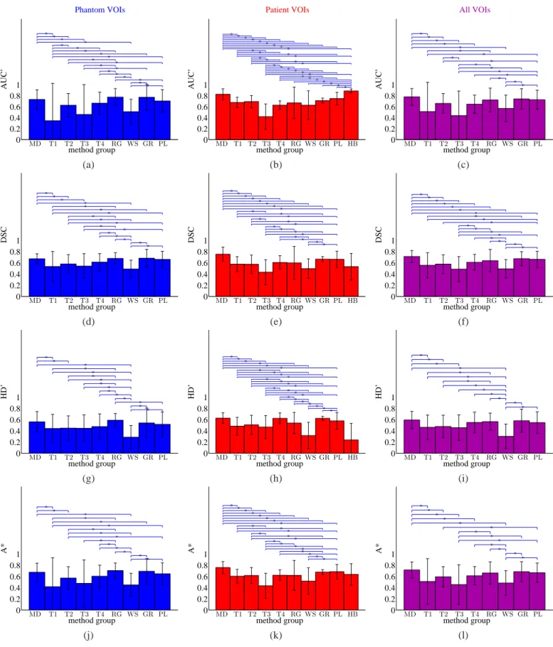
0 0.2 0.4 0.6 0.8 1 Phantom VOIs AUC’ method group MD T1 T2 T3 T4 RG WS GR PL * * * * * * * * * * * * * * * * * * * 0 0.2 0.4 0.6 0.8 1 Patient VOIs AUC’ method group MD T1 T2 T3 T4 RG WS GR PL HB * * * * * * * * * * * * * * * * * * * * * * * * * * * * * * 0 0.2 0.4 0.6 0.8 1 All VOIs AUC’ method group MD T1 T2 T3 T4 RG WS GR PL * * * * * * * * * * * * * * * * (a) (b) (c) 0 0.2 0.4 0.6 0.8 1 DSC method group MD T1 T2 T3 T4 RG WS GR PL * * * * * * * * * * * * * * * * * 0 0.2 0.4 0.6 0.8 1 DSC method group MD T1 T2 T3 T4 RG WS GR PL HB * * * * * * * * * * * * * * * * * * * * * * 0 0.2 0.4 0.6 0.8 1 DSC method group MD T1 T2 T3 T4 RG WS GR PL * * * * * * * * * * * * * * * * * * (d) (e) (f) 0 0.2 0.4 0.6 0.8 1 HD’ method group MD T1 T2 T3 T4 RG WS GR PL * * * * * * * * * * * * * * * 0 0.2 0.4 0.6 0.8 1 HD’ method group MD T1 T2 T3 T4 RG WS GR PL HB * * * * * * * * * * * * * * * * * * * * * * * * * 0 0.2 0.4 0.6 0.8 1 HD’ method group MD T1 T2 T3 T4 RG WS GR PL * * * * * * * * * * * * * (g) (h) (i) 0 0.2 0.4 0.6 0.8 1 A* method group MD T1 T2 T3 T4 RG WS GR PL * * * * * * * * * * * * * * * 0 0.2 0.4 0.6 0.8 1 A* method group MD T1 T2 T3 T4 RG WS GR PL HB * * * * * * * * * * * * * * * * * * * * * * 0 0.2 0.4 0.6 0.8 1 A* method group MD T1 T2 T3 T4 RG WS GR PL * * * * * * * * * * * * * (j) (k) (l)
Fig. 8: Contouring accuracy of all algorithm types measured by top row: AUC′ for (a) phantom, (b) patient and (c) both VOI types, second row: DSC for (d) phantom (e) patient and (f) both image types, third row: HD′for (g) phantom, (h) patient and (i) both image types and bottom row: A* for (j) phantom, (k) patient and (l) both VOI types. Significant differences between any two algorithm types are indicated by ’⌜∗⌝’.
in phantom images and the top two for any metric in patient
736
images. The pooled results over all images reveal manual
737
delineation as the most accurate in terms of all 4 metrics. With
738
the exception of T4 in terms of HD’ (patient and combined
739
image sets), the improvement of manual delineation over any
740
of the thresholding variants T1 - T4 is significant, despite
741
these being the most widely used (semi-)automatic methods. A
742
promising semi-automatic approach is the gradient-based (GR)
743
group (one method), which has the second highest accuracy
744
by all metrics for the combined image set and significant
745
difference from manual delineation. Conversely, the watershed
746
group of methods that also rely on image gradients exhibit
747
consistently low accuracy. This emphasized the problem of
748
poorly-defined edges and noise-induced false edges typical
749
of PET gradient filtering, which in turn suggests that
edge-750
preserving noise reduction by the bi-lateral filter plays a large
751
part in the success of method GR.
752
E. Accuracy of individual methods
753
The final experiments directly compare the accuracy of
754
all methods. Where two algorithms have arguably minor
755
difference, as in the case of PLc and PLd which differ by
756
an extra processing step applied by PLd, these are treated as
757
separate methods because the change in contouring results is
758
notable and can be attributed to the addition of the processing
759
step, which is informative. Repeated segmentations by two
760
different users in the cases of methods MDb
1,2, RGb1,2 and 761
RGc
1,2are counted as two individual results so there are a total 762
of n = 32 ’methods’, or n = 33 for patient VOIs in PET/CT
763
only by inclusion of hybrid method HB. The null hypothesis
764
is that all n cases are equally accurate. We compare each pair
765
of methods i and j that differ by method, using a t-test for
766
equal sample sizes ni = nj = nVOIs, where mean accuracy 767
µi and µj and standard deviation σi and σj are calculated 768
over all VOIs and there are 2nVOIs− 2 degrees of freedom. 769
As above, we repeat for all image sets and accuracy metrics.
770
Figure 9 shows the results separately for phantom, patient and
771
combined image sets in terms of A* only. Full results for all
772
metrics and significant differences between methods are given
773
in the supplementary material.
774
The generally low values of A* in figure 9 and other
775
metrics in the supplementary material highlight the problem
776
facing accurate PET contouring. These results also reiterate
777
the general finding that manual practices can be more accurate
778
than semi- or fully-automatic contouring. For patient images,
779
and the combined set, the most accurate contours are manually
780
delineated by method MDc. Also for these image sets the
781
second and third most accurate are another manual method
782
(MDb2) and the ’smart opening’ algorithm (PLb) with mid-783
level interactivity.
784
For phantom VOIs only, methods RGb and T1b, with
high-785
and low-level interactivity, out-perform manual method MDc
786
with no significant difference. Method RGb is based on SRG
787
with post-editing by the adaptive brush and showed low
788
accuracy for patient VOIs with RGb2 being significantly less 789
accurate than the manual method MDc (see supplementary
790
material). Method T1b is based on thresholding and showed
791
low accuracy for patient VOIs, being significantly less accurate 792
than the manual methods MDc and MDb2 (see supplementary 793
material). Their high accuracy in phantom images alone could 794
be explained by methods T1b and RGb being particularly 795
suited to the relative homogeneity of the phantom VOIs. 796
Methods WSa, T1c and T3b have the 3 lowest accuracies 797
by mean A* across all 3 image sets. The poor performance 798
of method WSa could be explained by its origins (colour 799
photography and remote-sensing) and user having no roots 800
or specialism in medical imaging. Threshold methods T1c 801
and T3b give iso-contours at 50% of the local peak intensity 802
without and with adjustment for background intensity respec- 803
tively. Their poor performance in all image types highlights 804
the limitations of thresholding. 805
Table VI presents the composite metrics explained in section 806
III-C along with intra-operator variability where available (last 807
two columns), measured by the Hausdorff distance in mm 808
between two segmentations of the same VOI, averaged over 809
the 3 patient or 4 phantom VOIs. This definition of intra- 810
operator variability gives an anomalously high value if the two 811
segmentations resulting from repeated contouring of the same 812
VOI do not have the same topology, as caused by an internal 813
hole in the first contouring by method RGb1. Notably, we find 814
no correlation between intra-operator variability and the level 815
of interactivity of the corresponding methods. The same is 816
true for inter-operator variability (not shown) calculated by 817
the Hausdorff distance between segmentations by different 818
users of the same method (applicable to methods MDb, RGb 819
and RGc). This finding contradicts the general belief that 820
user input should be minimised to reduce variability. Table 821
VI reaffirms the finding that manual delineation is the most 822
accurate method type, with examples MDcand MDb1,2scoring 823
highly in all metrics. The most consistently accurate non- 824
manual methods are the semi- and fully-automatic methods 825
PLb and PLc. More detailed method-wise comparisons are 826
made in the next section. 827
V. DISCUSSION 828
We have evaluated and compared 30 implementations of 829
PET segmentation methods ranging from fully manual to fully 830
automatic and representing the range from well established 831
to never-before tested on PET data. Region growing and 832
watershed algorithms are well established in other areas of 833
medical image processing, while their use for PET target 834
volume delineation is relatively new. Even more novel ap- 835
proaches are found in the ’pipeline’ group and the two distinct 836
algorithms of gradient-based and hybrid segmentation. The 837
gradient-based method [10] has already had an impact in the 838
radiation oncology community and the HB method [14] is one 839
of few in the literature to make numerical use of the structural 840
information in fused PET/CT. The multispectral approach is in 841
common with classification experiments in [13] that showed 842
favourable results over PET alone. 843
A. Manual delineation 844
Free-hand segmentation produced among the most accu- 845