Feedforward deep architectures for classification and synthesis

(1)

Universit´e de Montr´eal

par David Warde-Farley

Département d’informatique et de recherche opérationnelle Faculté des arts et des sciences

Thèse présentée à la Faculté des arts et des sciences en vue de l’obtention du grade de Philosophiæ Doctor (Ph.D.)

en informatique

aoˆut, 2017

(2)

Résumé

Cette thèse par article présente plusieurs contributions au domaine de l’ap-prentissage de représentations profondes, avec des applications aux problèmes de classification et de synthèse d’images naturelles. Plus spécifiquement, cette thèse présente plusieurs nouvelles techniques pour la construction et l’entraˆınement de réseaux neuronaux profonds, ainsi qu’une étude empirique de la technique de «dro-pout», une des approches de régularisation les plus populaires des dernières années. Le premier article présente une nouvelle fonction d’activation linéaire par mor-ceau, appellée«maxout», qui permet à chaque unité cachée d’un réseau de neurones d’apprendre sa propre fonction d’activation convexe. Nous démontrons une perfor-mance améliorée sur plusieurs tâches d’évaluation du domaine de reconnaissance d’objets, et nous examinons empiriquement les sources de cette amélioration, y compris une meilleure synergie avec la méthode de régularisation «dropout» ré-cemment proposée.

Le second article poursuit l’examen de la technique «dropout». Nous nous concentrons sur les réseaux avec fonctions d’activation rectifiées linéaires (ReLU) et répondons empiriquement à plusieurs questions concernant l’efficacité remar-quable de «dropout» en tant que régularisateur, incluant les questions portant sur la méthode rapide de rééchelonnement au temps de l’évaluation et la moyenne géométrique que cette méthode approxime, l’interprétation d’ensemble comparée aux ensembles traditionnels, et l’importance d’employer des critères similaires au «bagging» pour l’optimisation.

Le troisième article s’intéresse à un problème pratique de l’application à l’échelle industrielle de réseaux neuronaux profonds au problème de reconnaissance d’objets avec plusieurs étiquettes, nommément l’amélioration de la capacité d’un modèle à discriminer entre des étiquettes fréquemment confondues. Nous résolvons le pro-blème en employant la prédiction du réseau pour construire une partition de l’es-pace des étiquettes et ajoutons au réseau des sous-composantes dédiées à chaque sous-ensemble de la partition.

Finalement, le quatrième article s’attaque au problème de l’entraˆınement de modèles génératifs implicites sur des images naturelles en suivant le paradigme des réseaux génératifs adversariaux (GAN) récemment proposé. Nous présentons une procédure d’entraˆınement améliorée employant un auto-encodeur débruitant, entraˆıné dans un espace de caractéristiques abstrait appris par le discriminateur, pour guider le générateur à apprendre un encodage qui s’aligne de plus près aux données. Nous évaluons le modèle avec le score «Inception» récemment proposé.

(3)

Mots-clés: apprentissage de représentations profondes, apprentisage machine, réseau de neurones, apprentisage supervisé, apprentissage non-supervisé, dropout, fonction d’activation, réseau convolutionel, reconnaissance d’objets, synthèse d’images

(4)

Summary

This thesis by articles makes several contributions to the field of deep learning, with applications to both classification and synthesis of natural images. Specifically, we introduce several new techniques for the construction and training of deep feed-forward networks, and present an empirical investigation into dropout, one of the most popular regularization strategies of the last several years.

In the first article, we present a novel piece-wise linear parameterization of neural networks, maxout, which allows each hidden unit of a neural network to e↵ectively learn its own convex activation function. We demonstrate improvements on several object recognition benchmarks, and empirically investigate the source of these improvements, including an improved synergy with the recently proposed dropout regularization method.

In the second article, we further interrogate the dropout algorithm in particular. Focusing on networks of the popular rectified linear units (ReLU), we empirically examine several questions regarding dropout’s remarkable e↵ectiveness as a regu-larizer, including questions surrounding the fast test-time rescaling trick and the geometric mean it approximates, interpretations as an ensemble as compared with traditional ensembles, and the importance of using a bagging-like criterion for op-timization.

In the third article, we address a practical problem in industrial-scale application of deep networks for multi-label object recognition, namely improving an existing model’s ability to discriminate between frequently confused classes. We accomplish this by using the network’s own predictions to inform a partitioning of the label space, and augment the network with dedicated discriminative capacity addressing each of the partitions.

Finally, in the fourth article, we tackle the problem of fitting implicit generative models of open domain collections of natural images using the recently introduced Generative Adversarial Networks (GAN) paradigm. We introduce an augmented training procedure which employs a denoising autoencoder, trained in a high-level feature space learned by the discriminator, to guide the generator towards feature encodings which more closely resemble the data. We quantitatively evaluate our findings using the recently proposed Inception score.

Keywords: neural network, machine learning, deep learning, supervised learning, unsupervised learning, dropout, generative adversarial network, activation func-tion, convolutional network, object recognifunc-tion, image synthesis

(5)

List of Figures

1.1 An example of a directed graphical model . . . 7

1.2 General form of a directed latent variable model . . . 9

1.3 The Bayes-ball algorithm for conditional independence testing. . . . 10

1.4 Polar coordinates vs. Cartesian coordinates . . . 11

1.5 Penalized autoencoders and denoising autoencoders . . . 16

3.1 Using maxout to implement pre-existing activation functions . . . . 24

3.2 The activations of maxout units are not sparse. . . 24

3.3 Universal approximator network . . . 25

3.4 Example maxout filters . . . 26

3.5 CIFAR-10 learning curves . . . 30

3.6 Comparison to rectifier networks. . . 37

3.7 Monte Carlo classification . . . 38

3.8 KL divergence from Monte Carlo predictions . . . 39

3.9 Optimization of deep models . . . 40

3.10 Avoidance of “dead units” . . . 41

5.1 Exhaustive enumeration of masks vs. weight-scaling . . . 51

5.2 Comparison of arithmetic vs. geometric means over masks . . . 52

5.3 Comparing dropout to untied-weight dropout ensembles. . . 54

5.4 Dropout and dropout boosting vs. SGD . . . 57

7.1 Illustration of the network augmentation process . . . 63

7.2 Evaluation of the trained model on ImageNet classification . . . 66

10.1 CIFAR-10 samples . . . 90

10.2 STL-10 samples . . . 92

(9)

List of Tables

3.1 Permutation invariant MNIST classification . . . 27

3.2 Convolutional MNIST classification . . . 28

3.3 CIFAR-10 classification . . . 29

3.4 CIFAR-100 classification . . . 31

3.5 SVHN classification . . . 31

7.1 Examples of discovered label-space clusters . . . 65

7.2 Augmented network mAP and computational footprint . . . 66

10.1 Inception scores for generative models of CIFAR-10 . . . 91

10.2 Inception scores for generative models of STL-10 . . . 91

(10)

List of Abbreviations

ALI Adversarially Learned Inference CNN Convolutional Neural Network DBM Deep Boltzmann Machine

GAN Generative Adversarial Network GPU Graphics Processing Unit

i.i.d. Independent and Identically Distributed

ILSVRC ImageNet Large-Scale Visual Recognition Challenge KL Kullback-Leibler (divergence)

LAPGAN Laplacian Pyramid Generative Adversarial Network mAP Mean Average Precision

MLP Multi-Layer Perceptron

MP-DBM Multi-Prediction Deep Boltzmann Machine NCE Noise-Contrastive Estimation

PWL Piecewise Linear RGB Red, Green, Blue ReLU Rectified Linear Unit

SGD Stochastic Gradient Descent SVHN Street View House Numbers

SVM Support Vector Machine VAE Variational Auto-Encoder

(11)

Acknowledgments

Much of the credit for my reaching this point is due to my mother, Joan Warde-Farley, and my father, the late Bernard Leo Farley.

My mother has been a constant source of support throughout this degree and the two preceding it, and guided us adeptly through the passing of my father in 2005. Among other traits, I have inherited her unmatched stubbornness: having surreptitiously overheard her expressing doubt in my seriousness about pursuing a PhD in Montreal, I knew for certain that I had to carry it forward. Her early incredulity of course gave way to a deluge of financial, logistical, emotional and moral support, as I always knew it would.

My father taught me a great deal during the two decades we shared, including the value of honesty, humility, perseverance, and clarity of purpose. I remain but an imperfect student of his ways. I trust that he would view the first doctorate on his side of the family as a compelling alternative to the career as a concert pianist that he once envisioned for me.

I would like to earnestly thank my doctoral advisor, Yoshua Bengio, for his encouragement, enthusiasm, patience, and guidance, for granting me the great pleasure of joining MILA (n´ee LISA), and for being the organizing force thereof. It has been an immense honour to witness firsthand the lab’s transformation into the deep learning juggernaut that it is today. I’d also like to extend a special thanks to Aaron Courville, with whom I interacted a great deal in the early days of my studies, and with whom I co-authored several of the articles presented herein, and to Vincent Dumoulin for his assistance in translating the summary of this thesis.

I have had the enormous fortune to benefit from many brilliant teachers and mentors even before my arrival in Montreal. In particular, I’d like to particularly thank Quaid Morris, my MSc supervisor, from whom I learned a great deal about being a scientist, and who encouraged me to pursue my interests even where they diverged from his own; the late Sam Roweis, whose contagious enthusiasm was matched only by the incredible depth and breadth of his scholarship, may he rest in peace; and Geo↵rey Hinton, scientific renegade extraordinaire, who originally ignited my interest in machine learning and neural networks.

Part of this work was undertaken at Google in Mountain View, California. I’d like to thank everyone with whom I interacted during both of my internships, on the Brain team and the Image Understanding team respectively, and in particular my hosts, Rajat Monga and Drago Anguelov, as well as Andrew Rabinovich with whom I worked closely during the summer of 2014.

I am grateful to all the members of MILA, past and present, with whom I have interacted. Many of the lab’s members became good friends outside of the context of the lab. I would in particular like to thank Ian Goodfellow, Guillaume Desjardins, Razvan Pascanu, Mehdi Mirza, Laurent Dinh, Vincent Dumoulin, Mathieu Ger-main, Li Yao, Yann Dauphin, Bart van Merri¨enboer and Yaroslav Ganin for their

(12)

extralaboratory camaraderie. I am delighted to be reunited with numerous MILA colleagues in my new position at DeepMind.

Certain individuals have gone beyond mere friendship and played pivotal roles in my years in Montreal, and may be unaware just how deeply certain small acts have shaped my life for the better. In that vein, I owe a particular debt of gratitude to each of James Bergstra and Dumitru Erhan.

All of the work in these pages is built upon open source scientific software, a noble cause to which I have done my best to contribute (sometimes at the expense of more pressing pursuits, in the finest of graduate school traditions). I would like to thank in particular all of the contributors to NumPy, SciPy, Matplotlib and IPython. I would especially like to thank the Theano core development team (notably Frédéric Bastien, Pascal Lamblin, Arnaud Bergeron) for all of their hard work on a tool that played an integral role in much of this research, as well as Ian Goodfellow, Vincent Dumoulin, Matt Grimes and others for their contributions to Pylearn2 alongside my own. It has also been a great pleasure to collaborate with Bart van Merriënboer, Dzmitry Bahdanau, Vincent Dumoulin, and Dmitriy Serdyuk on the Blocks and Fuel packages, which restored sanity to my research workflow.

I would like to graciously acknowledge financial support from Ubisoft, D-Wave Systems, the Canada Research Chairs, NSERC, CIFAR, and the Universit´e de Montr´eal. I’d also like to thank Enthought Inc. for sponsoring my attendance of SciPy 2008 through 2012.

Last but not least, I’d like to thank my fianc´ee, Johanna, for her love and support, and Sheldon for his life-enriching a↵ection and mischief.

(13)

1

Background

Machine learning is the study of artificial systems that can adapt or learn from data presented to them. In the seminal work of Valiant (1984), the definition of learning adopted is somewhat open-ended, but appropriate given the topics covered herein: “a program for performing a task has been acquired by learning if it has been acquired by any means other than explicit programming”. Machine learning, in its various guises, has established itself as a near-ubiquitous tool in science and engineering, easing the development and deployment of automated systems for tasks where explicitly articulated “recipes” are difficult (or e↵ectively impossible, a priori) to construct. Insofar as any agent considered intelligent ought to be able (and should frequently find it useful) to adapt its behaviour in light of observation and experience, the study of machine learning is an essential element in the pursuit of artificial intelligence.

The academic study of machine learning is commonly broken down into three main areas. Supervised learning deals with the discovery of input-output mappings for some task of interest given correct or approximately correct examples of said mapping. The setting in which a system predicts one of a fixed number of discrete labels given an input signal (such as predicting, from physiological measurements, the presence or absence of a disease) is commonly referred to as classification, whereas prediction involving well-ordered numerical targets (a company’s stock price, for example) is known as regression. Unsupervised learning is an umbrella term for any procedure that operates on only “input”, typically procedures that attempt to uncover some type of structure in the distribution of input signals. Prominent examples of unsupervised learning include clustering, where data points are grouped into one of many discrete groups; decomposition of a signal into (usually additive) parts, subject to some set of constraints (this can be thought of as a kind of “cause” discovery); and density estimation, whereby the learner attempts to identify a parameterization of the probability distribution from which the data is drawn. Note that these categories of unsupervised learning are not mutually

(14)

exclusive: many density estimation methods have a decomposition or clustering interpretation, and vice-versa. Finally, reinforcement learning concerns systems that implement a policy mapping sequences of stimuli (i.e. the state of the “world”, as experienced by an autonomous agent) to actions; however, an examination of this paradigm lies beyond the scope of this thesis.

1.0.1 Parametric and non-parametric learning

Orthogonal to the question of whether a method is supervised or unsupervised is the distinction between parametric and nonparametric methods. Though the boundary is defined di↵erently by some authors, we adopt the following conven-tion: parametric methods can be characterized as those that represent a solution in terms of a finite set of numerical parameters; crucially, the size of this set remains fixed throughout learning and is independent of the amount of training data. By contrast, a non-parametric method is one in which the complexity of the hypothe-sized solution is adaptive to the complexity of the task or the amount of available training data. The canonical non-parametric method is a “nearest neighbour” clas-sifier, where classification proceeds by comparing a test example to every example seen during training, and predicting the label corresponding to the training example most similar to the test example (e.g., in terms of Euclidean distance). “Learning” then corresponds to simply storing the training set. Non-parametric methods are powerful in that they can often perform impressively while making very few (or very broad) inductive assumptions, but this flexibility often comes at the cost of computational complexity in both space and time – in the case of naively imple-mented nearest neighbour classification, both the amount of memory or disk space required (to store the training set) and the amount of computation required to classify a new point scales linearly with the size of the training set.

The methods considered in the remainder of this thesis are parametric in the sense that any instance considered in isolation obeys our conventions for a paramet-ric method, with a number of parameters determined a priori and remaining fixed during training (though the method described in chapter 7 invokes two phases of such training). However, one property which all of these methods share is that the number of learnable parameters that describe the data distribution is e↵ectively a free parameter, and can always be made larger in response to the availability of

(15)

greater amounts of training data. Furthermore, it is common to optimize over pos-sible sizes of the parameter set in an automated “outer loop” by considering many instances in the same family and choosing the one that performs best (accord-ing to some criterion) on data not used dur(accord-ing train(accord-ing. The combined selection and learning procedure is thus e↵ectively non-parametric, by means of exploring a family of parametric learners.

1.0.2 Parameters and hyperparameters

In the machine learning literature, the term parameter is typically reserved for quantities that are adapted during the course of learning. However, the vast major-ity of machine learning methods will have one or more hyperparameters that must be specified beforehand, such as the number of basis functions or latent variables, or the step size of a numerical optimization procedure. For many methods, correct selection of the relevant hyperparameters is crucial to obtaining good performance.

1.1 Formalizing learning

The learning task, whether supervised or unsupervised, can be formalized as follows: suppose the possible inputs to our machine lie in a domain D and are distributed throughout a space S such that D ✓ S, according to a probability distribution p_D. Given a hypothesis space _{P (i.e., the space which contains all} possible settings of the learnable parameters), and a loss function _{L : P ⇥ D ! R} that describes, in some way, the performance of the learning machine on a given data example, learning seeks to identify parameters ✓? _{2 P such that}

✓? = arg min ✓

Z

DL(✓, v)pD

(v)dv (1.1)

i.e., ✓? _{minimizes the expected loss with respect to all valid inputs v to the learning} machine. In the supervised case,D is the set of all corresponding input-output pairs (x, y), and an intuitive choice for the loss function in the case of classification, with the learner parameterizing a function f✓ that outputs a predicted label:

(16)

Lsup(✓, (x, y)) = (

0, if f✓(x) = y

1, otherwise (1.2)

known as the zero-one misclassification loss.i _{In an unsupervised setting, targets} are omitted and the choice of loss function may involve a task such as reconstructing the input from an encoded form, a denoising criterion (Vincent et al., 2008), or a likelihood term deriving from a probabilistic model.

It is quite common in both supervised and unsupervised settings to adopt as the loss function the negative of the logarithm of a (parameterized) probability den-sity, that either captures the conditional distribution of the desired outputs given the inputs (in the supervised setting) or the probability distribution of the inputs themselves in the (usually high-dimensional) space in which they are embedded (in the unsupervised setting). For instance, logistic regression is a supervised classifi-cation method which models the conditional distribution of targets in _{{0, 1} as a} monotonic function of a linear combination of inputs x_{2 R}d_,

p✓(y|x) = (wTx + b)y(1 (wTx + b))(1 y) (1.3) where ✓ = _{{w, b} are adjustable parameters, and} : R ! [0, 1] is the logistic sigmoid function:

(x) = 1

1 + e x (1.4)

The loss function corresponding to logistic regression for (x, y) for y _{2 {0, 1} is} then given by

log p✓(y|x) = y log (wTx + b) (1 y) log(1 (wTx + b)) (1.5) More generally, if ✓ parameterizes a probability model p✓ such that p✓(x) > 0 for every x_{2 D, and we define L(✓, x) =} log p✓(x), then L is known as the

cross-i. As this loss is non-smooth, it is often desirable to use smoother proxies for the raw misclas-sification error.

(17)

entropy between the true data distribution pDand the model distribution p✓, which is closely relatedi_{to the Kullback-Leibler divergence, a commonly employed measure} of the di↵erence between two probability distributions (Kullback and Leibler,1951). In most settings, the minimization in (1.1) is impossible to perform exactly, as we only have access to a finite subset of an extremely large or possibly infinite D. Instead, we must be content to optimize a proxy for this loss on a finite training set v(1)_{, v}(2)_{, . . . , v}(N )_{. It is most often assumed that each point in this training set} is sampled independently from the same distribution pD, and that the examples seen after learning is complete (at “test time”) will be drawn according to the same distribution, i.e. that the data is independent and identically distributed, and thus the proxy loss most often chosen can be thought of as a simple Monte Carlo approximation to the expectation above:

✓? u ˆ✓? = arg min ✓ 1 N N X i=1 L(✓, v(i)) (1.6)

The assumption that each point in the training set is drawn independently from an identical distribution (i.i.d.) means that their joint probability of being drawn is, by the third of Kolmogorov’s axioms of probability, merely the product of their corresponding marginal probabilities, i.e. p_D(x(1)_{, x}(2)_{, . . . , x}(N )_{) =} QN

i=1pD(x(i)). Adopting the same assumption for a probabilistic model p✓ and taking the loss function as _{L(✓, v) =} log p✓(v), minimizing the average empirical loss above is equivalent to maximizing the joint probability of the observations. The sum in (1.6) is commonly known as the log likelihood of the training set (with the corresponding product of probabilities being known simply as the likelihood ). The optimization problem posed in (1.6) is thus known as maximum likelihood estimationii_{, and is} perhaps the most popular and successful approach to machine learning. With the i.i.d. assumptions, it can be proven that maximum likelihood estimation is con-sistent if the training set is drawn i.i.d. from a distribution p?

✓ within some para-metric family of distributions _{P. Then the distribution p}_✓ˆ? obtained by maximum

likelihood estimation on a finite training set will converge, in terms of decreasing

i. i.e. equal up to an additive constant, the negative entropy of the true data distribution H(pD) =R_DpD(x) log pD(x)dx

ii. The _N1 is of course optional and does not change the solution, but is often useful to include, e.g. to compare across di↵erent sizes of training sets.

(18)

Kullback-Leibler divergence, to p?

✓ as the amount of training data increases. The central concern of machine learning is that of favourable performance on data not encountered during training, i.e. of generalizing beyond the training set; in this light, consistency is certainly a desirable property.

Note that maximum likelihood, while popular, is far from unique in this re-spect. Other consistent approaches to parameter estimation have been explored, often expressly to address shortcomings of maximum likelihood in certain settings. Optimizing a lower bound on an intractable log likelihood (Saul and Jordan,1996) is one popular technique, whereas other procedures do not optimize the log like-lihood even in this indirect fashion (Hyv¨arinen, 2005; Gutmann and Hyvarinen, 2010). In chapter 8, we will introduce another parameter estimation procedure of the latter type.

Optimization of the model parameters with respect to the loss can be performed (presuming that the loss is smooth and di↵erentiable almost everywhere) by any number of (usually gradient-based) numerical optimization techniques. Of particu-lar import for the methods discussed here are methods based on stochastic gradient descent, a generalization of simple steepest descent minimization (which adjust the parameters in the direction of the negative gradient). The key idea behind stochas-tic gradient descent is that, as the term to be minimized in (1.6) is an expectation computed over the training set, the gradient can be approximated by an average over N0 _{<< N terms in the sum, or even a single term. For very large datasets,} stochastic gradient descent can allow learning to progress much more rapidly than so-called batch methods which compute the exact cost and its exact gradient by ex-haustively summing over the training set. Stochastic gradient descent also admits the possibility of online learning in which data arrives in a continuous, possibly evolving stream.

1.2 Probabilistic graphical models

For machine learning procedures with probabilistic semantics, the language of graphical models has become a standard way of describing these semantics. Briefly, nodes (vertices) of a graph represent random variables and edges denote (possible)

(19)

a

b

c

d

e

f

Figure 1.1 – A directed graphical model for the family of models whose joint probability distri-bution factorize as p(a, b, c, d, e, f ) = p(a)p(b_{|a)p(c|a)p(d|b, c)p(e|c, d)p(f|b, e). The variable f is} observed.

conditional dependence relationships between them. By analogy with the conven-tional definition of independent random variables, two random variables a and b are said to be conditionally independent given a random variable c, if and only if

p(a, b|c) = p(a|c)p(b|c). (1.7)

Note that two random variables can be marginally dependent and conditionally independent given a third observed random variable, and vice versa.

In printed form, shaded nodes in a graphical model typically represent observed quantities, while unshaded nodes represent unobserved or latent quantities. Most applications of graphical models in machine learning involve such latent variables, which may or may not have semantics corresponding to some physical reality. Such latent variables sometimes represent real but unobserved quantities, such as the true underlying quantity that has been measured and corrupted by a noisy sensor, or may otherwise more generally modulate or explain structured interactions between observed quantities.

(20)

1.2.1 Directed models and explaining away

Directed graphical models (also frequently known as Bayesian networks or Bayes nets) characterize a factorization of the joint probability density function into a product of normalized probability density (or mass, in the discrete case) functions, where a node xi without parents (i.e., no incoming directed edges) con-tributes a marginal density p(xi), and a node xi with parents x⇡(i) contributes a conditional distribution p(xj|⇡(xj)), and so the joint distribution described by a directed, acyclic graph takes the form

p(x1, x2, . . . , xK) = K Y i=1

p(xi|⇡(xi)) (1.8)

where ⇡(xi) is the set of parents of node xi, and we abuse notation to let p(xi|{}) = p(xi). The graph semantics denote only dependence of one random variable on another and say nothing of the particular functional form, and thus parent-child relationships can be relatively arbitrary: in the case of a single discrete child node xc with a single discrete parent xp, one could imagine a 2-dimensional table T of values with rows enumerating states _{d1, d2, . . . , dP} of the parent and columns enumerating states_{c1, c2, . . . , cM} of the child, the values of the table representing the conditional probability of the child state given the parent state, i.e. Tji = P (xc = cj|xp = di), with columns of the table summing to 1. More generally, if the child’s probability density or mass function takes a specific parametric form, the value of a parent might serve as a parameter – for example a Beta-distributed parent might serve as the p (probability of “success”, or heads in a coin flip) parameter for a Bernoulli-distributed child node. A discrete parent variable might index into a list (or lists) of parameters for a child variable. For example, a mixture of Gaussians can be written as a directed graphical model involving two nodes: a discrete random variable c with parameters ↵ = (↵1, ↵2, . . . , ↵K)T such that P_k↵k = 1,i and an observation vector x that is parameterized by K vectors inRd_µ

1, µ2, . . . , µK, and K positive-definite matrices inRd⇥d_{, ⌃}

1, ⌃2, . . . , ⌃K. Given an (observed, or sampled) value c0 _{for c (and treating the states of c as integers for notational convenience,}

i. Technically we require only K 1 parameters, since the last is fully determined by the sum constraint.

(21)

Figure 1.2 – A directed latent variable model. Each node may represent scalar or vector random variables; the rules of conditional independence described inFigure 1.3ensure that the semantics are the same in either case, as long as there is a bipartite separation between observed and unobserved variables.

even though they are merely distinct states with no inherent order), then x is distributed as _{N (µ}c0, ⌃c0), the multivariate Gaussian distribution with mean µc0

and covariance ⌃c0. Thus the realized value of the random variable c acts as an

index into a list of mean parameters and a list of covariance parameters for its child node. The mixture of Gaussians is an instance of what we shall term a directed latent variable model, one of the most commonly studied structures in probabilistic machine learning, its general form depicted in Figure 1.2.

Conditional independence in directed models is easly described through the sim-ple Bayes ball algorithm of (Shachter, 1998). The algorithm supposes a simulated ball to be bouncing from node to node on the graph; if the ball cannot reach one node xi from another node xj given the rules of the simulation, then the two are conditionally independent given the observed quantities. The rules are as follows: in all situations except one, the ball bounces o↵ of observed (shaded) nodes (back in the direction it came) and passes through unobserved (unshaded) variables. The exception arises when two unobserved variables are jointly parents of a third vari-able (a collider ); in this case, the rules are reversed: an observed third varivari-able allows the ball to pass, whereas an unobserved third variable blocks it.

The situation described above, i.e. conditional coupling of two marginally in-dependent parent random variables through an observed collider node, is known as explaining away (Pearl, 1988), and is an important concept in probabilistic reasoning. From a probabilistic modeling perspective, it is necessary for represent-ing many realistic scenarios – an illuminated “check engine” light may mean that the car’s engine needs to be serviced or that the fault sensor is misbehaving, but

(22)

Figure 1.3 – An illustration of the Bayes-ball algorithm. Observed nodes block the flow of conditional dependence except in the case of “explaining away” on the far right.

given the observed evidence, these two causes o↵er competing explanations that are unlikely to both be true. From a computational perspective, explaining away (especially with discrete latent variables) often complicates inference, the charac-terization of the posterior distribution of unobserved variables given the observed variables, accomplished by means of Bayes’ rule:

p(xlatent|xobserved) =

p(xlatent)p(xobserved|xlatent) p(xobserved)

(1.9) =R p(xlatent)p(xobserved|xlatent)

xlatentp(xlatent)p(xobserved|xlatent)

(1.10)

Inference is a useful operation in its own right but also a critical component of several procedures for parameter estimation (Dempster et al.,1977). The difficulty arises when the denominator in (1.10) is intractable – for example, when the latent state is discrete and combinatorial. Intractable posterior distributions can be dealt with approximately, however, either by sampling or via deterministic variational approximations to the posterior distribution (Saul and Jordan, 1996).

(23)

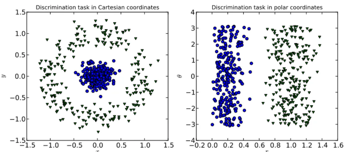
Figure 1.4 – Illustration of how changing representations can simplify a supervised learning problem. Here, a polar coordinates transform makes the problem linearly separable.

1.3 Neural Networks

1.3.1 Supervised learning

In supervised learning scenarios, specific representation of the input data em-ployed can have a profound impact on successful generalization. Much of the work involved in practical applications of machine learning amounts to the manual de-sign of features, deterministic functions of the raw input dede-signed such that the o↵-the-shelf supervised learning algorithm can easily interrogate the structure of the problem. In particular, methods based on a linear combination of input features such as logistic regression or the linear support vector machine (Cortes and Vapnik, 1995) have the desirable property that their loss functions are convex : importantly, there is one global minimum, and its approximate location can be determined by a variety of techniques from the convex optimization literature. In many real-world scenarios, however, linear decision boundaries are insufficiently flexible: a linear classifier cannot even learn the exclusive-OR function, as no linear decision bound-ary can be drawn between the examples corresponding to the “true” (1) output and the “false” output. Another example is shown in Figure 1.4, whereby a simple change of variables (to polar coordinates) makes an otherwise more challenging classification problem linearly separable in the new space.

(24)

trick” (Aizerman et al., 1964): the solution to the optimization of the support vector machine’s loss function is expressable in terms of inner products between training examples (Boser et al., 1992), and these inner products can be replaced with any kernel function satisfying mild conditions while retaining the convexity of the loss function. Kernel functions can be chosen such that they correspond to inner products in higher-dimensional spaces, or even infinite-dimensional Hilbert space, in which there exists a suitable linear decision boundary. It has been argued by Bengio and LeCun (2007) that the generalization capabilities of SVMs, especially when used in tandem with so-called “universal” kernels, is of a limited and local (in feature-space) character, and that richer mappings are necessary for nonlocal generalization. Kernelized SVMs are non-parametric in the sense that they depend on storing the support vectors, those training examples that lie on the margin adjacent to the decision boundary; for complicated classification problems this can lead to high computational complexity at test time, as well as a relatively large memory footprint.

Alternatively, multi-layer perceptrons (Rumelhart et al., 1986), also known as feed-forward neural networks o↵er a richer parametric approach, with one or more layers of nonlinear basis functions conventionally known as hidden units that are linearly combined in the output layer. For example, a multi-layer perceptron for binary classification with a single layer of hidden units could be parameterized as

h(x) = s(V x + c) (1.11)

o(x) = (wTh(x) + b) (1.12)

where V , w, c and b are learnable parameters, and s is some elementwise nonlinear-ity. The output of the hidden units h(x) is a learned, nonlinear transformation of the raw input, which can be adapted by gradient descent to the classification task at hand. Replacing (wTx + b) with o(x) in (1.3) and (1.5) gives us a more flexible extension of logistic regression that can be trained by gradient descent on the same loss function (1.5). Gradients on w and b are unchanged from standard logistic regression, while gradients on V and c (and, in general, the lower-layer parameters of any multilayer perceptron) are efficiently computable via the backpropagation al-gorithm (Rumelhart et al.,1986). Where simpler methods traditionally relied upon handcrafted features – fixed, hand-engineered transformations of the raw input –

(25)

neural networks o↵er the attractive possibility of learning to extract features using the hidden units of the network.

While such networks, even with a single layer of hidden units, are provably uni-versal approximators (Hornik et al.,1989) (i.e., with enough hidden units they can approximate, to an arbitrary degree of accuracy, any continuous function on com-pact subsets ofRn_{) this power comes at an additional cost. In gaining expressivity,} the convexity of the loss function is sacrificed; identification of a global optimum of the loss function is no longer guaranteed. While a single layer of hidden units may be sufficient to approximate any input-output mapping arbitrarily well, this may come at the cost of representational (and hence statistical) efficiency (see Bengio and LeCun (2007) for detailed arguments to this e↵ect). Multiple hidden layers can demonstrably lead to more efficient parameterizations (Bengio,2009), but con-ventional numerical optimizers, until recently, notoriously failed to e↵ectively train networks with more than one or two hidden layers (Glorot and Bengio,2010).

The recent wave of success in training deep neural networks is attributable to several factors. Recent work has yielded a better understanding of factors such as initialization and gradient acceleration methods (Sutskever et al.,2013) which play a crucial role in optimization. Recent years have seen the replacement of sigmoidal nonlinearities (namely the logistic and hyperbolic tangent functions) with non-saturating nonlinearities; Jarrett et al.(2009) first investigated several rectification nonlinearities in convolutional object recognition architectures, focusing on the absolute value rectification, whileNair and Hinton(2010) showed that the half-wave rectifier max(0, x), which they dubbed the Rectified Linear Unit (ReLU), could be fruitfully applied within the context of restricted Boltzmann machines. Glorot et al. (2011) showed that rectified linear units could be used to train very deep multilayer perceptrons without need of sophisticated initializations based on unsupervised pre-training. Piecewise linear activation functions, including rectifiers, give rise to networks which are piecewise affine functions, through which gradient signal propagates much more readily (see chapter 3 for an extended exploration of this topic). Finally, the availability of large amounts of data, and the use of commodity graphics processing units for the rapid training of these computationally intensive networks (Raina et al., 2009) has allowed practitioners to identify regimes of high performance that were previously obscured by small sample sizes and prohibitive training times.

(26)

1.3.2 Encoding domain knowledge

We have thus far considered learning systems which operate on training cases which are arbitrary vectors in Rn _{and pay no heed to structured relationships} between elements of these vectors. However, many signals of interest are highly structured, with elements having a natural topology in space or in time. A 32_{⇥ 32} pixel RGB image can be represented as a vector in R3072 _{and processed by any} algorithm that is agnostic to the fact that it is dealing with pixels, but this neglects readily available domain knowledge about the structure of the problem. Just as machine learning practitioners often engineer discriminative features of the input based on domain knowledge, so can one infuse domain knowledge into learnable feature extraction systems.

One way of introducing domain knowledge in a neural network is by restricting the connectivity pattern, or receptive field, of individual hidden units. Another way is to force di↵erent hidden units, operating on di↵erent inputs, to share the same parameters – that is, to process di↵erent inputs in exactly the same fashion. Taken together, these strategies form the bedrock of the most successful class of neural networks to date.

Convolutional neural networks

In the case of images, it is reasonable to assume that primitive features useful for classification, such as edges or corners, will have a spatially local character. A layer of hidden units whose individual connectivity patterns tile the image with small, overlapping receptive fields will thus force the network to learn features which are localized in space; the early processing layers of the mammalian visual system are known to have a similar structure (Hubel and Wiesel,1959).

The locally-connected regime described above would grant each locally con-nected hidden unit its own, independent weights. However, a useful property of images is that semantics are often preserved across translations in space; a bird is still a bird no matter if it appears perched on a window sill or on a tree branch. One can thus gain statistical efficiency by replicating the same weights across all spatial locations, allowing the network to detect a given, spatially localized pattern no matter where it appears. It is straightforward to show that the gradient of the surrogate loss with respect to the shared weights of these spatially replicated units

(27)

is simply the sum of the gradients with respect to each of its instantiations. A spatially replicated linear transformation on local pixel neighbourhoods is precisely equivalent to a discrete, 2-dimensional convolutioni_{, a common primitive} in image processing algorithms. Convolutional neural networks (LeCun, 1989; Le-Cun et al., 1998) incorporate these insights by replacing multiplication by weight matrices in neural networks with a linear transformation based on 2-dimensional convolutions. More precisely, some subset of a image’s M input channels are con-volved with 2-dimensional filters, and the results summed together; this is repeated N times, yielding N outputs from a total of N _{⇥ M learnable 2-dimensional} fil-ters. For each pixel in each of the N output planes, a plane-specific scalar bias is added, and a nonlinearity is applied. The resulting planes are known as feature maps. Convolutional neural networks repeat this structure, often interleaved with a spatial decimation operation such as taking the average or maximum value in a given neighbourhood (average pooling or max pooling, respectively), though more recently simple subsampling has become a popular alternative (Springenberg et al., 2015). If a discrete convolution is immediately followed by a fixed subsampling, the composed operation can be computationally streamlined by never computing the outputs of the convolution which will be immediately discarded. The composed operation is often referred to as strided convolution.ii

Convolutional layers involve some subtleties with respect to the treatment of image borders, particularly when “transposing” the convolution for the computation of gradients. We refer the reader to Dumoulin and Visin (2016) for a thorough treatment of the subject as it applies to neural networks in practice.

1.3.3 Unsupervised learning

We now turn our attention to the problem of performing unsupervised learning using neural networks.

Most modern methods for unsupervised deep learning have a straightforward

i. Equivalent up to a horizontal and vertical reversal of the weights, which is inconsequential if these weights are being fit to data rather than given a priori.

ii. N.B.: While the gradient of a convolution is always expressible as another convolution with a di↵erent treatment of the image border, the gradient of this combined operation is not expressible as a convolution, but rather a spatial dilation via the insertion of zeros, followed by a convolution. This “strided convolution-transpose”, “fractionally strided convolution”, or “up-convolution” operation is often used in image generation architectures, such as those employed in

(28)

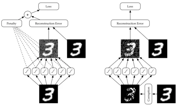
Reconstruction Error Reconstruction Error Penalty Co rr up tio n Loss Loss +

Figure 1.5 – A schematic diagram of a penalized autoencoder (left) and a denoising autoencoder (right).

interpretation in terms of probabilistic graphical models. While much of the early work on deep unsupervised learning relied heavily upon the machinery of undirected graphical models (Hinton et al., 2006; Hinton and Salakhutdinov, 2006; Salakhut-dinov and Hinton, 2009), more recent work bridging deep neural networks and probabilistic models has focused on directed latent variable models (Gregor et al., 2014; Mnih and Gregor, 2014; Rezende et al., 2014; Kingma and Welling, 2014; Goodfellow et al.,2014;Dinh et al.,2016) and fully-observed, auto-regressive mod-els (Larochelle and Murray, 2011; Germain et al., 2015;Oord et al., 2016).

In the interest of conciseness, we review only the concepts necessary to elucidate the contributions of this thesis. We review the venerable autoencoder, a determin-istic model which nonetheless underpins many modern probabildetermin-istically oriented techniques, and the denoising autoencoder, which admits an unconventional prob-abilistic interpretation. We further discuss generative adversarial networks (Good-fellow et al.,2014) in chapter 8.

(29)

Autoencoders

An autoencoder is a deterministic feed-forward neural network, i.e. akin to a multilayer perceptron, that is trained to reproduce its input in the output layer (rather than predict some target or response value). A simple single-layer autoen-coder might be parameterized as an enautoen-coder function h and a deautoen-coder function g

h(x) = s(Wx + b) (1.13)

g(x) = t(Vx + c) (1.14)

where s and t are elementwise activation functions and trained such that g(h(x))u x using a loss function appropriate for the domain of the inputs (and activation functions). In the case real-valued inputs with an assumption of independent Gaus-sian noise, squared Euclidean distance (“mean squared error”) between the input and the output vector is a reasonable choice; in the case of pseudo-binary inputs in [0, 1]D _{and t(}_{·) = (·), a reasonable choice may be the cross-entropy (discussed} in 1.1) when treating the inputs and outputs as the parameters of independent Bernoulli distributions. Autoencoders are closely related to Principal Components Analysis, an unsupervised dimensionality reduction method (Jolli↵e,1986): in par-ticular, an autoencoder is equivalent to PCA when trained with mean squared error, a number of hidden units K less than the number of input dimensions D, and s and t equal to the identity function (Baldi and Hornik, 1989). The columns of W will span the same subspace as the first K principal components, but will not form an orthonormal set.

In early work, authors focused on the case of fewer hidden units than input variables (Bourlard and Kamp, 1988), and a single hidden layer – autoencoders with many layers of nonlinear hidden units were traditionally considered difficult to train, though layerwise pre-training with RBMs (Hinton and Salakhutdinov, 2006) and more sophisticated optimization strategies (Martens,2010) have yielded successes in training deep autoencoders with a “bottleneck”.

In modern approaches, the over-complete (more hidden units than input di-mensions) setting is often preferred, but additional constraints or penalties are necessary in order to prevent trivial solutions: with more hidden units than feature

(30)

dimensions, there may be arbitrarily many mappings that reconstruct the input perfectly but fail to capture any interesting structure.

Denoising autoencoders

Vincent et al. (2008) proposed an alternate method of constraining the repre-sentation: corrupt each training example according to some noise process, and train the denoising autoencoder to reconstruct the original example from its corrupted counterpart. The same work showed that stacking these modules yields perfor-mance competitive with deep belief networks (Hinton et al., 2006), while Vincent (2011) showed a theoretical connection between single hidden layer denoising au-toencoders (trained with a squared error loss) and restricted Boltzmann machines trained with an alternative to maximum likelihood called score matching (Hyv¨ari-nen, 2005). Bengio et al. (2013) expanded upon this connection, proposing an interpretation of denoising autoencoders as generative models. This interpretation applies to arbitrary architectures and any loss function interpretable as a negative log likelihood.

(31)

2

Prologue to First Article

2.1 Article Details

Maxout networks. Ian J. Goodfellow, David Warde-Farley, Mehdi Mirza, Aaron Courville, and Yoshua Bengio. Proceedings of the 30th International Con-ference on Machine Learning (ICML ’13), pp. 1319-1327.

Personal Contribution. Ian Goodfellow and I jointly undertook engineering work (wrapping of the cuda-convnet library for use with Theano) for the imple-mentation of the large scale experiments. I proposed and implemented many of the probative experiments in sections 6 through 8, and performed the majority of the benchmark experiments on CIFAR10/CIFAR100. I co-wrote the manuscript with the other authors.

2.2 Context

A turning point in the adoption of deep learning methods came in 2012, when a convolutional neural network won the ImageNet Large Scale Visual Recognition Challenge (Krizhevsky et al., 2012). Two important components in the design of this network were the use of rectified linear activations (Jarrett et al., 2009; Nair and Hinton, 2010; Glorot et al., 2011) and the dropout method (Hinton et al., 2012) for regularization. Observations that dropout regularization appeared to be most e↵ective when used in conjunction with rectified linear activations led to the question of whether other piece-wise affine parameterizations would o↵er yet greater synergy with dropout.

(32)

2.3 Contributions

Maxout units o↵er a novel alternative to traditional elementwise activations, removing the saturating property of rectified linear units. We show that networks of maxout units improve upon several important classification benchmarks, and conduct extensive experiments to explain the improved performance.

2.4 Recent Developments

As of this writing, the manuscript has accrued over 800 citations. Maxout units have been successfully leveraged in a variety of applications of neural networks, in-cluding automatic speech recognition (Swietojanski et al.,2014;Zhang et al.,2014), automated speaker verification (Variani et al.,2014), whale call detection (Smirnov, 2013), face recognition (Schro↵ et al.,2015), visual person reidentification (Li et al., 2014), house number transcription from photographs (Goodfellow et al.,2014), and brain tumour segmentation (Havaei et al.,2017).

(33)

3

Maxout Networks

3.1 Introduction

Dropout (Hinton et al., 2012) provides an inexpensive and simple means of both training a large ensemble of models that share parameters and approximately averaging together these models’ predictions. Dropout applied to multilayer per-ceptrons and deep convolutional networks has improved the state of the art on tasks ranging from audio classification to very large scale object recognition (Hin-ton et al., 2012; Krizhevsky et al., 2012). While dropout is known to work well in practice, it has not previously been demonstrated to actually perform model aver-aging for deep architectures i _{. Dropout is generally viewed as an indiscriminately} applicable tool that reliably yields a modest improvement in performance when applied to almost any model.

We argue that rather than using dropout as a slight performance enhancement applied to arbitrary models, the best performance may be obtained by directly de-signing a model that enhances dropout’s abilities as a model averaging technique. Training using dropout di↵ers significantly from previous approaches such as ordi-nary stochastic gradient descent. Dropout is most e↵ective when taking relatively large steps in parameter space. In this regime, each update can be seen as mak-ing a significant update to a di↵erent model on a di↵erent subset of the trainmak-ing set. The ideal operating regime for dropout is when the overall training procedure resembles training an ensemble with bagging under parameter sharing constraints. This di↵ers radically from the ideal stochastic gradient operating regime in which a single model makes steady progress via small steps. Another consideration is that dropout model averaging is only an approximation when applied to deep models. Explicitly designing models to minimize this approximation error may thus enhance dropout’s performance as well.

i. Between submission and publication of this paper, we have learned that Srivastava(2013) performed experiments on this subject similar to ours.

(34)

We propose a simple model that we call maxout that has beneficial character-istics both for optimization and model averaging with dropout. We use this model in conjunction with dropout to set the state of the art on four benchmark datasets

i _.

3.2 Review of dropout

Dropout is a technique that can be applied to deterministic feed-forward archi-tectures that predict an output y given input vector v. These archiarchi-tectures contain a series of hidden layers h =_{h(1)_{, . . . , h}(L)_{}. Dropout trains an ensemble of models} consisting of the set of all models that contain a subset of the variables in both v and h. The same set of parameters ✓ is used to parameterize a family of distri-butions p(y _{| v; ✓, µ) where µ 2 M is a binary mask determining which variables} to include in the model. On each presentation of a training example, we train a di↵erent sub-model by following the gradient of log p(y | v; ✓, µ) for a di↵erent randomly sampled µ. For many parameterizations of p (such as most multilayer perceptrons) the instantiation of di↵erent sub-models p(y | v; ✓, µ) can be obtained by elementwise multiplication of v and h with the mask µ. Dropout training is similar to bagging (Breiman, 1994), where many di↵erent models are trained on di↵erent subsets of the data. Dropout training di↵ers from bagging in that each model is trained for only one step and all of the models share parameters. For this training procedure to behave as if it is training an ensemble rather than a single model, each update must have a large e↵ect, so that it makes the sub-model induced by that µ fit the current input v well.

The functional form becomes important when it comes time for the ensem-ble to make a prediction by averaging together all the sub-models’ predictions. Most prior work on bagging averages with the arithmetic mean, but it is not obvious how to do so with the exponentially many models trained by dropout. Fortunately, some model families yield an inexpensive geometric mean. When p(y _{| v; ✓) = softmax(v}>_{W +b), the predictive distribution defined by renormalizing} the geometric mean of p(y _{| v; ✓, µ) over M is simply given by softmax(v}>_{W/2 + b).}

i. Code and hyperparameters available athttp://www-etud.iro.umontreal.ca/~goodfeli/ maxout.html

(35)

In other words, the average prediction of exponentially many sub-models can be computed simply by running the full model with the weights divided by 2. This result holds exactly in the case of a single layer softmax model. Previous work on dropout applies the same scheme in deeper architectures, such as multilayer per-ceptrons, where the W/2 method is only an approximation to the geometric mean. The approximation has not been characterized mathematically, but performs well in practice.

3.3 Description of maxout

The maxout model is simply a feed-forward achitecture, such as a multilayer perceptron or deep convolutional neural network, that uses a new type of activation function: the maxout unit. Given an input x_{2 R}d_{(x may be v, or may be a hidden} layer’s state), a maxout hidden layer implements the function

hi(x) = max j2[1,k]zij

where zij = x>W···ij+ bij, and W 2 Rd⇥m⇥k and b2 Rm⇥k are learned parameters. In a convolutional network, a maxout feature map can be constructed by taking the maximum across k affine feature maps (i.e., pool across channels, in addition spatial locations). When training with dropout, we perform the elementwise multiplication with the dropout mask immediately prior to the multiplication by the weights in all cases–we do not drop inputs to the max operator. A single maxout unit can be interpreted as making a piecewise linear approximation to an arbitrary convex function. Maxout networks learn not just the relationship between hidden units, but also the activation function of each hidden unit. See Fig. 3.1 for a graphical depiction of how this works.

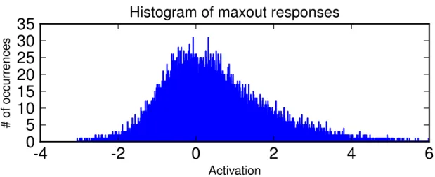
Maxout abandons many of the mainstays of traditional activation function de-sign. The representation it produces is not sparse at all (see Fig. 3.2), though the gradient is highly sparse and dropout will artificially sparsify the e↵ective rep-resentation during training. While maxout may learn to saturate on one side or the other this is a measure zero event (so it is almost never bounded from above). While a significant proportion of parameter space corresponds to the function being

(36)

x hi (x ) Rectifier x hi (x ) Absolute value x hi (x ) Quadratic

Figure 3.1 – Graphical depiction of how the maxout activation function can implement the rectified linear, absolute value rectifier, and approximate the quadratic activation function. This diagram is 2D and only shows how maxout behaves with a 1D input, but in multiple dimensions a maxout unit can approximate arbitrary convex functions.

bounded from below, maxout is not constrained to learn to be bounded at all. Max-out is locally linear almost everywhere, while many popular activation functions have signficant curvature. Given all of these departures from standard practice, it may seem surprising that maxout activation functions work at all, but we find that they are very robust and easy to train with dropout, and achieve excellent performance.

-4

-2

0

2

4

6

Activation

0

5

10

15

20

25

30

35

# of occu rr en ce s

Histogram of maxout responses

(37)

3.4 Maxout is a universal approximator

h

2 h

1 g

z

2,

_·

z

1,

_·

v

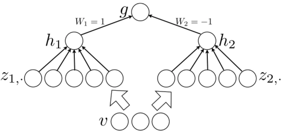
W1 = 1 W2= 1

Figure 3.3 – An MLP containing two maxout units can arbitrarily approximate any continuous function. The weights in the final layer can set g to be the di↵erence of h1 and h2. If z1 and z2

are allowed to have arbitrarily high cardinality, h1and h2can approximate any convex function.

g can thus approximate any continuous function due to being a di↵erence of approximations of arbitrary convex functions.

A standard MLP with enough hidden units is a universal approximator. Simi-larly, maxout networks are universal approximators. Provided that each individual maxout unit may have arbitrarily many affine components, we show that a maxout model with just two hidden units can approximate, arbitrarily well, any continuous function of v 2 Rn_{. A diagram illustrating the basic idea of the proof is presented} in Fig. 3.3.

Consider the continuous piecewise linear (PWL) function g(v) consisting of k locally affine regions on Rn_.

Proposition 3.4.1. (From Theorem 2.1 inWang(2004)) For any positive integers m and n, there exist two groups of n + 1-dimensional real-valued parameter vectors [W1j, b1j], j 2 [1, k] and [W2j, b2j], j 2 [1, k] such that:

g(v) = h1(v) h2(v) (3.1)

That is, any continuous PWL function can be expressed as a di↵erence of two convex PWL functions. The proof is given in Wang (2004).

Proposition 3.4.2. From the Stone-Weierstrass approximation theorem, let C be a compact domain C _{⇢ R}n_{, f : C} _{! R be a continuous function, and ✏ > 0 be any}

(38)

positive real number. Then there exists a continuous PWL function g, (depending upon ✏), such that for all v _{2 C, |f(v)} g(v)_{| < ✏.}

Theorem 3.4.3. Universal approximator theorem. Any continuous function f can be approximated arbitrarily well on a compact domain C ⇢ Rn_{by a maxout network} with two maxout hidden units.

Sketch of Proof By Proposition 3.4.2, any continuous function can be approxi-mated arbitrarily well (up to ✏), by a piecewise linear function. We now note that the representation of piecewise linear functions given in Proposition 3.4.1 exactly matches a maxout network with two hidden units h1(v) and h2(v), with sufficiently large k to achieve the desired degree of approximation ✏. Combining these, we conclude that a two hidden unit maxout network can approximate any continuous function f (v) arbitrarily well on the compact domain C. In general as ✏ _{! 0, we} have k_{! 1.}

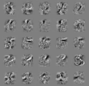
Figure 3.4 – Example filters learned by a maxout MLP trained with dropout on MNIST. Each row contains the filters whose responses are pooled to form a maxout unit.

(39)

Table 3.1 – Test set misclassification rates for the best methods on the permutation invariant MNIST dataset. Only methods that are regularized by modeling the input distribution outper-form the maxout MLP.

Method Test error Rectifier MLP + dropout (Srivastava, 2013) 1.05% DBM (Salakhutdinov and Hinton, 2009) 0.95% Maxout MLP + dropout 0.94% MP-DBM (Goodfellow et al., 2013) 0.88%

Deep Convex Network (Yu and Deng, 2011)

0.83%

Manifold Tangent Clas-sifier (Rifai et al., 2011)

0.81%

DBM + dropout (Hinton et al., 2012)

0.79%

3.5 Benchmark results

We evaluated the maxout model on four benchmark datasets and set the state of the art on all of them.

3.5.1 MNIST

The MNIST (LeCun et al., 1998) dataset consists of 28 ⇥ 28 pixel greyscale images of handwritten digits 0-9, with 60,000 training and 10,000 test examples. For the permutation invariant version of the MNIST task, only methods unaware of the 2D structure of the data are permitted. For this task, we trained a model consisting of two densely connected maxout layers followed by a softmax layer. We regularized the model with dropout and by imposing a constraint on the norm of each weight vector, as in (Srebro and Shraibman, 2005). Apart from the maxout units, this is the same architecture used by Hinton et al. (2012). We selected the hyperparameters by minimizing the error on a validation set consisting of the last 10,000 training examples. To make use of the full training set, we recorded the

(40)

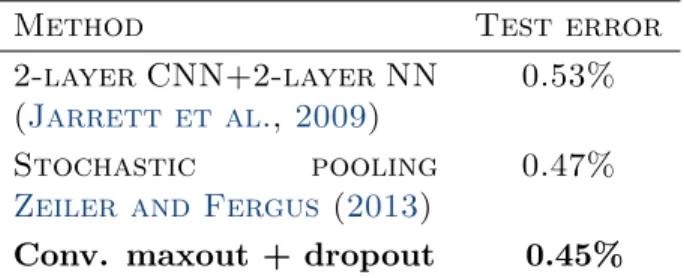
Table 3.2 – Test set misclassification rates for the best methods on the general MNIST dataset, excluding methods that augment the training data.

Method Test error 2-layer CNN+2-layer NN

(Jarrett et al., 2009)

0.53%

Stochastic pooling

Zeiler and Fergus (2013)

0.47%

Conv. maxout + dropout 0.45%

value of the log likelihood on the first 50,000 examples at the point of minimal validation error. We then continued training on the full 60,000 example training set until the validation set log likelihood matched this number. We obtained a test set error of 0.94%, which is the best result we are aware of that does not use unsupervised pretraining. We summarize the best published results on permutation invariant MNIST in Table 3.1.

We also considered the MNIST dataset without the permutation invariance restriction. In this case, we used three convolutional maxout hidden layers (with spatial max pooling on top of the maxout layers) followed by a densely connected softmax layer. We were able to rapidly explore hyperparameter space thanks to the extremely fast GPU convolution library developed by Krizhevsky et al.(2012). We obtained a test set error rate of 0.45%, which sets a new state of the art in this category. (It is possible to get better results on MNIST by augmenting the dataset with transformations of the standard set of images (Ciresan et al., 2010).) A summary of the best methods on the general MNIST dataset is provided in Table 3.2.

3.5.2 CIFAR-10

The CIFAR-10 dataset (Krizhevsky and Hinton,2009) consists of 32 _{⇥ 32 color} images drawn from 10 classes split into 50,000 train and 10,000 test images. We preprocess the data using global contrast normalization and ZCA whitening.

We follow a similar procedure as with the MNIST dataset, with one change. On MNIST, we find the best number of training epochs in terms of validation set error, then record the training set log likelihood and continue training using the entire training set until the validation set log likelihood has reached this value. On

(41)

Table 3.3 – Test set misclassification rates for the best methods on the CIFAR-10 dataset.

Method Test error Stochastic pooling

Zeiler and Fergus (2013)

15.13%

CNN + Spearmint Snoek et al. (2012)

14.98%

Conv. maxout + dropout 11.68 % CNN + Spearmint +

data augmentation Snoek et al. (2012)

9.50 %

Conv. maxout + dropout + data augmentation

9.38 %

CIFAR-10, continuing training in this fashion is infeasible because the final value of the learning rate is very small and the validation set error is very high. Training until the validation set likelihood matches the cross-validated value of the training likelihood would thus take prohibitively long. Instead, we retrain the model from scratch, and stop when the new likelihood matches the old one.

Our best model consists of three convolutional maxout layers, a fully connected maxout layer, and a fully connected softmax layer. Using this approach we obtain a test set error of 11.68%, which improves upon the state of the art by over two percentage points. (If we do not train on the validation set, we obtain a test set error of 13.2%, which also improves over the previous state of the art.) If we additionally augment the data with translations and horizontal reflections, we obtain the absolute state of the art on this task at 9.35% error. In this case, the likelihood during the retrain never reaches the likelihood from the validation run, so we retrain for the same number of epochs as the validation run. A summary of the best CIFAR-10 methods is provided in Table 3.3.

3.5.3 CIFAR-100

The CIFAR-100 (Krizhevsky and Hinton, 2009) dataset is the same size and format as the CIFAR-10 dataset, but contains 100 classes, with only one tenth as many labeled examples per class. Due to lack of time we did not extensively

Feedforward deep architectures for classification and synthesis

Résumé

Summary

Contents

List of Figures

List of Tables

List of Abbreviations

Acknowledgments

1

Background

1.0.1

Parametric and non-parametric learning

1.0.2

Parameters and hyperparameters

1.1

Formalizing learning

1.2

Probabilistic graphical models

a

b

c

d

e

f

1.2.1

Directed models and explaining away

1.3

Neural Networks

1.3.1

Supervised learning

1.3.2

Encoding domain knowledge

1.3.3

Unsupervised learning

2

Prologue to First Article

2.1

Article Details

2.2

Context

2.3

Contributions

2.4

Recent Developments

3

Maxout Networks

3.1

Introduction

3.2

Review of dropout

3.3

Description of maxout

-4

-2

0

2

4

6

0

5

10

15

20

25

30

35

Histogram of maxout responses

3.4

Maxout is a universal approximator

h

2

h

1

g

z

2,

·

z

1,

·

_·

_·