EFFICIENT GENERATION OF THE IDEALS OF A POSET
IN GRAY CODE ORDER
THÈSE
PRÉSENTÉE
COMME EXIGENCE PARTIELLE
DU DOCTORAT EN MATHÉMATIQUES
PAR
MOHAMED AB DO
EFFICIENT GENERATION OF THE IDEALS OF A POSET
IN GRAY CODE ORDER
THESIS
PRESENTED
IN PARTIAL SATISFACTION OF THE REQUIREMENTS
OF THE DEGREE OF DOCTOR OF PHILOSOPHY IN MATHEMATICS
BY
MOHAMED ABDO
Avertissement
La diffusion de cette thèse se fait dans le respect des droits de son auteur, qui a signé le formulaire Autorisation de reproduire et de diffuser un travail de recherche de cycles supérieurs (SDU-522 - Rév.01-2006). Cette autorisation stipule que «conformément à l'article 11 du Règlement no 8 des études de cycles supérieurs, [l'auteur] concède à l'Université du Québec à Montréal une licence non exclusive d'utilisation et de publication de la totalité ou d'une partie importante de [son] travail de recherche pour des fins pédagogiques et non commerciales. Plus précisément, [l'auteur] autorise l'Université du Québec à Montréal
à
reproduire, diffuser, prêter, distribuer ou vendre des copies de [son] travail de recherche à des fins non commerciales sur quelque support que ce soit, y compris l'Internet. Cette licence et cette autorisation n'entraînent pas une renonciation de [la] part [de l'auteur] à [ses] droits moraux ni à [ses] droits de propriété intellectuelle. Sauf entente contraire, [l'auteur] conserve la liberté de diffuser et de commercialiser ou non ce travail dont [il] possède un exemplaire.»1 would like to thank Timothy Walsh, director of my research, for what he taught me, for his encouragement, for the time he spent answering my questions, for his valu able advice given to me when 1 was a teaching assistant for his course, and for his financial support. Without his supervision, this work would not have been completed. ln addition, 1 thank him for the concerts to which he invited me when he was celebrating his birthday and elsewhere.
1 would also like to thank Srecko Brlek for what he taught me and for his interest in students and especially for his valuable advice, encouragement and collaboration.
1 thank my father Abdulhamid and my mother Naima who supported and con stantly encouraged me to achieve my dreams in my studies.
1 will never forget my brother Ahmad who passed away in November 2009. He was my real friend and support, we were as twins.
l'm glad that my wife was beside me while 1 was writing my thesis. 1 owe her a lot because she gives me the love and enthusiasm that 1 need.
Thanks to Manon Gauthier, who provides ail the administrative advice and who shows much interest in students. Thanks to Gisèle Legault, who, with her knowledge of computers, allowed me to save much time. Thanks to Lise Tourigny, Jérôme Tremblay and ail the staff in the Departments of Mathematics and Computer Science.
Finally, 1 am grateful to LaCIM, ISM, FARE, FQRNT and the Faculty of Sciences for their financial support during my studies for my M.Sc. and Ph.D. These scholarships were complementary to the financial support of my supervisor.
LIST OF FIGURES IX RÉSUMÉ . . Xlii CHAPTER l LIST OF TABLES XI ABSTRACT XV INTRODUCTION 1 GRAY CODE 5 1.1 Introduction. 5
1.2 Construction of a Hamiltonian cycle 8
1.3 Hamiltonian cycle when the median is a minimal element 9 1.4 Hamiltonian cycle when there is exactly one element less than the median 13 1.5 Generalization of Squire's recurrence . . . 16 1.6 Hamiltonian cycle using our generalization of Squire's recurrence 17 1.7 Hamiltonian cycle when there are at least two elements less than the median 23 CHAPTER II
ALGORITHMS 35
2.1 Representation and useful functions 35
2.2 Printing ideals . 36
2.2.1 Order of printing the ideals when applying Theorem 1 36
2.2.2 Order of printing the ideals when applying Theorem 2 37 2.2.3 Order of printing the ideals when applying Theorem 3 38
2.3 Use of Lemma 1 and Lemma 2 38
2.4 Algorithms . 38
2.5 How to choose the median element 46
2.5.1 Relaxed condition . . . 46
2.5.3 Choosing the median for Theorem 2 49
2.5.4 Choosing the median for Theorem 3 49
CHAPTER III
COMPARISON OF ALGORITHMS 53
3.1 Boolean lattice family 56
3.2 Grid poset family . . 57
3.3 Gamma poset family 58
3.4 Linear posets 58 3.5 Empty posets 59 CONCLUSION 65 APPENDIX A PROGRAMS 67 Al Our Program 67
A.2 Ruskey's program 101
A.3 Our implementation of Squire's algorithm 107
A.4 Data entering program . 112
1.1 Poset of Example 1 is on the left side. . . . . 8
1.2 Left side is the poset having x as a minimal element. 10
1.3 Cycle of Case 1 of Theorem 1.. 10
1.4 Cycle of Case 2 of Theorem 1.. 11
1.5 Exam pie ill ustrating the use of Theorem l, Case 2. 12
1.6 Example illustrating the use of Theorem 1, Case 1. 12
1.7 First case of Theorem 2. . . 14
1.8 Second case of Theorem 2.. 15
1.9 Example illustrating the use of Theorem 2. 16
1.10. Illustration of Lemma 1. . 18
1.11. Example illustrating the use of Lemma 1. 19
1.12. III ustration of Lemma 2. Lines 2-3 cover Case 1, !ines 4-5 cover Case 2 and lines 6-7 cover Case 3. . . .. 20
1.13. Example illustrating the use of Lemma 2. 23
1.14. First case of the basic step in Lemma 3. . 24
1.15. Second case of the basic step in Lemma 3. 25
1.17. First subcase of first case in Theorem 3. . 30 1.18. Second subcase of first case in Theorem 3. 30
1.19. Second case of Theorem 3 . 31
1.20. Example illustrating the use of Theorems 1 and 3 as well as Lemma 1. 33
2.1 Algorithm coding Theorem 1. 40
2.2 Algorithm coding Theorem 2. 41
2.3 Algorithm coding Theorem 3. 42
2.4 Our algorithm for generating the ideals of a poset. 42
2.5 Algorithm coding Lemma 1. 43
2.6 Algorithm coding Lemma 2. 44
2.7 Pruesse and Ruskey's algorithm for generating a Gray code for the ideals of a poset. . . . . . 45
2.8 Squire's algorithm for generating the ideais of a poset. 46
2.9 Choosing X m for the median element in a linear extension of P.
47
2.10. Left si de is the poset having x as a minimal element. . . . 48
2.11. Example illustrating the use of Theorem 1 with the relaxed condition. QO
2.12. Example illustrating the use of Theorem 3 and Theorem 1 with the relaxed condition. . . . .. 52
3.1 Boolean lattice of 8 elements. 56
3.2 Grid poset of 8 elements. 57
3.1 Running times of the programs for poset1. 54
3.2 Running times of the programs for poset2. 55
3.3 Running times of the programs for poset3. 55
3.4 Running times of the programs for poset4. 55
3.5 Running timc of execution on a family of boolean lattices. 61 3.6 For boolean lattices, our progTam is 4.7% on the average slower than
Squire's and Ruskey's is 9.6% slower than Squire's. . . .. 61
3.7 Running time of execution on a family of grid posets.. 61
3.8 For grid posets, our program is 1.9% on the average slower than Squire's and Ruskey's is 25.4% slower than Squire's. . . .. 62
3.9 . Running time of execution on a family of gamma posets. 62
.3.10. For gamma posets, our program is 1.7% on the average slower than Squire's and Ruskey's is 1.8% slower than Squire's. . . .. 62 3.11. Running time of execution on a family of linear posets.. 63 3.12. For linear posets, our program is 2.1% on the average slower than
Squire's and Ruskey's is 37.7% slower than Squire's. . . .. 63
3.13. Running time of execution on a family of empty posets. 63
3.14. For empty posets, our program is 2.3% on the average slower than Squire's and Ruskey's is 1.9% slower than Squire's. . . .. 64
Pruesse et Ruskey ont présenté un algorithme pour la génération de leur code Gray pour les idéaux d'un poset (ensemble partiellement ordonné) où deux idéaux adjacents diffèrent par un ou deux éléments. Leur algorithme fonctionne en temps amorti de O(n) par idéal. Squire a présenté une récurrence pour les idéaux d'un poset qui lui a permis de trouver un algorithme pour générer ces idéaux en temps amorti de O(logn) par idéal, mais pas en code Gray. Nous utilisons la récurrence de Squire pour trouver un code Gray pour les idéaux d'un poset, Ol! deux idéaux adjacents diffèrent par un ou deux éléments. Dans le pire des cas, notre algorithme a la même complexité que celle de l'algorithme de Pruesse et Ruskey et dans les autres cas, sa complexité est meilleure que celle de leur algorithme et se rapproche de celle de l'algorithme de Squire. Squire a donné une condition pour obtenir cette complexité. Nous avons trouvé une condition moins restrictive que la sienne. Cette condition nous a permis d'améliorer la complexité de notre algorithme.
Mots clés: poset, extension linéaire, cycle hamiltonien, code Gray, algorithme, complexité.
Pruesse and Ruskey presented an algorithm for generating their Gray code for the ideals of a poset, where two adjacent ideals differ by one or two elements. Theil' algorithm takes O(n) amortized time pel' ideal, where n is the number of elements in the poset. Squire presented a recurrence for the ideals of a poset that enabled him to find an algorithm for generating these ideals in O(log n) amortized time pel' ideal, but not in Gray code order, where n is the number of elements in the poset. We use Squire's recurrence to find a Gray code for the ideals of a poset, where two adjacent ideals differ by one or two elements. In the worst case our algorithm has the same complexity as that of Pruesse and Ruskey and in the other cases its complexity is better and approaches that of Squire's algorithm. Squire gave a condition to obtain this complexity. We found a less restrictive condition than his. This condition enabled us to improve the complexity of our algorithm.
Key words: poset, linear extension, Hamiltonian cycle, Gray code, algorithm,
"Humanity has long enjoyed making lists. Ali children delight in their new-found ability to count 1,2,3, etc., and it is a profound revelation that this pro cess can be carried out indefinitely. The fascination of finding the next unknown prime or of listing the digits of
7r appeals to the general population, not just mathematicians. The desire to produce
lists almost seems to be an innate part of our nature. Furthermore, the solution to many problerns begins by listing the possibilities that can arise" (Ruskey,2003). It was not until 1960 that generation of such combinatoriallists would be feasible with the advent of the computer (Lehmer, 64). However, for such a listing to be possible, generation methods must be efficient. A common approach has been to try to generate such lists so that successive objects differ by sorne predefined small amount. A famous example is the binary refiected Gray code (Gilbert, 58; Gray, 53) which consists of listing aIl the binary numbers of the same size so that successive numbers differ in exactly one bit.
The origins of listing combinatorial objects so that successive objects differ only by small amount can be found in the early work of (Gray, 53; Wells, 61; Trotter, 62; Johnson, 63; Lehmer, 65; Chase, 70; Ehrlich, 73; Nijenhuis and Wilf, 78). However, the term combinatoriaJ Gray code first appeared in (Joichi, White and Williamson, 80).
There are many combinatorial Gray codes such as:
1. listing ail the permutations of 1,2, ... , n so that successive permutations differ only by the swap of one pair of adjacent elements (Johnson, 63; Trotter, 62);
2. listing ail the k-element subsets of an n-element set in such a way that successive sets differ by exactly one element (Bitner, Ehrlich and Reingold, 76; Buck and
Wiedemann, 84; Eades, Hickey, and Read, 84; Eades and McKay, 84; Nijenhuis and Wilf, 78; Ruskey, 88; Liu and Tang, 73);
3. listing aU the partitions of an integer n so that in successive partitions, one part has increased by one and one part has decreased by one (Savage, 89);
4. listing the linear extensions of certain posets so that successive elements differ only by a transposition (Ruskey, 92; Pruesse and Ruskey, 91; Stachowiak, 92; West, 93);
5. listing aU the binary trees of a given size so that consecutive trees differ only by a rotation at a single node (Lucas, 87; Lucas, Roelants and Ruskey, 93; Proskurowski and Ruskey, 90);
6. listing the well-formed parenthesis strings of a given length in such a way that suc cessive strings differ by a transposition of two letters (PrQskurowski and Ruskey, 90). Walsh is the first who gave a loop-free generation algorithm for this problem
(Walsh, 98);
7. listing aU the length-n involutions so that each involution is transformed into its successor via one or two transpositions or a rotation of three elements (Walsh, 2001).
8. listing all the ideals of a poset so that successive ideals differ in one or two elements (Abdo, 2009; Pruesse and Ruskey, 93; Koda and Ruskey, 93).
This thesis presents another Gray code for the ideals of a poset and an algorithm for generating these ideals that runs as least as fast as that of (Pruesse and Ruskey, 93) on aU the posets on which we tested it and considerably faster on some of them. The definition of a poset and of an ideal, an outline of the thesis and a summary of the major results appear in the first two pages of Chapter 1.
One can find applications of the Gray code to circuit design (Robinson and Cohn, 81), signal processing (Ludman, 81), ordering of documents on shelves (Losee, 92), data
compression (Richard, 86), statistical computing (Diaconis and Bolmes, 94), combina torial map theory (Cori, 75), graphies and image processing (Amalraj, Sundararajan and Dhar, 90), processor allocation in the hypercube (Chen and Shin, 90), hashing (Faloutsos, 88), computing the permanent (Nijenhuis and Wilf, 78), information stor age and retrieval (Chang, Chen and Chen, 92), and puzzles, such as the Chinese Rings and Towers of Banoi (Gardner, 72).
"Although many Gray code schemes seem to require strategies tailored to the problem at hand, a few general techniques and unifying structures have emerged. The paper (Joichi, White and Williamson, 80) considers families of combinatorial objects, whose size is defined by a recurrence of a particular form, and some general results are obtained about constructing Gray codes for these families. Ruskey shows in (Ruskey, 92) that certain Gray code listing problems can be viewed as special cases of the problem of listing the linear extensions of an associated poset so that successive extensions differ by a transposition. In the other direction, the discovery of a Gray code frequently gives new insight into the structure of the combinatorial class involved" (Savage, 97).
Walsh generalized Chase's method (Chase, 89) so that ail the words in a suffix-partitioned list form an interval of consecutive words ('Walsh, 95). Moreover, he gave sufficient con ditions on a Gray code in order that Ehrlich's method (Ehrlich, 73) possesses a loop-free implementation and he generalized this method so that it works under less restrictive conditions (Walsh, 2000).
"So, the area of combinatorial Gray codes includes many questions of interest in combi natorics, graph theory, group theory, and computing, including some well-known open problems" (Savage, 97).
GRAY CODE
1.1
Introduction
A paset (partiaUy ordered set) P is a set E of elements together with a reflexive, transitive, anti-symmetric relation R(P) on E. An up-set of a poset P is a subset U of
E such that if xE U and y 2 x, then YEU. A dawn-set of a poset P is a subset D of E such that if x E D and y ::::; x, then y E D. The set of ideals of a poset is either the set of aH its up-sets or the set of aU its down-sets. Generating the ideals of a poset has severaI applications in optimization problems, including scheduling, reliability and line balancing problems (Steiner, 86). Schrage and Baker (Schrage and Baker, 78), Lawler (Lawler, 79), and BaH and Provan (BaH and Provan, 83) aIl presented algorithms that generate the set U(P) of up-sets of Pin O(n2·u(P)) time, where u(P) is the cardinality of U(P). Steiner (Steiner, 86) was the first to present an O(n·u(P)) generation algorithm. Squire (Squire) presented a recurrence for the ideals of a poset and used it to generate these ideals in O(logn . u(P)) time. But none of these algorithms, including that of Squire, generates them in Gray cade arder - that is, so that two adjacent ideals in the list differ by a bounded number of elements. The advantage of Gray code order is that certain properties of the members of a list can be updated quickly if adjacent members of a list differ only slightly.
If the Hasse diagram of the poset
P
is a forest, the algorithms of Beyer and Ruskey (con stant average time generation of subtrees of bounded size, 1989, unpublished manuscript),and Koda and Ruskey (Koda and Ruskey, 93) can generate its up-sets in Gray code order in O(u(P)) time. Another class of posets for which an efficiently implementable Gray code exists is presented in (Knuth and Ruskey, 2003). However, for arbitrary posets, the best known algorithms, including that of Pruesse and Ruskey (Pruesse and Ruskey, 93), may still take 0(.6. . u(P)) time, where .6. is the maximum number of ele ments that cover any element of
P.
Their algorithm generates a list of the ideals of a poset so that two ideals that are adjacent in the list differ by one or two elements. We say that an element v covers an element t if t<
v and there is no element u such thatt <
u<
v. When v coverst,
we say thatt
is covered by v.In this thesis an ideal will mean a down-set. We generalize Squire's recurrence and use our generalized recurrence to list the elements of D(P), the down-sets of P, so that two ideals that are adjacent in the list differ by one or two elements, as does the algorithm of Pruesse and Ruskey (Pruesse and Ruskey, 93). A preliminary version of our algorithm, described in Section 1.3 and published in (Abdo, 2009), is similar to the one in (Pruesse and Ruskey, 93) except that it lists each ideal once instead of twice. The presentation here is simpler than the one in (Pruesse and Ruskey, 93) because it deals only with posets, whereas the one in (Pruesse and Ruskey, 93) is generalized to antimatroids. We were recently informed that the proof in (Pruesse and Ruskey, 93) was recast in terms of posets in Theorem 4.4 (Chow and Ruskey, 09), published in the same year as (Abdo, 2009). Both algorithms have the same time-complexity. However, we were able to improve the time-complexity of our algorithm so that it never ran more than a few percent slower than Squire's on any of the posets on which we tested it, whereas the Pruesse-Ruskey algorithm ran considerably slower on sorne of them.
The theory behind our algorithm is presented in Chapter 1, the algorithm itself in Chap ter 2, the experimental comparison of our algorithm with the Pruesse-Ruskey algorithm and the Squire algorithm in Chapter 3 and the source code of al! three algorithms in the Appendix A.
tension of P. If the number of elements of P is n then the position of the median is
l
nt
lJ.
We introduce the following notation that will be used in equation (1.1) below. Let P be a poset on a set E, D a down-set of P and Y a subset of E such that D
n
Y=
o
and D U Y is a down-set of P. Also, denote by D(P, D, Y) the set {I E D(P) : Dç
land lç
Du Y} of down-sets of P that contain the down-set D and whose other elements are chosen from Y. Finally, let x be some element of Y and D[x] and U[x] be, respectively, the elements of P that are:::; x and2:
x. Note that D(P) = D(P,0,
E). Squire's recurrence for the down-sets is given by equation (1.1):D(P, D, Y)
=
D(P, D, Y \ U[x]) U D(P, Du D[x], Y \ D[x]). (1.1) This recurrence is solvable because #(Y \ U[x]) and #(Y \ D[x]) are both strictly less than #(Y), where #(S) means the cardinality of the set S, and D(P, D, 0) = D.This recurrence is called initially with D
=
0
and Y=
E to generate D(P). In what follows we cali D(P, D, Y \ U[x]) the first part and D(P, Du D[x], Y \ D[x]) the second part. These two parts are disjoint. Usually we consider D(P, D, Y\D[x]) as the second part and then we add D[x] to each ideal of this part. Squire's method of generating the ideals of Pin O(logn· u(P)) time depends upon choosing for x the "median" element of Y in the following sense. An extension of a poset P on a setE
is a poset Q on E such that R(P)ç
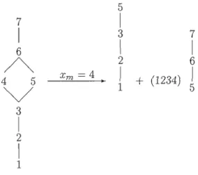
R( Q). An extension of P that is a total order is called a linear extension of P. Before calling the recurrence (1.1), Squire constructs a linear extension of P. The elements of Y are then listed in the order that is compatible with that of the linear extension, and the median element Xm in this list is chosen for x. We illustrate the use of (1.1) in the following example.Example 1. Let P be the poset whose Hasse diagram is on the left side (of the arrow) in Figure 1.1. In equation
(l.l),
let D be the empty down-set (/) andY
be the set{1, 2, ... , 7}. The linear extension chosen for P is 1
<
2<
3<
4<
5<
6<
7 so that the median element Xm is4.
The diagram immediately to the right of the arrow5
7 1 1 3 7 6 1 1A
4V
5 X m=
4. 2l
+
(1234) 6~
3 1 2 1 1Figure 1.1. Poset of Example 1 is on the left side.
is the poset restricted to Y \ U[4] and the rightmost diagram is the poset restricted
to Y \ D[4] with D[4] (with the commas removed and the braces replaced by brackets)
written to its left. The set of ail the dawn-sets of P is the union of two disjoint sets (parts). The first part is the set of dawn-sets whose elements are restricted to the set y \ U[4]
=
{l, 2, 3, 5}
and the second part is the set of down-sets that contain all of the elements of D[4] ={1, 2, 3, 4}
and whose other elements are restricted to the set y \ D[4]=
{5, 6, 7}.
Each of these parts can then he partitioned into two parts and sa on until all the parts contain at most two down-sets (corresponding ta Y which contains at most one element).1.2
Construction of a Hamiltonian cycle
A Hamiltonian cycle in a graph is a cycle that passes through each vertex exactly once. Given a poset P, we call G(P) the graph whose vertices are the down-sets of P, where two vertices are adjacent (joined by an edge) if the corresponding down-sets differ by one element and G2 (P) the graph with the same vertex set as G(P) but which has an edge between every pair of vertices that are connected by a path of length at most 2 in G(P). We use Squire's recurrence to construct a Hamiltonian cycle in G2(P), so that
two adjacent down-sets, as well as the first and last ones, differ by one or two elements. In what follows, when we refer to a Hamiltonian cycle in P, we mean a Hamiltonian
cycle in G2(P).
In our construction, the basic step is to caU a single vertex and a single edge (traversed in both directions) a Hamiltonian cycle, so that a single down-set or a pair of down-sets that differ by at most two elements constitutes a Hamiltonian cycle. For the induction step we assume that a Hamiltonian cycle has been found for the first part V(P, D,
y \
U[x]) of (1.1) and also for the second part V(P, Du D[x], Y \ D[x]) of (1.1) and we merge these two Hamiltonian cycles into a single one for V(P, D, Y).1.3 Hamiltonian cycle when the median is a minimal element
Theorem 1 below (Abdo, 2009) shows that a Hamiltonian cycle can be constructed for any poset. We cali x a maximal (minimal) element of a poset P if no element of P is strictly greater (less) than x. When a poset has only one maximal (minimal) element, this element is called maximum (minimum). We note that any finite poset must contain at least one maximal element and one minimal element.
Theorem 1. Let P be a poset on a set E and let x be a minimal element of P. Then there is a Hamiltanian cycle of dawn-sets in P in which twa adjacent dawn-sets differ by one or two elements and this cycle contains the edge
{0,
{x}} consisting of the empty down-set and the singleton {x}.Proof. (By induction on n = #(E), the cardinality of E).
Basic step. If n = 1, then the poset consists of a single element x, which is necessarily a minimal element, and has two ideals
0
and{x},
which differ by a single element. Then the edge{0,
{x}}
is the required Hamiltonian cycle.Induction step. Suppose that n
>
1. We apply (1.1) with the initial valuesD
=
0
and Y=
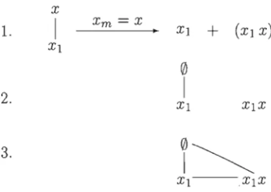
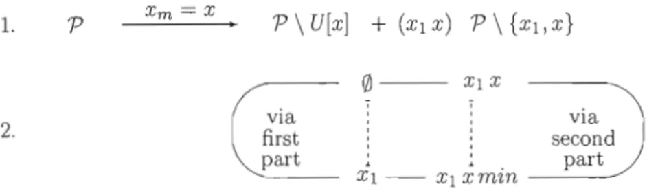
E and with x a minimal element of Y. Since x is a minimal element of Y, every element of Y is either in U[x] or else is incomparable with x. Then P, restricted to Y, is the poset on the left side of Figure 1.2. Since D[x] = {x}, the poset of the first partxm = x
P
P\U[x]
+
(x)
P \
{x}
Figure 1.2. Left side is the poset having x as a minimal element.
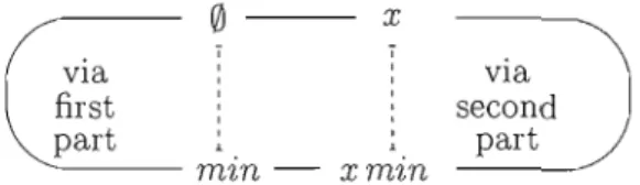
0 - -
xvia via
first second
part part
"'---- m'tn -
x
m~nFigure 1.3. Cycle of Case 1 of Theorem 1.
of (1.1) (restricted to Y \
U[x])
consists ofP \
U[x]
and the poset of the second part (restricted to Y \D[x]
=
Y \{x})
is of the form shown to the right of the+
sign in Figure 1.2. There are two cases to consider, depending upon whether or not Y \U[x]
is empty.
Case 1: Suppose that Y \
U[x]
=f
0.
Letmin
be a minimal element of Y \U[x].
Sincex
tf-
y \U[x], #(Y \ U[x])
<
#(E),
so that by the induction hypothesis there is a Hamiltonian cycle of down-sets of the first part in which two adjacent down-sets differ by one or two elements and this cycle contains the edge{0,
{min} }.
The second part is restricted to the set Y \{x},
which is not empty becausen
>
1 and whose cardinality<
#(E)
because it does not containx.
In addition, Y \{x}
hasmin
as minimalelement. It follows from the induction hypothesis that this part too has a Hamiltonian cycle of down-sets in which two adjacent down-sets differ by one or two elements and that this cycle too contains the edge
{0,
{min} }.
Whenx
is added to each ideal of this second cycle, this cycle will contain the edge{{x}, {x, min} }.
By removing the edges{0,
{min}}
and{{x}, {x, min}}
and adding the edges{0,
{x}}
and{{min}, {x, min}}
o
xvia second
~
partxmin
Figure 1.4. Cycle of Case 2 of Theorem 1.
Case 2: Suppose that Y \ U[x]
= 0.
Let min be a minimal element of Y \ D[x]. Such an element exists because Y \{x}
f.
0 sincen
>
1. The first part of (1.1) consists of the single down-set0.
By an argument similar to that in Case 1, the second part of (1.1) has a Hamiltonian cycle containing the edge{0,
{min}}, which becomes {{x}, {x, min}} when x is added to each down-set. By removing the edge {{x}, {x, min}} and adding the edges{0,
{x} } and{0,
{x, min}} we obtain the required Hamiltonian cycle contain ing the edge{0, {x}}
(see Figure 1.4). 0To simplify the notation, the set
{Xl,
X2,' .. ,xn } will be denoted by XIX2 ... xn ·Remark 1. We remove an edge from a cycle only when this cycle is not an edge or if
it is an edge and each of its vertices will be joined by an edge with two other vertices.
Example 2. Consider the poset on the left side of the first line of Figure 1.5. Ey c(wosing 1 for the minimal element X m and applying Theorem 1, Case '2, we obtain the first line of Figure 1.5. The first part is the empty poset which has the Hamiltonian
cycle 0. The second part is the poset 2 which has the Hamiltonian cycle {0,2}. Ey
adding the element 1 to each ideal of this last cycle we obtain the Hamiltonian cycle
{1,12}. Sinee we applied Theorem l, Case 2, we add the edges {0, 1} and {0,12} but
according to Remark 1, we do not remove the edge {1, 12}. Thus, we obtain the required
Hamiltonian cycle
{0,
1, 12} which is on the second line of Figure 1.5. We note thatthis cycle contains the edge {ŒI, 1}.
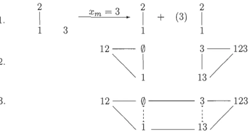
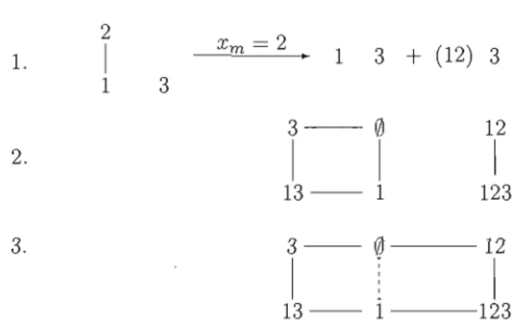
Example 3. Consider the poset on the left side of the first line of Figure 1.6. Ey choosing 3 for the minimal element X m and applying Theorem 1, Case 1, we obtain the
2
X m
=
1 ,0
+
(1) 21. 1
1 2.
Figure 1.5. Example illustrating the use of Theorem 1, Case 2.
2 2 2 Xm
=
3 ,+
(3) 1. 1 1 1 1 3 1 1 1 2 - - 0 3--123 2.~!
1 1 3 / 3. 1 2 - - 0 3--123~l
1~/
Figure 1.6. Example illustrating the use of Theorem 1, Case 1.
first line of Figure 1.6. Each of the first and the second parts is the poset
{1, 2}
where1
<
2 which, according to Example 2, has the Hamiltonian cycle {0, 1, 12}. By adding the element 3 to each ideal of the cycle of the second part we obtain the H amiltoniancycle {3, 13, 123}. The cycle of each part is on the second line of Figure 1.6. Since we applied Theorem 1, Case 1, we add the edges {0,3} and {1, 13} and remove the edges
{0,1} and {3, 13}. Thus, we obtain the required Hamiltonian cycle on the third line of Figure 1.6. We note that this cycle contains the edge
{0,
3}.By limiting ourselves to this theorem, we find an algorithm for generating the ideals of a poset in Gray code order whose complexity is identical to the algorithm of Pruesse and Ruskey (Pruesse and Ruskey, 93), but which generates each ideal only once instead of twice.
We note that the cycle generated by our algorithm is not identical to the one gener ated by that of (Pruesse and Ruskey, 93). For example, when executed on the poset {1, 2, 3, 4} with 1
<
2 and 2<
3, the Pruesse-Ruskey algorithm generates the cycle 0,1,123,12,1234,124,14,4, whereas our algorithm generates the cycle 0,1,123,12,124, 1234,14,4.lA
Hamiltonian cycle when there is exactly one element less than the
median
We recall that Squire's method of generating the down-sets of P in
o
(log n .u(P)) time depends upon choosing for x the "median" element of a linear extension of Y. In our construction it is not always possible to choose the median element for x; however, we choose the element of Y that is as close as possible to the median element. In this way we improve the computational complexity of the generation algorithm.To this end we have generalized (1.1) and used this generalization to design several other constructions analogous to that of Theorem 1, where x is chosen to be the median element, or close to it, rather than a minimal element. For certain posets, it turns out that the median is a minimal element; this case is treated by Theorem 1.
The other two cases - where there is exactly one, or more than one, element less than the median - are treated by Theorem 2 and Theorem 3 respectively, which are presented in the rest of Chapter 1. These three theorems, taken together, enabled us to improve the performance of the generation algorithm.
Theorem 2. Let E be the underlying set of a poset P of which the median x covers
only one element Xl, which is minimal. Then there is a Hamiltonian cycle of down
sets in P in which two adjacent down-sets differ by one or two elements and this cycle contains the edge
{0,X1X}.
X m = x
1.
2.
3.
Figure 1.7. First case of Theorem 2.
rem 1, Squire's recurrence (1.1) for ideals, which we restate here:
D(P, D, Y)
=
D(P, D, Y \ U[x]) U D(P, Du D[x], Y \ D[x]), where x is the median. We distinguish two cases.1. If n = 2, then the poset is on the left side of the first line of Figure 1.7. We apply equation (1.1) with the initial values D
=
0
and Y=
E and with x as median element of Y. We obtain the first tine in Figure 1.7. The Hamiltonian cycles for the first and second parts are on the second line of the same figure. By adding the edges {Xl X,0}
and {Xl X, Xl} we obtain the required Hamiltonian cycle thatis on the third line of the same figure and which contains the edge {0, Xl
x}.
2. If n
>
2, then by applying equation (1.1) with the initial values D = 0 and Y=
E and with X as median element of Y, we obtain the first tine of Figure 1.8. SinceXl is a minimal element in P and X covers only Xl, Xl is alsa a minimal element in
P\
U[x]. Applying Theorem 1 taP \
U[x] with Xl as median element ofY \
U[x],we obtain a Hamiltonian cycle containing the edge
{0,
xI}. On the other hand, the poset in the second part of line 1 in Figure 1.8 is not empty since n>
2 and D[x]=2. It follows that this poset has a minimal element min and by applying Theorem 1 with min as median element of Y \ {xl, x} we obtain a Hamiltonian cycle containing the edge {Xl X, Xl X min}. Finally by removing the edges{0,
xI}X
m = x 1. p via via 2. first second part • pMt Xl - - Xl X min - - _ . - /Figure 1.8. Second case of Theorem 2.
and {Xl X, Xl X min} and adding the edges
{0,
Xl X} and {Xl, Xl X min} we obtain the required Hamiltonian cycle that is on the second line of Figure 1.8 and which contains the edge{0,XIX}.
0Example 4. Consider the poset on the lejt side of the first line of Figure 1.9. By choosing 2 as median element X m and applying Theorem 2, we obtain the first line of
Figure 1.9. The poset of the first part has the Hamiltonian cycle
{0,
1, 12, 2} (byapplying Theorem 1 to this poset). The second part is the poset 3 which has the Hamiltonian
cycle
{0,
3}. Ey adding the set 12 to each ideal of this last cycle we obtain the Hamiltonian cycle {12, 123}. The cycle of each part is on the second line of Figure 1.9. Since we applied Theorem 2, we add the edges
{0,
12} and {1, 123} and remove the edge{0,
1}but according to Remark l, we do not remove the edge {12, 123}. Thus, we obtain the
required Hamiltonian cycle on the third line of Figure 1.9.
Remark 2. Any minimal element in a poset may be chosen as median and conse quently it may be a neighbor of
0
(adjacent to0)
when we apply Theorem 1. Sometimeswe want to keep this choice for subsequent step; to this end we overline this minimal element (we draw a line above it).
The purpose of overlining an element instead of applying Theorem 1 directly is to allow the choice of the median ta be made as often as possible. These overlines are
1. 2 1 X m = 2 1 3
+
(12) 3 1 3 3--(1) 12 2. 1 1 1 1 3 - - 1 123 3. 3 - -0
12 1 1 1 3 - - 1 123Figure 1.9. Example illustrating the use of Theorem 2.
transferable only to the first part in the next step of applying equation (1.1) since only for the first part do we have (1). In Squire's equation (1.1), we choose
x
as medianX m of the linear extension of a poset P. When this median is a minimal element, or when it covers only one element, which is minimal, we apply Theorem 1 or Theorem 2, respectivelYi otherwise we apply Theorem 3, which we present below. The number of overlined elements must not exceed 2 since (1) cannot be a neighbor of more than two elements in a cycle. Therefore, when we have two overlined elements, we can no longer choose a median elementj the method for dealing with this situation is explained below in Lemma 1 and Lemma 2. Before presenting these lemmas, we generalize Squire's recurrence for two non-comparable elements instead of one element.
1.5
GeneFalization of Squire's recurrence
Proposition 1. We have
D(P, D, Y)
=
D(P, D, Y \ U[x, y]) U D(P, DU D[x], Y \ (D[x] U Ury])) U D(P, Du D[y], Y \ (D[y] U U[x])) U D(P, D U D[x, y], Y \ D[x, y]), (1.2)where x and y are non-comparable elements of Y and U[x, y] = U[x] U Ury], D[x, y] = D[x] U D[y]. The meaning of the other symbols is the same as in the beginning of the thesis.
Proof. According to Squire, we have, for some x in P, Equation (1.1):
V(P, D, Y) = V(P, D, Y \ U[x]) U V(P, D U D[x], Y \ D[x]).
Since x and y are non-comparable, y E Y \ U[x] and y E Y \ D[x]. Consequently,
y E
Y \
U[x], so thatV(P, D, Y \ U[x]) = V(P, D, y \ U[x,
yI)
U V(P, D U D[y], Y \ (D[y] U U[x]))and y E Y \ D[x], so that
IJ(P, DUD[x], Y\D[x])
=
IJ(P, DUD[x], Y\(D[x]uU[y])) U V(P, DUD[x, y], Y\D[x, y]) By substituting these last two equalities into Equation (1.1) we find the recurrence announced above. 01.6 Hamiltonian cycle using our generalization of Squire's recurrence
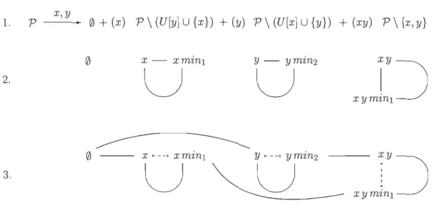
Lemma 1. If a poset P has only two minimal elements, then there is a Hamiltonian cycle of down-sets in P in which two down-sets differ by one or two elements and such that
0
is adjacent to each of these two minimal elements.Proof. Let P be a poset that has only two minimal elements x and y. By applying the generalized recurrence of Proposition 1, Equation (1.2), we obtain the first line of Figure 1.10. On the right side of the arrow we have 4 parts, the first of whicb is
0.
The first part is empty since the poset has only two minimal elements. Let minl be a minimal element of the second part. In this case, it is also a minimal element of the fourth part since Y \ (U
[y]
U{x})
ç
Y \{x,
y}.
Let min2 be a minimal element of the third part. According to Theorem l, there is a Hamiltonian cycle of the down-sets of the second part containing the edge{lb,
mind. Since x is included in every down-set of this cycle, this cycle contains the edge {x, x mind. By an argument similar to the previous one, there are two cycles of down-sets for the third and fourth parts containing, respectively, the edges {y, y min2} and {xy, x y mind. These cycles are on the secondx,Y
1. p
- - - . 0
+
(x) p \ (U[y]u
{x})+
(y) p \ (U[x]u
{y})+
(xy) p \ {x,y}x - xmznl y - y min2
2.
U
U
X >---, xminl y>---,y min2
3.
U
U
Figure 1.10. Illustration of Lemma 1.
line of Figure 1.10. On the third li ne we removed sorne edges and added others to ob tain the required Hamiltonian cycle. The dashed lines are the removed edges. We can easily verify that when one or more among the second, third and/or fourth parts are empty the corresponding cycles are reduced to one element and we always have a Hamiltonian cycle of down-sets in which two adjacent down-sets differ by one or two elements, with
0
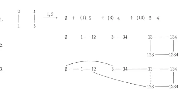
being adjacent to each of these two minimal elements. 0Example 5. Consider the poset on the left side of the first line of Figure 1.11. By
choosing 1 and 3 for the minimal elements (the elements x and y) and applying Lemma
1, we obtain the first line of Figure 1.11. The first part is the empty poset whose un derlying set is
0;
consequently it has the Hamiltonian cycle0.
The second part is the empty poset whose underlying set is 2; therefore it has the Hamiltonian cycle{0,
2}.By adding the element 1 to each ideal of this last cycle we obtain the Hamiltonian cycle
{1,12}. The third part is the empty poset whose underlying set is 4; therefore it has the
Hamiltonian cycle {0,4}. By adding the element 3 to each ideal of this last cycle we obtain the Hamiltonian cycle {3,34}. The fourth part is the empty poset whose under
1. 2 1 4 1 1,3 0
+
(1) 2+
(3) 4+
(13) 2 4 1 3 0 1-12 3-34 13 134 2. 1 1 123 1234---
3. 0 - 1 - 1 2 3-34 13 134 1 123 1234Figure 1.11. Example illustrating the use of Lemma 1.
lying set is {2, 4},. therefore it has the Hamiltonian cycle {0, 2, 24, 4}. By adding the set
13 to each ideal of this last cycle we obtain the Hamiltonian cycle {13, 123, 1234, 134}.
The Hamiltonian cycle of each part is on the second line of Figure 1.11.
Since we applied Lemma 1, we add the edges {0, 1}, {0,3}, {12,123} and {13, 34}, and remove the edge {13,123}, but according to Remark l, we do not remove the edges
{1,12} and {3,34}. Thus, we obtain the required Hamiltonian cycle on the third line of Figure 1.11, where
0
is adjacent ta each of the ideals 1 and 3.Lemma 2. If a poset P has at least two minimal elements, then there is a Hamiltonian cycle of down-sets in P in which two dawn-sets differ by one or two elements and such that
0
is adjacent ta each of these minimal elements. In addition, if two of these minimal elements are overlined, then each of the new posets obtained has only one overlined minimal element (it may have other minimal elements that are not overlined).Proof. (By induction on n, the number of minimal elements in P).
----
---x,y
l.P---'-· P\U[x,y]
+
(x) P\(U[Y]U{x})
+
(y) P\(U[x]U{y})
+
(xy) P\{x,y}
y - - yz
o
U
2. 1 z 3.o
-
x .---. xz
y .---. yz
xy
l~---===---U
U_ _
J)
4.z - 0-tz
y - - yz
~
U
5.z·----·
0 .--.
tz
x .---. xz
y .---. yz
U
~ ~
.. ~ " . ~---_.__...__
._...._.... 6.t - 0 - z
x - - xz
y - - yz
~
U
U
7.t·----·
0 .--.
z
x .---. xz
y .---. yz
U
~ ~
---_._._
__ .Figure 1.12. Illustration of Lemma 2. Lines 2-3 cover Case 1, lines 4-5 cover Case 2 and lines 6-7 cover Case 3.
(Equation 1.2), with initial values D =
0
and Y = E and the minimal elements x andy, we obtain the first line in Figure 1.12. We note that the first part is included in each of the second, third and fourth parts.
Consequently, if the first part has a minimal element, it will be also a minimal element of each of the other three parts.
Basic step. If n = 2, then the result follows from the proof of Lemma 1. Moreover, as we require minI to be adjacent to
0
for the second and fourth parts and that min2 be adjacent to0
for the third part (see Figure 1.10), each of these three parts will have an overlined minimal element according to Remark 2.Induction step. If n
>
2, then we have 3 cases.1. The first part restricted to
Y\U[x,
y]
contains a unique elementz.
Then there is a Hamiltonian cycle for this part that contains the edge{0,
z}.
Sincez
is a minimal element in each of the second, third and fourth parts, according to Theorem 1 these parts have the cycles indicated in li ne 2 of Figure 1.12. We note that one or more of the last three cycles may be reduced to one edge if the number of elements of the corresponding poset is restricted to one element. Consequently, the required Hamiltonian cycle of P is shown in the third line of Figure 1.12.2. The first part restricted to Y \
U[x,
y]
contains more than one element but exactly one minimal element z. This minimal element certainly has a covert.
Applying Theorem l, Case 2, we obtain the first Hamiltonian cycle on the fourth line in Figure 1.12. The other Hamiltonian cycles on the same line are also obtained by applying Theorem 1 with z as median element. Consequently, the cycle of P is shown on the fifth line of the same figure.3. The first part restricted to Y \
U[x,
y]
has at least two minimal elements, say t andz. By the induction hypothesis there is a Hamiltonian cycle with
0
adjacent to tand
z
as shown on the sixth line. The other Hamiltonian cycles on the same line are obtained as in Case 2 except that the median for the fourth part is t insteadof z. Finally, the cycle of P is shown on the seventh line of the same figure. Analogously to the basic step, we can show that each of the second, third, fourth and possibly the first will have an overlined minimal. 0
Figure 1.12 does not include overlines because it shows a general poset, and the overlines are a function of the Hasse diagram of a particular poset.
A situation is called blocked ""hen we require
°
to be adjacent ta two elements, i.e. when we have 2 minimal elements, each of which is overlined. In such a situation, we use Lemma 2 to unblock this situation. Then we obtain new posets, each of which has one overlined minimal element. It follows that each time we use Lemma 2 (our generalization of Squire's recurrence) we return to the choice of median 3 or 4 times (depending upon the first part) where we apply Theorem l, 2 or 3 as needed to the new posets.Example 6. Consider the poset on the left side of the first line of Figure 1.13. By choosing 2 and 4 for the minimal elements x and y and applying Lemma 2, we obtain the first line of Figure 1.13. The first part is the empty poset whose underlying set is
{1}; consequently it has the Hamiltonian cycle {0,1}. The second part is the empty
poset whose underlying set is {l, 3}; therefore it has the Hamiltonian cycle {0, l, 13, 3}. By adding the element 2 to each ideal of this last cycle we obtain the Hamiltonian cycle {2, 12, 123, 23}. The third part is the empty poset whose underlying set is
{l, 5};
therefore it has the Hamiltonian cycle
{0,
l, 15, 5}. By adding the element 4 to each idealofthis last cycle we obtain the Hamiltonian cycle {4, 14, 145,45}. Thefourth part is the empty poset whose underlying set is {l, 3, 4}; therefore by applying Theorem 1 and by taking 1 for the minimal element we can show that this poset possesses a Hamiltonian cycle having the edge
{0,
1}. By adding the set 24 to each ideal of this last cycle we obtain a Hamiltonian cycle having the edge {24, 124}. The Hamiltonian cycle of each part is on the second line of Figure 1.13.--'--... 1 + 2 1 3
+
(4)l
5+
(24)l
3 5 1. 1 1 1"2
"4
o
2 - 1 2 4 - 141
2 4 ) 2. 1 1 1 1 1 1 13-123 45-145 3.0JdJI·----·
Y
ï----·
Y-
Y
J
: 13-123 45-145 : 1:::= _ _ 124Figure 1.13. Example illustrating the use of Lemma 2.
and remove the edges {2,12}, {4,14} and {24, 124}. We finally remove, according to Remark 1) the edge
{0,
1}. Thus we obtain the required Hamiltonian cycle on the thirdline of Figure 1.13) where
0
is adjacent to each of the ideals 2 and 4.1.
7
Hamiltonian
cyclewhen there are at least two elements less than
the median
The following Lemma 3 is a necessary step for the proof of Theorem 3.
Lemma 3. Let P be the pos et P
=
Q+
R (disjoint union of two posets). Let {x 1, X2,... ,Xn } be the underlying set of Q) where n ~ 2, and X n be maximal. Then there is a Hamiltonian cycle of down-sets in P in which two adjacent down-sets differ by one or two elements and this cycle contains the edge {X1X2 ... Xn-l, X1X2 ... xn }.
Pro of. (By induction on n) .
Basic step. If n
=
2, then we have 2 cases.Xm = Xl 1. P P\
{xd
+
(Xl) P\{xd
0
Xl 2. via via first second part part X2 Xl X2 via via 3. first second part part X2 - - Xl X2 ---.--'Figure 1.14. First case of the basic step in Lemma 3.
(1.1) with Xl as median we obtain the first line of Figure 1.14. In this case,
P\{xd
has a minimal element X2. According to Theorem 1, the cycles of the first and second parts contain the edges
{0,
xû
and {Xl, XIX2}, respectively, that are onthe second line of Figure 1.14. Also according to Theorem 1, Case 1, applied to P with Xl as median, we add the edges {Xl,
0}
and {XIX2, X2} and remove theedges
{0,
xd
and {Xl, XIX2}. Then we obtain the required Hamiltonian cycleon the third line of the same figure. We note that this cycle contains the edge
{Xl, XIX2}.
2. If Xl
<
X2, then by applying equation (1.1) with Xl as median we obtain the firstline of Figure 1.15. We distinguish 2 cases.
(a) IfP\U[XI] =
0,
then P\{xd
= {X2}' In this case the cycle of the first part is0
and the cycle of the second part contains the edge {Xl,xIxd.
Accordingto Theorem 1, Case 2, applied to P with Xl as median, we add the edges
{0, xd
and{0,
XIX2} and, according to Remark 1, we do not remove the edge{Xl, XIX2}. Then we obtain the required Hamiltonian cycle on the second
line of Figure 1.15. We note that this cycle contains the edge {Xl, XIX2}.
Xm = Xl 1.
P
P \{xI}
2. Xl X2o
XI- Xl X2 - - - - . . 3. via via first second part part - - - min - -Xl min - - - "Figure 1.15. Second case of the basic step in Lemma 3.
them and caU it min. According to Theorem 1 with min as median, there is a Hamiltonian cycle containing the edge
{0,
min}. On the other hand, the second part has at least two minimal elements: min and X2. By applying Theorem 1, Case 1, with X2 as median, we obtain a. Hamiltonian cycle in which0
is adjacent to min and to X2. By adding Xl to each down-set ofthis cycle we obtain a Hamiltonian cycle in which Xl is adjacent to xlmin
and XIX2. Since we applied Theorem 1, Case 1, to P with Xl as median, we
add the edges
{0,
Xl} and {min, Xl min} and remove the edges{0,
min} and{Xl, Xl min}. FinaUy, the required Hamiltonian cycle of P is on the third !ine of Figure 1.15. We note that this cycle contains the edge {Xl> Xl X2}'
Induction step. If n
>
2, then without loss of generalicy, Xn will not be chosen as median. In addition, we suppose that the median Xm is chosen among the elementsXIX2 ... Xn-l. We distinguish three cases.
1. #(D[xm ]) = 2, i.e. Xm covers a unique element, say Xm-l' Then this last element
is minimal. By applying Theorem 2 with X m as median we obtain the first line
cording to Theorem 1, there is a Hamiltonian cycle containing the edge
{0,
xm-d.For the second part there are three cases.
(a) If n
=
3 and E contains only 3 elements, then the cycle of the first part is the edge{0,
xd
and the second part is the singleton {X3}' Consequently X3is a minimal element in the second part. By applying Theorem 1 with X3
as median we obtain the Hamiltonian cycle {XIX2, XIX2X3} since D[xm ] =
XIX2. Since we applied Theorem 2 to P, we add the edges
{0,
XIX2} and {Xl, Xl X2X3} according to Remark 1, we do not remove the edge {0,xd
northe edge {XIX2, XIX2X3}. Finally we obtain the required Hamiltonian cycle containing the edge {XIX2, XIX2X3} on the second line of Figure 1.16.
(b) If n
=
.3 and E contains more than three elements, then the cycle of the first part contains the edge{0,
xd
and the second part has at least two minimal elements: X3 and another one, say min. By applying Lemma 2we obtain a Hamiltonian cycle containing the edges {XIX2, XIX2X3} and {XIX2, xlx2min}. Since we applied Theorem 2 to P, we add the edges
{0,
XIX2} and {Xl, xlx2min} and remove the edges{0,
xd
and {XIX2' xlx2min}. Finally we obtain the required Hamiltonian cycle containing theedge {XIX2, XIX2X3} on the third line of Figure 1.16.
(c) If n
>
3, then the second part contains at least two elements from the set{Xl, X2,"', x n } and by the induction hypothesis there is a Hamiltonian cycle
of down-sets containing the edge {XIX2'" Xm-2Xm+1 ... Xn-l, XIX2'" Xm-2Xm+1 ... x n }. When we add to each down-set of the last cycle the set D[xm ]
=
Xm-IX m , this cycle will contain the edge { XIX2'" Xn-l, XIX2 ... x n }.In addition, when we apply Theorem 1 to the second part with the median, which we call min, this last cycle will contain the edge {Xm-IX m , xm-Ixmmin}.
Since we applied Theorem 2 to P, we add the edges
{0,
Xm-IX m } and {Xm-l' xm-Ixmmin} and remove theedges{0,
xm-d and {Xm-IX m , Xm-IX m min}. Finally we obtain the required Hamiltonian cycle containing the edge2. If#(D[xml)
=
1, then when we apply Theorem 1 with X m as median, the first partwill either have a Hamiltonian cycle of down-sets containing the edge
{0,
min},where min is a minimal element of the poset of the first part, or will have the
cycle
0,
depending upon whether the first part is non-empty or empty. As for the second part, its underlYlng set contains at least two elements from the set{Xl, X2, " ' , x n }· By the induction hypothesis, and by an argument similar to
the one applied to the second part in Case 1 (c), there is a Hamil tonian cycle of down-sets containing the edge {Xl X2 ... Xn-l, Xl X2 ... x n }. Moreover, when we apply Theorem 1 to this second part with min as median, this last cycle will
contain the edge {xm,xmmin}. Finally, by applying Theorem 1 to P, Case lor 2, with Xm as median, depending upon whether the first part is non-empty or empty, and adding and removing the appropriate edges we obtain the required Hamiltonian cycle containing the edge { XIX2'" Xn-l, XIX2'" x n }.
3. In this case #(D[xml)
>
2. By applying equation (1.1) to P with Xm as median, we obtain the first line of Figure 1.16. We suppose that Xm does not have any brothers (if Xm has a bl'Other we choose as median another elements that has no brothers) and that D[xm ] \ {xm} = {Xi, " ' , xm-d, which must have a maximal element in P, say Xr . Since #(D[xml)
>
2, the first part contains the set {Xi, .. " xm-d, whlch contains at least two elements. By the induction hypothesis there is a Hamiltonian cycle of down-sets containing the edge
{Xi'" Xr-l Xr+l'" Xm-l, Xi' ,. xm-d· By an argument similar to that of Case 1 above with all its subcases, there is a Hamiltonian cycle of down-sets for the second part containing both edges {XIX2'" Xn-l, XIX2'" x n } and {Xi'" X m , Xi'" xm min}.
Finally by adding the edges {Xi' .. Xr-l Xr+l ... Xm-l,
Xi ... x m } and {Xi' .. Xm-l) Xi' .. X m min} and removing the edges {Xi' .. Xr-l Xr + l
... Xm-l, Xi'" xm-d and {Xi'" Xm, Xi'" x m min} we obtain the required Hamil
tonian cycle containing the edge { XIX2' .. Xn-l, XIX2 ... x n } on the fifth line of Figure 1.16. We note that if Xn-l is greater than each element of {Xl,' " , Xn -2}
-Xm
P \
U[Xm]+
(D[x m])P \
D[xm] 1.P
2. via first part (/) Xl x2 1 X l - - Xl X2 X3 via second part 3. vIa first part (/) Xl X2 - Xl X2 X3 via second Xl - - Xl x2 min part (/) Xm-IX m --XI"'Xn-1 ;, , , ,, , via via second part 4. first part xm-Ixmmin ... - - XI"'Xn Xm-l Xi ... Xm-l \ Xr - - Xi' .. Xm - - Xl" 'Xn-l 5. via via ,, , , firstpart second part .
Xi'" Xm-l Xi'" xmmin - - - XI"'X n
Figure 1.16. The induction step of Lemma 3.
other cycle containing the edge {Xl'" Xn-2, Xl ... xn-d, Consequently, we avoid
this choice in that case. 0
Remark 3. In Lemma 3, we proved that there is a Hamiltonian cycle of down-sets of the poset satisfying Lemma 3 's hypothesis, where two adjacent down-sets differ by one or
two elements and this cycle contains the edge {XIX2'" Xn-l, XIX2'" xn }. When apply ing Squire 's recurrence (Equation (l.I)) to this poset with the median Xm chosen among
{Xl, X2, ... Xn } we noticed that the set D[xm] is added to each element of the cycle of the
second part (see the first line of Figure 1.16), and induction on this second part enabled us to prove the existence of the edge {XIX2'" Xn-l, XIX2'" x n }. On the other hand, if
we chose the median Xm outside the set {Xl, X2, ... xn}, the set D[xm ] would be added
to each element of the cycle of the second part, but we do not want D[xm ] to be added
to the elements of our cycle which will contain the edge {X1X2"'Xn-l, X1X2···Xn}. Consequently, in this case this last edge is part of the cycle of the first part.
Remark 4. The choice of Xn as median is the last among the elements of the set {Xl, X2, "', Xn}. This last choice ensures the existence of the edge
{0,
Xn} to which we must add the set X1X2 ... Xn-l built at this stage and this ensures the existence of the edge {X1X2 ... Xn-l, X1X2" . Xn} by creating it. In practice, we underline each element of the set X1X2 ... Xn (we draw a line under it) and these underlines will be transferred to the first part when Xm is chosen outside the set {Xl, X2, ... , xn} and to the secondpart when it is chosen among the elements of this set so that Xn will be chosen after the elements {Xl, X2, "', xn-d·
Remark 5. Given the existence of the edge {XIX2' .. Xn-l, XIX2 ... xn} in Lemma 3, the edge
{0,
Xn} must exist in a sub-cycle. Therefore, Xn, which is underlined, is also considered overlined. Consequently, this Xn cannot be chosen as median unless it is the unique element in the poset, since at this stage it loses its connection with0
and regains it when we add the edge {0, Xn}.Two elements are said to be brothers if there is a third one which is covered by each of them.
Theorem 3. Let E be the underlying set of elements of the poset P of which X is an element having at least 2 elements less than it and do es not have any brothers. There is a Hamiltonian cycle of down-sets of this poset where two adjacent down-sets differ by one or two elements and this cycle does not contain the edge {XIX2' .. Xk-l, XIX2" . xd, where XIX2 ... XkX = D[x] and Xk is maximal in P \ U[x].
1 1. X2 X m = X 1 Xl 2. 3.
Figure 1.17. First subcase of first case in Theorem 3.
Xm
=
X 1. - - - . . Xl ( / ) - - Xl 2. 1 1 X2 - - XIX2 3.Figure 1.18. Second subcase of first case in Theorem 3.
1. In this case n
=
3 and there are two elements less than x. We have 2 sub-cases, where the poset is the left side of the first line of either Figure 1.17 or Figure 1.18. By applying Equation (1.1) with X as median we obtain the first line ofeither Figure 1.17 or Figure 1.18. The Hamiltonian cycles of down-sets of first and second parts are on the second line of the same figure. By adding the edges
{x Xl X2,
xd
and{x XIX2, Xl X2}
and removing the edge {Xl, Xl X2} we obtainthe required Hamiltonian cycle on the third line which does not contain the edge
{Xl, XIXÛ'