HAL Id: hal-01101144
https://hal.inria.fr/hal-01101144
Submitted on 9 Jan 2015
HAL is a multi-disciplinary open access
archive for the deposit and dissemination of
sci-entific research documents, whether they are
pub-lished or not. The documents may come from
teaching and research institutions in France or
L’archive ouverte pluridisciplinaire HAL, est
destinée au dépôt et à la diffusion de documents
scientifiques de niveau recherche, publiés ou non,
émanant des établissements d’enseignement et de
recherche français ou étrangers, des laboratoires
Hermes: a simple and efficient algorithm for building
the AOC-poset of a binary relation
Anne Berry, Alain Gutierrez, Marianne Huchard, Amedeo Napoli, Alain
Sigayret
To cite this version:
Anne Berry, Alain Gutierrez, Marianne Huchard, Amedeo Napoli, Alain Sigayret. Hermes: a simple
and efficient algorithm for building the AOC-poset of a binary relation. Annals of Mathematics and
Artificial Intelligence, Springer Verlag, 2014, 72 (1), pp.45-71. �10.1007/s10472-014-9418-6�.
�hal-01101144�
AMAI manuscript No.
(will be inserted by the editor)
Hermes: a simple and efficient algorithm for building the
AOC-poset of a binary relation
Anne Berry · Alain Gutierrez · Marianne Huchard · Amedeo Napoli · Alain Sigayret
Friday 7thMarch, 2014, 16:03 / Received: Second revision / Accepted: date
Abstract Given a relation R ⊆ O × A on a set O of objects and a set A of attributes, the AOC-poset (Attribute/Object Concept poset), is the partial order defined on the “introducers” of objects and attributes in the corresponding concept lattice. In this paper, we present Hermes, a simple and efficient algorithm for
building an AOC-poset which runs inO(min{nm, nα}), wherenis the number of objects plus the number of attributes,mis the size of the relation, and nαis the time required to perform matrix multiplication (currentlyα= 2.376). Finally, we compare the runtime of Hermeswith the runtime of other algorithms computing
the AOC-poset:Ares,CeresandPluton. We characterize the cases where each
algorithm is the more relevant.
1 Introduction
A concept lattice –also called a Galois lattice [3]– provides a powerful support for data analysis and knowledge discovery. Such a lattice is built w.r.t. a binary relation between a set of objects and a set of attributes. However, the concept lattice may have an exponential size in the number of objects or attributes. A canonical sub-order of the lattice is the so-calledAOC-poset for Attribute/Object Concept poset (the term was coined in [29, 27]), which is of much smaller size. Thus, it can be recommended in some specific applications, as it contains all the relevant information for retrieving all formal concepts. In the general case, it can be used to save space and simplify visualization. The AOC-poset is based on the key elements of the lattice: object-concepts and attribute-concepts [16], also called introducers
Anne Berry, Alain Sigayret
LIMOS (CNRS UMR 6158 - Universit´e Clermont-Ferrand II), Clermont-Ferrand (France)? E-mail: berry, [email protected]
Alain Gutierrez, Marianne Huchard
LIRMM (CNRS UMR 5506 – Universit´e de Montpellier II), Montpellier (France) E-mail: alain.gutierrez, [email protected]
Amedeo Napoli
LORIA (CNRS UMR 7503 – Inria Nancy Grand Est – Universit´e de Lorraine), Vandoeuvre-l`es-Nancy (France) E-mail: [email protected]
in the rest of this paper. The number of introducers is at most equal to the number of objects plus the number of attributes (denoted by n hereafter). Furthermore, the AOC-poset includes all the join-irreducible and the meet-irreducible elements of the concept lattice.
Depending on the background of the authors, several names were given for de-noting the same structures, asGalois lattice andconcept lattice,Galois sub-hierarchy
andAOC-poset. Some other names were also used such as knowledge space in [25] for knowledge representation purposes, pruned concept hierarchy in [18] for class inheritance hierarchy restructuring, Galois sub-hierarchyin [11] again for class in-heritance hierarchy restructuring and property sharing, and finallyAOC-poset in [26, 29, 27] for building classifications from linguistic data and in [19] for applica-tions of Formal Concept Analysis (FCA) to non-monotonic reasoning.
In this work, we decided to use the expressionAOC-posetas it gives a direct idea and image of the structure that is actually built by the algorithm discussed in this paper. Three algorithms for building AOC-posets already exist, namelyAres[10], Ceres [22], and Pluton [5]. Each of them has a time complexity of O(n3) and is somewhat complex to implement. A comparison of their experimental running times was investigated in [2]. Following and completing this line of work, we present in this paper a new algorithm for building the AOC-poset of a binary relation, calledHermes, which has a better complexity.Hermesruns inO(nm) time, where
mis the size of the relation, and is easy to understand and to implement. With more effort invested in the implementation,Hermes can be made to run inO(nα) (i.e. O(n2.376)) time, which is the time for performing matrix multiplication.Hermes
works by simplifying and then extending the input relation into a relation which contains in a compact form all the necessary information on the elements of the AOC-poset.
In this paper, we also conduct a comparative analysis of the running time of the four algorithms on randomly generated binary relations as well as on some real case studies. Lessons are learned from this analysis, and we propose, for each algorithm, a characterization of the cases where it is more efficient that the others. The paper is organized as follows: after this introduction, we give some no-tations and definitions. Section 3 motivates the use of AOC-posets by some rep-resentative applications. Section 4 proves some preliminary results and presents the algorithmic tools necessary to ensure our good complexity. Section 5 describes and analyzes in detail the successive steps of our algorithmic process. Section 6 briefly outlines how previous algorithms work and compares their complexity with that of Hermes. Section 7 describes the special case for chordal bipartite
rela-tions, where the final relation can easily be obtained inO(n2) time. In Section 8, we compare the runtimes of the existing algorithms that compute the AOC-poset and we provide the most relevant application cases for each algorithm. We con-clude in Section 9. An appendix gives more details about the runtimes through representative graphics.
2 Definitions and notations
In this section, we specify the notations that are used in the paper. Given a finite set O of objects and a finite set A of attributes, a binary relation R ⊆ O × A
thestarting set of the relation. The cardinal of a setX is denoted by|X|and then
n=|O|+|A|andm=|R|. The relation between objects and attributes through
Ris written as follows:
– For (x, y)∈ R, we say thatxis anantecedent ofyand thatyis animage ofx.
– For x ∈ O,R(x) ={y ∈ A |(x, y)∈ R}is theimage set (row) of x,
– For y ∈ A,R−1(y) ={x ∈ O |(x, y)∈ R}is theantecedent set(column) ofy.
– For X ⊆ O,R(X) ={y ∈ A | ∀x ∈ X,(x, y)∈ R}is the image set ofX,
– For Y ⊆ A,R−1(Y) ={x ∈ O | ∀y ∈ Y,(x, y)∈ R}is the antecedent set ofY. Regarding notations, it can be noticed that in [16] the notationx0 is used for
R(x) and y0 for R−1(y), and that the triple (O, A, R) is called a formal context
(see the comparison below). Actually, the relationRcan be considered from four points of view as discussed in [37, 13, 14], and the way how Ris considered here and in FCA is one of these four points of view.
A maximal rectangleX × Y ofRis such that∀x ∈ X, ∀y ∈ Y, (x, y)∈ Rand
∀w ∈ O − X, ∃y ∈ Y | (w, y)6∈ R and ∀z ∈ A − Y,∃x ∈ X | (x, z)6∈ R. Such a maximal rectangleX × Y is also called aformal concept and denoted by (X, Y) in [16], whereX is called theextent andY theintent of the concept (X, Y). In the following, the extent and the intent of a conceptC are also denoted byExtent(C)
andIntent(C). The concepts, ordered by inclusion w.r.t. their extents –or dually w.r.t. their intents– form a complete latticeL(R) called aconcept latticeor aGalois lattice. For two conceptsCandC0,C <L(R)C0means thatExtent(C)⊂ Extent(C0)
(dually Intent(C0) ⊂ Intent(C)). A concept lattice is represented by its Hasse diagram, where reflexivity and transitivity edges are omitted.
Theobject-concept of the objectxis a concept denoted byCxwhichintroduces x, i.e. x is in the extent of Cx but is not in the extent of any smaller concept C <L(R) Cx. Dually, theattribute-concept of the attribute y is a concept denoted
by Cy which introduces y, i.e. y is in the intent of Cy but is not in the intent
of any greater concept C >L(R) Cy. Actually, the intent of the object-concept Cx corresponds to R(x) and the extent of the attribute-concept Cy corresponds
to R−1(y). The expressions object-concept and attribute-concept were introduced in [16], where the object-concept is denoted by γx= (x00, x0) and the attribute-concept by µy = (y0, y00). Based on the correspondences x0 = R(x) and y0 =
R−1(y), it comes thatγx= (R−1(R(x)), R(x)) whileµy= (R−1(y), R(R−1(y))).
Object-concepts and attribute-concepts are called in the present paper intro-ducer concepts or simplyintroducers. Objects are introduced from bottom to top and attributes from top to bottom in L(R), meaning that once an attribute is introduced, it is inherited by all concepts which are below. Dually, once an ob-ject is introduced, it is “inherited” by all concepts which are above: actually this is also related to reduced notation of concept lattices. A given concept may in-troduce several objects and/or attributes. In addition, it can be noticed that in [16] the so-calledarrow relations are used to characterize the relationship between attribute-concepts and object-concepts, but without referring to AOC-posets.
A relation is said to be clarified when it has no identical lines (row or col-umn, and hereafter, the term line is indifferently used for row and column). A relation is said to be reduced when it is clarified and has no row which is the intersection of several other rows, and no column which is the intersection of sev-eral other columns (“clarification” and “reduction” are taken from [16]). When a relation is reduced, the introducers exactly correspond to meet-irreducible and
join-irreducible elements, to which we should add the top if it introduces an at-tribute, and the bottom if it introduces an object. In a non-reduced relation there are extra introducers. Recall that a meet-irreducible (resp. join-irreducible) ele-ment x in a lattice is not the meet (resp. join) of any subset of elements not containingx.
Running example. Figure 1 shows the concept latticeL(R) (as drawn by Concept Explorer [38]) and the AOC-poset AOC(R) of relation R. In L(R), concept (1, acdeg) intro-duces 1 (reduced label: 1), concept (1346, c) introduces c (reduced label: c), and concept (3, abcdf g) introduces 3 and b (reduced label: 3, b). All these concepts are in AOC(R); con-cept (13, acdg) introduces nothing (reduced la-bel empty) and as such is not in AOC(R).
R a b c d e f g 1 × × × × × 2 × × × × 3 × × × × × × 4 × × 5 × 6 × × 7 × × × 8 × × × × L(R) AOC(R)
Fig. 1: LatticeL(R) and AOC-posetAOC(R), both with the reduced labeling, for our running example.
AOC(R) denotes theAOC-posetof relationR, defined by the set of introducers concepts ordered as inL(R), i.e.AOC(R) is a sub-order ofL(R). The elements of
AOC(R) are labeled by the objects and/or attributes that they introduce and they define thereduced labeling, that can be applied toL(R) [16]. In reduced labeling, some concepts may possibly have an empty label. The symbol<AOC(R) denotes the partial ordering used to compare two elements ofAOC(R), as <L(R) is used forL(R). Finally, alinear extension of a partially ordered setP is a total order in whichP is included.
Below, we present the correspondences between FCA notations and theHermes
FCA notations Hermesnotations context (G, M, I) context (O, A, R) x ∈ Gandx0 x ∈ OandR(x) X ⊆ GandX0 X ⊆ OandR(X) y ∈ M andy0 y ∈ AandR−1(y) Y ⊆ M andY0 Y ⊆ AandR−1(Y) object-conceptγx= (x00, x0) γx= (R−1(R(x)), R(x)) attribute-conceptµy= (y0, y00) µy= (R−1(y), R(R−1(y)))
x ∈ Gandx00 DomO(x) y ∈ Mandy00 DomA(y)
3 State of the art and motivation for studying the AOC-poset
In this section, we discuss preceding work on the AOC-poset and related applica-tions that motivated its definition and use.
Mineau et al. [25] introduced the term of knowledge space in the context of conceptual clustering of conceptual graphs, to designate the AOC-poset built w.r.t. a relation associating objects and triples representing edges of the conceptual graph and generalizations of these edges (with a joker symbol). To the best of our knowledge, this is the first paper using this structure, and this is done in a specific case where each object owns a specific attribute (not owned by the other objects). The notion of “knowledge space” was then reused in [17] in an object-oriented software engineering context. The knowledge space is called in [18] apruned con-cept hierarchyor apruned concept inheritance hierarchywhen the labels are reduced. In these papers, a class inheritance hierarchy is flattened into a table that asso-ciates the classes with their members (class properties and methods). The pruned concept hierarchy is used to understand the structure of the sub-typing relations and to restructure the class inheritance hierarchy, so that it is better factorized, eliminating redundancies. The termGalois sub-hierarchy was introduced in [9, 10] when the Ares algorithm was defined. Galois sub-hierarchies were also used in
object-oriented software engineering for restructuring class inheritance hierarchies [11]. A state of the art paper [21] shows that several approaches used in software engineering actually build the AOC-poset or characteristic parts of it, often with-out mentioning at all concept lattices, revealing that the AOC-poset appears as a natural partial ordering for the targeted applications. This can be explained by the fact that a class inheritance hierarchy corresponds to a conceptual structure where useful attributes such as variables and methods are introduced. In our ex-perience, proposing new classes to a designer in order to remove redundancy is appreciated and often reveals hidden abstractions, whereas proposing new classes that only merge some inherited properties and methods is rarely useful.
The termAOC-poset was introduced in [29, 27]. AOC-posets were also used in applications of FCA to non-monotonic reasoning and domain theory [19], and to produce classifications from linguistic data [26, 29, 27], because of their capability to structure knowledge. Specific parts of the AOC-poset –mainly attribute-concepts– were used in several works, including refactoring of a class hierarchy (e.g. [18] as already mentioned), and more recently for extracting a feature tree from a set of products variants in Software Product Lines [31]. It appears that Formal Concept Analysis and AOC-posets are very useful in this research domain [23, 36, 35] as the
problem is to find in a set of software variant commonalities, differences, as well as exclusion and implication constraints that can be extracted from the associated concept lattice.
In a recent work [12], authors use AOC-posets –and the Hermes algorithm–
instead of concept lattices in the context of Relational Concept Analysis [30], for extracting all the implication rules having a single element in the left hand side within a large database on river streams. A low computation time is needed for providing quick answers to domain experts during working sessions and for rapidly analyzing several datasets coming from the whole database.
AOC-posets also help classifying components in subtyping-based directories [1]. Classification and retrieval operations in directories based on AOC-posets versus directories based on concept lattices are compared. Results show the efficiency and availability of the AOC-poset in real case studies, while concept lattices often are too complex and too large to be wholly computed and traversed, especially in dynamic environments when components are added and removed on-the-fly.
In the case of knowledge representation and class inheritance hierarchy ap-plications, the concepts and the covering relation are needed because they are transformed as syntactical primitives including classes/objects, attributes, method declarations (concepts), or inheritance declarations (class covering relation). In software product line applications, the concepts coming from the formal context mapping products to features are used for building variation points, while the covering relation captures relations between the variation points.
Three algorithms have been proposed [2, 22, 10], whose principles and com-plexity are discussed in Sect. 6. In [2], an experimental comparison of these three algorithms was provided, which is discussed and compared with the current work in Section 8.
4 The structure of the AOC-poset
We now present the basis of Hermes, our new algorithm for computing an
AOC-poset, which works in a simple way. It computes the inclusion order in the set of attributes and concatenates this information with the input relation, providing the whole information required to extract the corresponding AOC-poset.
4.1 The domination relation on attributes and objects
First, we need to compare the introducers and to order them. We rely on the follow-ing propositions, which transpose to AOC-posets well-known results for concept lattices presented in [16].
Proposition 1
Let Cxbe the introducer of x ∈ O and Cy be the introducer of y ∈ A. Then:
– Cx≤AOC(R)Cy iff(x, y)∈ R. – If Cx>AOC(R)Cy then(x, y)6∈ R.
In the first case, Cx≤AOC(R)Cy means that the intent ofCx (corresponding
to R(x)) contains the intent ofCy which itself includesy, and thusy ∈ R(x) or
(x, y)∈ R. In the second case,Cx>AOC(R)Cymeans thatxis not in the extent of
any smaller concept, and thus not in the extent ofCy, i.e.x 6∈ R−1(y) or (x, y)6∈ R.
In [32], the notion of domination is introduced, which originates from graph theory: domination in a relation stemmed from the notion of domination in the co-bipartite graph which is the complement of the bipartite graph induced by the relation.
An attribute y ∈ A is said to dominate an attribute z ∈ A in R if the an-tecedent set ofyis included in the antecedent set ofz, i.e.R−1(y)⊆ R−1(z); the corresponding relation is denotedDomA. When the inclusion is strict, the
dom-ination is said to be strict. For y ∈ A, DomA(y) = {z ∈ A | R−1(y) ⊆ R−1(z)}
is the set of all attributes dominated by y. Actually, DomA defines the way
how attributes are labeling the concepts ofAOC(R) from the bottom –the domi-nating attributes– to the top –the dominated attributes. In the running example,
R−1(b) = {3} ⊂ R−1(a) = {1,2,3,7,8}, i.e. attribute b dominates attribute a
and the introducer ofbis smaller than the introducer of a, as shown in Figure 1.
DomA(b) ={a, b, c, d, f, g}. Recall that in FCA notations,y0corresponds toR−1(y)
and thusDomA(y) corresponds toy00.
A domination relation,DomO, can also be defined between objects by inclusion
of their image sets:∀x ∈ O, DomO(x) ={w ∈ O | R(x)⊆ R(w)} is the set of all
objects dominated byx. The label ofAOC(R) will be set from top (the dominating objects) to bottom (the dominated objects), according to the dual behavior of objects and attributes in concepts. In our running example,R(6) ={c, d} ⊂ R(1) =
{a, c, d, e, g}; object 6 dominates object 1 and the introducer of 6 is greater than the introducer of 1.DomO(6) ={1,3,6}. Again, Recall that in FCA notations,x0
corresponds toR(x) and thusDomO(x) corresponds tox00.
We can summarize the above discussion by the following proposition (see also [6]):
Proposition 2
– Endowed with the domination relation DomA, the set of attribute-concepts of R forms a sub-order of AOC(R): for y, z ∈ A, the introducer of y is smaller than or equal to the introducer of z iff y dominates z (or z ∈ DomA(y)).
– Endowed with the domination relation DomO, the set of object-concepts of R forms a sub-order of AOC(R): for x, w ∈ O, the introducer of x is greater than or equal to the introducer of w iff x dominates w (or w ∈ DomO(x)).
4.2 Computing the domination relation
We will need two operations for establishing the complexity results related to our algorithm. The first operation is to efficiently recognize lines of a relation which are identical, which corresponds to the clarification of context (O, A, R). This can be done in linear time O(|R|) by a partition refinement, as proved by [20] for undirected graphs, and detailed as applied to relations [4]. Thus, in linear time, one can merge all sets of lines which are identical. It can be noticed that after this merging operation, the domination on attributes (resp. objects) will be a strict order.
The second operation we use extensively enables us to decide which lines (rows or columns) are properly included in another, or in other words determine a dom-ination order. This can be done using the tripartite directed graph introduced by Bordat [7]. This graph is a directed graph denoted byBT with three vertex sets which is constructed as follows:
– A first copy of the attribute set, namelyA1, and the object setOdescribeR:
y1∈ A1 “sees”x ∈ Oif and only if (x, y1)∈ R.
– A second copy of the attribute setA2is added and then an objectx ∈ O“sees”
an attributey2∈ A2 if and only if (x, y2) isnot inR.
Then computing the domination relation proceeds in the following way. For
a, b ∈ A, we haveR(a)⊂ R(b), i.e.adominatesb, only when there is no path from
atobin theBT graph. If there exists such a path, call itaxb, then (x, a)∈ R, and (x, b)6∈ R, and thusR(a)6⊂ R(b)).
Determining all paths in G from A1 to A2 can be accomplished in O(nm)
time by performing a graph search from each vertex ofA1. Computing the graph
BT × BT such that all pairs of vertexes at distance 2 in BT are linked by an edge can be done in O(nα) where α is currently equal to 2.376 [8]. Computing the transitive edges of this graph provides the domination order on objects or attributes, depending on how the graph is initially defined [4]. Computing the transitive closure of a graph can be performed in the same time as matrix multi-plication, with a time complexity ofO(nα). However, thisO(n2.376) algorithm for matrix multiplication is not often used, as it is difficult to implement. By contrast, a direct approach computes the domination order inO(nm) time, as each line can be compared to all the other lines in linear time.
The last step of our algorithm requires a transitive reduction which consists in removing all the transitivity edges of a partial order. This problem has the same time complexity as the equivalent problem of transitivity closure and can also be performed in the same time as matrix multiplication.
5 The Hermes algorithm
The algorithm works within five steps:
1. Clarify the input relationR ⊆ O × A into a relation Rc where no two lines
–rows or columns– are identical in order to avoid redundancy.
2. Compute the domination relationDomAbetween attributes, i.e. check which
columns ofRc are included in the other columns.
3. Compute a new relationRce, obtained by appendingDomAtoRc, and simplify Rce intoRces where no two rows are identical. This simplification merges an
attribute and an object whenever they are introduced by the same concept. 4. Extract from Rces the elements of AOC(R), whose intents actually are the
rows ofRcesand whose reduced labels are the labels of these rows inRces.
5. Construct the Hasse diagram ofAOC(R) from these intents.
It can be noticed that objects and attributes play symmetric roles, then the al-gorithm can dually use domination on objects instead of domination on attributes. The choice may result from an unbalanced number of objects with respect to the number of attributes.
5.1 ClarifyingRintoRc
Some objects (resp. attributes) may have the same image set (resp. antecedent set) and will then appear in the same concepts and share the same introducer. Then we merge identical lines ofRto obtain a clarified relationRc, which can be
done in linearO(|R|) time (as already discussed in§4.2).
Example.In relationRof our running ex-ample, attributes a andg have the same antecedent set{1,2,3,7,8}, objects 2 and 8 have the same image set{a, e, f, g}. The corresponding clarified relationRcis
pre-sented on the right. Rc andR have
iso-morphic concept lattices and AOC-posets.
Rc a,g b c d e f 1 × × × × 2,8 × × × 3 × × × × × 4 × × 5 × 6 × × 7 × ×
5.2 ComputingDomA fromRc
The domination relation on attributesDomAis computed using clarified relation Rc as input. DomA is a sub-order of the AOC-poset where only the elements
having an attribute in their reduced labels are preserved [6]. As discussed in§4.2, this can be done inO(|Attr|α) or inO(|A|.|Rc|) time.
Example.The domination orderDomAofRc is
rep-resented here as a sub-order ofAOC(R).aandghave been grouped by the clarification operation. Then
b strictly dominates ag, f, d, and c: DomA(b) = {ag, f, d, c, b}, andestrictly dominatesag:DomA(e) = {ag, e}.
5.3 Constructing relationRceand its simplificationRces
We now compute relationRce, which is the juxtaposition ofRc with DomA. The
formal definition ofRce⊆(O ∪ A)× Ais as follows:∀x ∈ O,∀y ∈ A, (x, y)∈ Rce
iff (x, y)∈ Rc, and∀y, z ∈ A, (y, z)∈ Rce iff (y, z)∈ DomA.
Now relationRce may have identical rows. As the input relation has already
been clarified, this can only occur when an object has the same image set (inRc)
as an attribute (inDomA). We merge these lines ofRce to obtain a new relation Rces. We show in the next section that this last process associates the rows of Rceswith the elements ofAOC(R) (see Figure 2).
This simplification, as the clarification of Step 1, can be obtained in linear time. However, the process now only compares objects with attributes. It can be noticed that the initial clarification intoRc could be delayed and integrated into
this step, but the more redundancies the initial relation contains, the more time the computation ofDomAwill require. Thus a better running time is thus obtained
Example. Rc(3) = DomA(b), so 3 and b are merged in Rces, as 5 with d, and 7 with e. • Rc+ DomA= Rce Rc a,g b c d e f 1 × × × × 2,8 × × × 3 × × × × × 4 × × 5 × 6 × × 7 × ×
+
DomA a,g b c d e f a,g × b × × × × × c × d × e × × f ×=
Rce a,g b c d e f 1 × × × × 2,8 × × × 3 × × × × × 4 × × 5 × 6 × × 7 × × a,g × b × × × × × c × d × e × × f × • Rce→ Rces Rce a,g b c d e f 1 × × × × 2,8 × × × 3 × × × × × 4 × × 5 × 6 × × 7 × × a,g × b × × × × × c × d × e × × f ×→
Rces a,g b c d e f 1 × × × × 2,8 × × × 4 × × 6 × × a,g × 3,b × × × × × c × 5,d × 7,e × × f ×Fig. 2: From Rce toRces.
5.4 Extracting the elements ofAOC(R) fromRces
We now prove that the starting set ofRcesyields exactly the elements ofAOC(R),
because of our two-step merging process. Step 1 grouped together separately equiv-alent objects or equivequiv-alent attributes which correspond to objects or attributes having the same introducer. Step 3 grouped together an object and an attribute whenever they have the same introducer, as this is stated in Proposition 3. Thus the labels of the rows of Rces are the reduced labels of AOC(R), and for each
row, its elements yield the intent of the corresponding concept, as this is stated in Proposition 4. No extra computation is thus needed for this step.
Example.The starting set ofRcesis:{ {1},{2,8},{4},{6},{a,g},{3,b},{c},{5,d}, {7,e},{f } }. Its elements correspond exactly to the reduced labels of the elements ofAOC(R) presented in Figure 1. The rows represent the intents of these elements: for example, the complete labeling of the introducer of 2 would be ({2,8},{a,g,e,f }).
Proposition 3
Given a relation R ⊆ O × A, the introducer of x ∈ O and the introducer of y ∈ A are the same if and only if Rce(x) =Rce(y).
Rce is composed of Rc +DomA. A row in Rc corresponds to the intent of
the introducer of an object and a row in DomA corresponds to the intent of
the introducer of an attribute. Then, if object xand attribute y have the same introducer, i.e.Cx=Cy, this means that the row ofCx is identical to the row of Cy inRce.
The next step is to merge these two identical rows in the final relation Rces,
which supports the ordering of the elements ofAOC(R).
Proposition 4
The rows of Rces are in a one-to-one correspondence with the elements of AOC(R). Moreover, each element of the starting set provides the reduced label of the corresponding element of AOC(R).
When two elements, object or attribute, have the same introducer, they de-termine the same line inRce. Then, these lines are merged in Rces. Thus,Rces
provide the complete and non redundant set of introducers, i.e. all elements of
AOC(R) with their labels.
It can be noticed that the use of DomA gives the intents of the elements of AOC(R). The use of DomO instead would give the extents. However, the use of
both DomA and DomO, as proposed in [6], is less efficient for computing the
elements ofAOC(R).
5.5 Constructing the Hasse diagram ofAOC(R)
Now, it remains to build the Hasse diagram ofAOC(R) by determining the ordering by inclusion of the elements of AOC(R) w.r.t. their intents. This can be done in
O((|O|+|A|)α) time by removing all transitivity edges fromRces, as discussed in
Subsection 4.2.
6 Discussion about complexity
The complexity of the algorithm is bounded in Steps 2 and 5 with a time in
O((|O|+|A|).|R|) or O((|O|+|A|)α), depending on the chosen implementation. There is little hope of lowering the complexity, as Step 2 is equivalent to computing the neighborhood inclusion order in a graph, which is a well-researched graph problem, whose complexity is currently that of matrix multiplication [34].
We now analyze the previously published algorithms for building AOC-posets. They all run in O(n3) time, recalling that n stands for the number of objects plus the number of attributes in the input relation, i.e. n=|O|+|A|), and that
m stands for the size of the relation, i.e. m= |R|. The reader is referred to the corresponding publications for detailed descriptions of these algorithms and to [2] for a comparative experimental study.
1. Pluton[2].This algorithm is composed of three successive processes: TomTh-umb, ToLinext, and ToGSH. TomThumb [5] produces in linearO(m) time an ordered list of the reduced labels of extents and intents, which is mapped to a linear extension of the AOC-poset. ToLinext then searches this list to merge consecutive pairs consisting of a reduced extent and a reduced intent belonging
to the same concept, in timeO(n3) as detailed in [5]. Finally, ToGSH computes the edges of the Hasse diagram of the AOC-poset, which is accomplished in time O(n3) also.
2. Ceres[22].This algorithm computes at the same time the elements of the AOC-poset and its Hasse diagram. The elements are computed in an order which is mapped to a linear extension of the AOC-poset. In a first stage, the columns of the relation are sorted by decreasing extent size of the introducers, which can be done inO(m+nlogn) time. In the second stage, the strategy is twofold: compute the attribute-concepts by groups sharing the same extent, and add object-concepts when their intent is covered by the intents of the attribute-concepts already computed. The edges of the hierarchy are determined on-the-fly. Since at each step an element is compared toO(n) already computed elements and since there are O(n) steps and each comparison requires O(n) time, the overall time is inO(n3).
3. Ares[10]. This algorithm is incremental: given the Hasse diagram of an AOC-poset and a new object with its attribute set S, the diagram is modified to include this new object. To accomplish this, the initial diagram is traversed using a linear extension. IfI denotes the intent of the current visited concept, then four main cases may occur and the diagram will be updated accordingly:
I=S,I ⊂ S,I ⊃ S, orI andS are not comparable by set inclusion. If during exploration, the algorithm did not find an initial concept whose intent is S, a new concept is created. For every modification of the Hasse diagram, the algorithm removes newly created transitivity edges. At the same time, for each modified intent, the algorithm checks for concepts with an empty reduced label and removes them. Here, as in Ceres, at each step an element is compared to O(n) already computed elements, and since there are O(n) steps and each comparison requiresO(n) time, the overall time is inO(n3).
7 Specialized input: chordal-bipartite relations
A special class of relations should be mentioned in this context: relations which correspond to chordal-bipartite graphs, which are bipartite graphs containing no chordless cycle of length six or more. This is a superclass of the relations which have a planar lattice, but the lattice of a chordal-bipartite relation remains of polynomial size [15].
A relation whose corresponding bipartite graph is chordal-bipartite can be re-ordered so that its matrix becomes Γ -free. A Γ in a matrix is a sub-matrix on 4 elements, with a unique zero in the right-hand lower corner, i.e. in matrix M, there is a pair (h, i) of rows,h < i, and a pair (j, k) of columns,j < k, such that
M(h, j) =M(h, k) =M(i, j) = 1 andM(i, k) = 0). This Γ-free form is obtained by computing a Double Lexical Ordering (DLO) [24]. A DLO is an ordering of the matrix such that the binary words read frombottom to top for columns are in increasing lexical order, and likewise for rows, the binary words read from right to left are in increasing order from bottom to top.
In the example below, the column a has word 01001 (from bottom to top) which is smaller than 10000 the word ofb(from bottom to top), and likewise the word of object 2, 10000 (from right to left) is smaller than the word of object 3, 10100 (from right to left).
Any matrix can be re-ordered to be DLO, and this re-ordering can be done in timeO(min{m logn, n2}) [28, 33]. The DLO matrix isΓ-free if and only if the relation is chordal bipartite [24]. When a relation is in such a DLO and Γ-free form, it is easy to computeDomA: take each attribute from left to right; for each
attributey, letxbe the first object (from top to bottom) in the column ofy(i.e. the firstxsuch that (x, y)∈ R); then ydominates exactly the attributes z which are to its right and that are on rowx(i.e. (x, z)∈ R).
This is a consequence of the DLOandΓ-free form: in a DLO matrix, a given column cannot be included in any column to its left; and in aΓ-free matrix, ifw
is the first row with a one in column y, for any columnz at the right ofy which has a one in the row ofw, if columnyis not included in columnz, as the rows of
yabovewall have zeros, this might only be because of a rowxafterwwith a one in columnyand a zero in column z, i.e. because of aΓ in the matrix formed by rowswandx, and columnsyandz.
Example. The following matrix is ordered in a double lexical fashion and is Γ-free. Attribute a
is processed first; its first one is on row 1, so a
dominates all the attributes to its right which has a one on row 1:adominatesd.
R a b c d e 1 1 1 2 1 3 1 1 4 1 1 1 5 1 1 1 1
Attribute bis processed next; its first one is on row 5, which has ones at the right ofbforc,dande,bdominatesc,dande. Attributec: highest one in row 3,c
dominatese. Attributed: highest one in row 1, no one at the right, no domination. Attributeeis last and therefore can dominate no other attribute.
When relation Ris chordal-bipartite,Rces can then be constructed inO(n2).
We conjecture that the Hasse diagram can be extracted at no extra cost.
8 Experiments
In this section, we present experiments, where we compare the running time of Java implementations of four algorithms for building the AOC-poset, namelyAres, Ceres,PlutonandHermes. Our objective is to characterize the cases where an
algorithm is more efficient than another, and to give general guidelines for using the various algorithms. First we detail the experimental setting (Section 8.1), and then we report the lessons learned from the experiments (Section 8.2). The details of the evaluation on data from different sources, real-world data and randomly generated data, are given in Appendix A. In a given implementation (and even in algorithms), objects and attributes are not considered symmetrically InAres, objects (given with their attribute set) are added one by one. At each object addi-tion, the poset is traversed. This means that the best cases forAresare met when
the object number is small, w.r.t. the number of attributes.Ceresspends most of
its time computing the attribute-concepts by grouping near-contiguous columns, and adding an object-concept is immediate. We can expect that it is efficient when there are many object-concepts and many attributes with the same object set (i.e. many groups). At first glance,Plutonbehaves symmetrically (regarding
objects versus attributes) on concept construction. But concerning the building of the Hasse diagram, introducing an object-concept under an attribute-concept
is efficiently done. Hermes spends more time on concept construction (steps
2-4) when there are more attributes. The Hasse diagram is built using the intents. This explains that the behavior of the algorithms may be significantly different when keeping constant the number of attributes versus the number of objects. Al-ternative implementations can be proposed: each algorithm can be implemented in a dual way as objects and attributes are playing dual roles in the construc-tion. Besides, a given implementation can be applied to transpose data in order to improve the performances. Here we take into account only one implementation of each algorithm. Another strategy could be to have two dual implementations of each algorithm (changing the respective roles of objects and attributes), then, depending on the shape of the data, the best algorithm would be chosen.
8.1 Experimental setting
8.1.1 Runs
The tests were performed on a processor Intel R
CoreTMi7-3520M CPU 2.90GHz,
with an operating system Windows 7 (ver. 6.1, 64bits). We developed the four algorithms in Java (ver. 1.7.0 09). A single developer was in charge of the de-velopment, ensuring uniformity of the main implementation decisions. To obtain the running time of an algorithm, a program runs the algorithm seven times and removes the two first results, to avoid including the time for loading the Java vir-tual machine. This is especially important for the small binary relations where the running time is short. We thus compute the average of the next five results.
8.1.2 Implementations
Previous implementations of Ares, Ceres and Pluton are compared in [2] as
modules of the Galicia framework. Here we consider the new implementations which are designed especially for these experiments. A systematic comparison of the results obtained by the four algorithms was automatically done on a large set of binary relations of different size to control the correctness of the implementations. Three implementations of each algorithm have been carried out, each one be-ing based on an alternative data-structure from TROVE API1:BitSet which im-plements dynamic vectors of bits, HashSet which implements hash tables, and
TIntHashSet which implements sets of integers with hash tables. Unless stated differently, graphics correspond to theBitSetimplementation which proved to be the most efficient and stable implementation.
The binary relations are implemented by a list of BitSet (resp. HashSet or
TIntHashSet) for rows and a list of BitSet (resp. HashSet or TIntHashSet) for columns. Thus the binary relations are stored two times in memory, and this did not appear to be a problem in our experiments. On the other hand this imple-mentation allows us efficient operations, including efficient comparison of rows and columns (for equality or inclusion for example).
The experimental results obtained in the paper benefit from the use of effi-cient operations on bitset data structures in clarification and rows (resp. columns)
inclusion. Rather than using the fast algorithm [8] for matrix multiplication, in the four implementations we build the Hasse diagram of the partial order between concepts with a similar process, based on the fact that concepts are given, built or traversed w.r.t. a linear extension of the AOC-poset (a total ordering which is compatible with the AOC-poset). In Pluton, the concepts are computed with
respect to such a linear extension. InHermes, the linear extension is obtained by
sorting the context which can be done in an efficient way with the chosen data structure. InCeres, the concepts and the Hasse diagram are computed at the same
time, in an order which can be mapped to a linear extension of the AOC-poset. In
Ares, the initial AOC-poset is traversed using a linear extension. Besides, some
order relations between concepts can be computed in O(1) time only by looking at the relationR.
8.1.3 Data
We compared the four algorithms on two kinds of data:
– randomly generated binary relations obtained by varying the number of ob-jects, the number of attributes and the density of the relation defined as
|R|/(|O|+|A|). A uniform distribution has been used to generate the binary relation. TheRandomJava class has been used.
– real binary relations coming from two different sources: Tables built by reverse engineering on the open source software ArgoUML2and tables taken from the
Koblenz Network Collection3.
All graphics (from which the representative graphics presented in this paper have been chosen), tables and the Java archive containing the implementation are available4.
8.2 Profiles of the algorithms
From the experiments (see Appendix for details), we learn that:
– Aresis especially interesting in specific situations such as: a very small number of objects (roughly 10/20 objects) and a low (roughly ≤ 0.2) or a very high (roughly≥0.9) density (the more there are objects, the more the density has to be high to have Ares more efficient than the others); or the number of
attributes is large compared to the number of objects (5 times more) and the density is low (≤0.01); we also observed that Aresoften is suitable for very
high densities;
– Ceres has a larger set of relevant application cases: large number of objects w.r.t. the number of attributes (5 times more), with a low density (≤0.1), or a very high density (≥0.99); large number of attributes compared to the number of objects (5 times more), with various non extremal densities (from 0.2 up to 0.8); square contexts, with a very low density (≤0.01 and this is confirmed in the real case study).
2
http://argouml.tigris.org/
3 KONECT: http://konect.uni-koblenz.de/ 4
– Hermesis useful in the following situations: large number of objects compared to the number of attributes (5 times more) or the inverse, with various non extremal densities (from 0.2 up to 0.9); large number of attributes compared to the number of objects, with medium to high densities from 0.5 to 1); square contexts and relatively low to high density (from 0.1 up to 1).
– Pluton is pertinent when we have: large number of objects compared to the number of attributes or the reverse, with various medium (non extremum) densities (depending if object versus attributes are the most numerous 0.2 up to 0.8), asHermes; square contexts and small to high density (0.1 up to 0.9),
as Hermes. Let us notice that Hermes is often better that Pluton, except
with specific cases of HashSetimplementations (not shown in the paper). Besides, the running time for the low and high densities is much lower than for the medium densities. We can extrapolate this observation by considering that a good performance for the low and high densities is less important in practice, since the absolute runtimes are low anyway. Figure 3 provides an overview of rel-evant application cases for the algorithms, based on results obtained on randomly generated contexts.
Fig. 3: Classification of the four algorithms w.r.t. the characteristics of contexts.
This can be put in perspective with the algorithmic schemes:
– Ares is incremental and adds the objects successively. It is better than the others when there is a few objects (and then a few intent comparisons) and
AOC-poset traversals have to be done. Another good case appears when there is a small number of objects w.r.t. the number of attributes. In this case we can assume that the cost of AOC-poset traversals and intent comparisons is lower than in the other algorithms. Furthermore, Aresis interesting in cases
where density is very high and with many similar objects.
– Plutoncomputes the concepts very efficiently when there is a balance number of objects and attributes, or non extremal densities. The algorithm spends more time in building the Hasse diagram than in building the concepts.
– Hermesis efficient in the same situations asPluton. It may spend more time
in concept computation, but when it occurs, the time needed for building the Hasse diagram is reduced.
– Ceres is efficient when there are many significant groups of attributes and many object-concepts to be introduced. This may happen with many attributes and medium densities (significant groups of attributes), or when there are many objects (potentially many object-concepts).
To conclude this experimental section, we compare our current results with those of [2], whereAres,Ceres andPlutonwere compared.
– Plutonwas the best for square contexts (dimensions are 500×500 and density varies from 2% to 82%). This is confirmed in the new experiments.
– Ares was the best with a number of objects larger than the number of at-tributes (medium density 0.5), followed by Pluton. This is not confirmed,
because in this specific case, the new implementations of HermesandPluton
are the best. In the current results, with a number of objects larger than the number of attributes, Aresis efficient when density is very high.
– Ceres was the best with a number of attributes larger than the number of objects (medium density 0.5). This remains true.
9 Conclusion
We have presented a new, simple and efficient algorithm, calledHermes, for
build-ing the AOC-poset of a relation. We have compared its runnbuild-ing time in practice to that of the other known algorithms,Ares,CeresandPluton, on several datasets.
From this experience, we have learned relevant application cases for each algo-rithm. The four implementations are available in a public Java archive.Hermes,
besides its simplicity, has a large range of situations where it is more efficient than the others, or where it is close to the more efficient algorithm.
Algorithm Hermes could be reconsidered as an incremental algorithm, which
may be interesting for on-line applications such as updating hierarchies in object-oriented languages. A next step is to implement a version of Relational Concept Analysis (RCA, [30]) based on AOC-posets rather than on concept lattices. Such a RCA version will need an efficient incremental algorithm for updating the AOC-posets at each step.
Acknowledgment
The authors would like to thank Lhouari Nourine for fruitful discussions on the construction of the AOC-poset.
References
1. Nour Aboud, Gabriela Ar´evalo, Olivier Bendavid, Jean-R´emy Falleri, Nicolas Haderer, Marianne Huchard, Chouki Tibermacine, Christelle Urtado, and Sylvain Vauttier. Build-ing Hierarchical Typed Component Directories usBuild-ing Formal Concept Analysis, 2014. Sub-mitted.
2. Gabriela Ar´evalo, Anne Berry, Marianne Huchard, Guillaume Perrot, and Alain Sigayret. Performances of Galois Sub-hierarchy-building Algorithms. In Sergei O. Kuznetsov and Stefan Schmidt, editors, ICFCA, volume 4390 of Lecture Notes in Computer Science, pages 166–180. Springer, 2007.
3. Marc Barbut and Bernard Monjardet. Ordre et classification – Alg`ebre et combinatoire. Hachette, Paris, 1970.
4. Anne Berry, Jean Paul Bordat, and Alain Sigayret. A local approach to concept generation. Annals of Mathematics and Artificial Intelligence, 49(1-4):117–136, 2007.
5. Anne Berry, Marianne Huchard, Ross M. McConnell, Alain Sigayret, and Jeremy P. Spin-rad. Efficiently Computing a Linear Extension of the Sub-hierarchy of a Concept Lattice. In Bernhard Ganter and Robert Godin, editors, ICFCA, volume 3403 of Lecture Notes in Computer Science, pages 208–222. Springer, 2005.
6. Anne Berry and Alain Sigayret. Maintaining Class Membership Information. In Jean-Michel Bruel and Zohra Bellahsene, editors, OOIS Workshops, volume 2426 of Lecture Notes in Computer Science, pages 13–23. Springer, 2002.
7. Jean Paul Bordat. Calcul pratique du treillis de Galois d’une correspondance. Math´ematiques, Informatique et Sciences Humaines, 96:31–47, 1986.
8. Don Coppersmith and Shmuel Winograd. Matrix Multiplication via Arithmetic Progres-sions. In Alfred V. Aho, editor, STOC, pages 1–6. ACM, 1987.
9. Herv´e Dicky, Christophe Dony, Marianne Huchard, and Th´er`ese Libourel. Ares, un al-gorithme d’ajout avec restructuration dans les hi´erarchies de classes. Proc. of LMO’94, pages 125–136, 1994.
10. Herv´e Dicky, Christophe Dony, Marianne Huchard, and Th´er`ese Libourel. ARES, Adding a class and REStructuring Inheritance Hierarchies. Proc. of BDA’95, pages 25–42, 1995. 11. Herv´e Dicky, Christophe Dony, Marianne Huchard, and Th´er`ese Libourel. On automatic class insertion with overloading. In Lougie Anderson and James Coplien, editors, OOP-SLA, pages 251–267. ACM, 1996.
12. Xavier Dolques, Florence Le Ber, and Marianne Huchard. AOC-Posets: a Scalable Al-ternative to Concept Lattices for Relational Concept Analysis. In Proc. of the Tenth International Conference on Concept Lattices and Their Applications (CLA 2013), pages 129–140, 2013.
13. Didier Dubois, Florence Dupin de Saint Cyr Bannay, and Henri Prade. A possibilty-theoretic view of formal concept analysis. Fundamenta Informaticae, 75(1-4):195–213, 2007.
14. Didier Dubois and Henri Prade. From Blanch´e’s Hexagonal Organization of Concepts to Formal Concept Analysis and Possibility Theory. Logica Universalis, 6(1-2):149–169, 2012.
15. Elaine M. Eschen, Nicolas Pinet, and Alain Sigayret. Consecutive-ones: handling lattice planarity efficiently. In Proc. of CLA 2007 (Concept Lattices and Applications), CEUR WS, Vol. 331, paper 12, 2007.
16. Bernhard Ganter and Rudolf Wille. Formal Concept Analysis: Mathematical Foundations. Springer Verlag, 1999.
17. Robert Godin and Hafedh Mili. Building and Maintaining Analysis-Level Class Hierarchies using Galois Lattices. In Proc. of OOPSLA ’93, volume 28, pages 394–410, October 1993. 18. Robert Godin, Hafedh Mili, Guy W. Mineau, Rokia Missaoui, Amina Arfi, and Thuy-Tien Chau. Design of Class Hierarchies based on Concept (Galois) Lattices. Theory and Application of Object Systems, 4(2):117–134, 1998.
19. Pascal Hitzler. Default Reasoning over Domains and Concept Hierarchies. In Proc. of KI 2004, volume 3238 of LNCS, pages 351–365. Springer Verlag, 2004.
20. Wen-Lian Hsu and Tze-Heng Ma. Fast and Simple Algorithms for Recognizing Chordal Comparability Graphs and Interval Graphs. SIAM J. Comput., 28(3):1004–1020, 1999. 21. Marianne Huchard, Herv´e Dicky, and Herv´e Leblanc. Galois Lattice as a Framework to
specify Algorithms Building Class Hierarchies. Theoretical Informatics and Applications, 34:521–548, 2000.
22. Herv´e Leblanc. Sous-hi´erarchies de Galois: un Mod`ele pour la Construction et L’´evolution des Hi´erarchies d’objets (in french). PhD thesis, Universit´e Montpellier II, 2000. 23. Felix Loesch and Erhard Ploedereder. Restructuring variability in software product lines
using concept analysis of product configurations. In Krikhaar R. L., Verhoef C., and Lucca G. A. D., editors, Proceedings of the 11th European Conference on Software Maintenance and Reengineering, pages 159–170, Amsterdam, Netherlands, March 2007. IEEE. 24. Anna Lubiw. Doubly lexical orderings of matrices. SIAM J. Comput., 16(5):854–879,
1987.
25. Guy W. Mineau, Jan Gecsei, and Robert Godin. Structuring knowledge bases using automatic learning. In ICDE, pages 274–280. IEEE Computer Society, 1990.
26. Rainer Osswald and Wiebke Petersen. Induction of classifications from linguistic data. In Proc. of ECAI’02 Workshop on Advances in Formal Concept Analysis for Knowledge Discovery in Databases, July 2002.
27. Rainer Osswald and Wiebke Petersen. A Logical Approach to Data-Driven Classifica-tion. In Proceedings of the 26th Annual German Conference on Advances in Artificial Intelligence, KI 2003, volume 2821 of LNCS, pages 267–281. Springer, 2003.
28. Robert Paige and Robert Endre Tarjan. Three partition refinement algorithms. SIAM J. Comput., 16(6):973–989, 1987.
29. Wiebke Petersen. A Set-Theoretical Approach for the Induction of Inheritance Hierarchies. In Proceedings of the Joint Conference on Formal Grammar and Mathematics of Language (FG/MOL-01), Electronic Notes in Theoretical in Computer Science, volume 53, pages 296–308. Elsevier, July 2001.
30. Mohamed Rouane-Hacene, Marianne Huchard, Amedeo Napoli, and Petko Valtchev. Re-lational Concept Analysis: Mining Concept Lattices From Multi-ReRe-lational Data. Annals of Mathematics and Artificial Intelligence, 67(1):81–108, 2013.
31. Uwe Ryssel, Joern Ploennigs, and Klaus Kabitzsch. Extraction of feature models from for-mal contexts. In Ina Schaefer, Isabel John, and Klaus Schmid, editors, SPLC Workshops, page 4. ACM, 2011.
32. Alain Sigayret. Data mining: une approche par les graphes (in french). PhD thesis, Universit´e Blaise Pascal (Clermont-Ferrand, France), 2002.
33. Jeremy P. Spinrad. Doubly lexical ordering of dense 0 - 1 matrices. Inf. Process. Lett., 45(5):229–235, 1993.
34. Jeremy P. Spinrad. Efficient Graph Representations. American Mathematical Society (AMS), Paris, 2003.
35. Yinxing Xue, Zhenchang Xing, and Stan Jarzabek. Feature location in a collection of product variants. In Proceedings of the 19th Working Conference on Reverse Engineering, pages 145–154. IEEE, 2012.
36. Yiming Yang, Xin Peng, and Wenyun Zhao. Domain feature model recovery from multiple applications using data access semantics and formal concept analysis. In Zaidman A., Antoniol G., and Ducasse S., editors, Proceedings of the 16th Working Conference on Reverse Engineering, pages 215–224. IEEE, 2009.
37. Yiyu Yao. A comparative study of formal concept analysis and rough set theory in data analysis. In Shusaku Tsumoto, Roman Slowinski, Henryk Jan Komorowski, and Jerzy W. Grzymala-Busse, editors, Rough Sets and Current Trends in Computing, volume 3066 of Lecture Notes in Computer Science, pages 59–68. Springer, 2004.
38. Serhiy A. Yevtushenko. System of data analysis ”Concept Explorer” (In Russian). In Proc. of the 7th national conference on Artificial Intelligence KII-2000, Russia, pages 127–134, 2000.
A Evaluation and results
A.1 Results on randomly generated binary relations
Varying the number of objects.
To study the effect of a variation in the number of objects, we consider three possibilities for the number of attributes (10, 20 or 100). For each possibility, we evaluate several densities: {0.001, 0.01, 0.1, 0.2, 0.3, 0.4, 0.5, 0.6, 0.7, 0.8, 0.9, 0.99, 0.999}. In each density case, the number of objects varies from 500 to 5000.
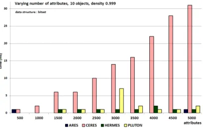
We illustrate typical cases, which are obtained with 100 attributes. With low densities (e.g 0.01, Figure 4) Ceres is the best algorithm. With high densities (e.g 0.999, Figure 5), Ares is often the best, sometimes challenged by Ceres. With medium densities (e.g 0.5, Figure6), Hermes and Pluton are the best, showing similar running time, Hermes being often better than Pluton.
Fig. 4: Varying the number of objects; 100 attributes; density = 0.01. Computation times are in milliseconds.
Fig. 6: Varying the number of objects; 100 attributes; density = 0.5
Observing all the figures, we infer that when the object number is much greater than the number of attributes, the better choices are:
– with medium densities: Hermes or Pluton – with low densities: Ceres
– with high density value: Ares or Ceres
Varying the number of attributes.
To study the effect of a variation in the number of attributes, as above, we consider three possibilities for the number of objects (10, 20 or 100). For each possibility, we evaluate several densities: {0.001, 0.01, 0.1, 0.2, 0.3, 0.4, 0.5, 0.6, 0.7, 0.8, 0.9, 0.99, 0.999}. In each density case, the number of attributes evolves from 500 to 5000.
We illustrate typical cases, which are obtained with 100 objects. With low densities (e.g 0.01, Figure 7) Ares is the best algorithm. With high densities (e.g 0.999, Figure 8), Hermes is the best algorithm. With medium densities (e.g 0.5, Figure 9 or Figure 10), Ceres or Hermes or Pluton are the best algorithms.
When the number of objects is very small, e.g. equals to 10 and density is very low (0.001) or very high (0.999), Ares becomes the best algorithm.
Observing all the figures, we infer that when the attribute number is much greater than the number of objects, the better choices are:
– with medium densities: Ceres, Hermes or Pluton – with low densities: Ares
– with high density value: Hermes (except when the number of objects is very small, cases where Ares is the best, then Hermes)
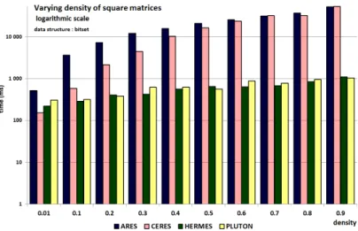
Square context with varying density.
Figure 12 (or Figure 13 with logarithmic scale) shows a typical situation with randomly generated square contexts (such that the number of rows is equal to the number of columns). With a low density (0.01), we do not notice a large difference between the four algorithms. But as the density grows, the gap between the running time of Ares and Ceres, on one side, and of Hermes and Pluton, on the other side, strongly increases. The running time of Hermes versus Pluton gives a slight advantage to Hermes. Furthermore, with very low densities (see Figure 14), which corresponds to the real cases that we found, Ceres is the best algorithm, followed by Hermes.
Fig. 7: Varying the number of attributes; 100 objects; density = 0.01
Fig. 8: Varying the number of attributes; 100 objects; density = 0.999
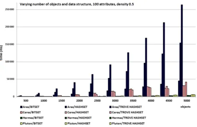
A.2 Effect of changing the data structures
As mentioned before, three alternative data-structures, BitSet, HashSet and TIntHashSet, have been used to examine what is the effect of the data-structure principle and implementation on the runtime. In most of the cases, the runtimes of the four algorithms keep the same relative positions: e. g. in Figure 15, Ares has the worst running time, followed by Ceres, then by Hermes and Pluton which have close running time. An alternative view is given with a logarithmic scale in Figure 16. But we can notice, in this representative example, that with the BitSet data-structure, the difference between Ares and Ceres is not as important as for the two other data-structures.
Fig. 9: Varying the number of attributes; 100 objects; density = 0.5
Fig. 10: Varying the number of attributes; 100 objects; density = 0.5, without
Ares
A.3 Results on real binary relations
We also applied the four algorithms with the three alternative data-structures to real binary relations, from several domains. Our first case study was composed of data extracted from three versions of the ArgoUML software: rows are various versions of the software (10 versions), while columns are source code elements (between 10 426 and 78 003) appearing in these versions (many were common to several versions), and density is about 0.95. It was interesting to notice in this case that the HashSet implementations were very bad for Hermes (e.g. in version 1, more than 175 sec), while the use of BitSet was good (e.g. in version 1, a few seconds). For this first case study, Pluton and Ares appear as good implementations. This dataset corresponds
Fig. 11: Varying the number of attributes; 10 objects; density = 0.999
Fig. 12: Results on square contexts (1000×1000)
to few objects, many attributes, and a high density, where we noticed, in the case of randomly generated data that Hermes, Pluton and Ares are the best.
Our second case study was a subset of source code elements of ArgoUML with a similarity relationship giving a square context (1505 objects and attributes) with a medium density (about 0.5). Pluton is always the best for this second case, followed by Ceres, and then Hermes, while in the randomly generated relations, Hermes then Pluton were the best.
Then we tested the implementations on eight binary contexts with different numbers of objects and attributes, square or almost square, with various dimensions and a very low density, taken from the Koblenz Network Collection. Figure 17a gives a representative example and typical results for the three data-structures: Ceres always is the best, followed by Hermes, then by Pluton. Figure17b (left hand side) recalls the bitset implementation results, and compares them with the results of the algorithms on randomly generated binary relations with
Fig. 13: Results on square contexts (1000×1000), log. scale
Fig. 14: Results on square contexts (2000×2000) and very low density.
same dimension and same density (right hand side of Figure 17b). The relative positions of the algorithms are the same.
For the first use case, with the ArgoUML dataset, which has a few objects, many attributes, and a high density, we notice that Hermes and Ares are the best (cf Fig 10). We have similar results for randomly generated data than for real data. For the second use case, where we have a square context and a medium density: the results are not significantly different between Pluton and Hermes. The dataset has a good profile for Ceres, with significant attribute group size, explaining its performance. For the other use cases, of which the open-fligth dataset is representative, as shows the Figure 14, the algorithms have different computation times, but their compared positions are the same.
Fig. 15: An example of the effect of using alternative data-structures.
(a) “Openflights” (b) Random
Fig. 17: Effects of the data structure on a representative real relation “Open-flights” (17a) and its comparison with random relation with same dimensions and density (17b). Square context “Openflights” is taken from http://konect.uni-koblenz.de/networks/opsahl-openflights. The BitSet implementation has been used in both relations.