Pépite | Utilisation de la microscopie à force atomique dans un contexte de mesures corrélatives multimodales et multi-échantillons sur cellules vivantes

Texte intégral

(1)Thèse de Antoine Dujardin, Université de Lille, 2018. Université de Lille. École Doctorale - 072 - Sciences Pour l’Ingénieur. Thèse de doctorat. Atomic Force Microscopy Usage in a Context of Multi-Mode and Multi-Sample Correlative Measures on Live Cells Bruker - CMPI. Antoine Dujardin Soutenue publiquement le 18 décembre 2018 en vue de l’obtention du grade de Docteur de l’Université de Lille spécialité Micro-Nanosystèmes et Capteurs M. Mme M. Mme Mme M. M.. © 2018 Tous droits réservés.. Tuami Lasri Touria Cohen-Bouhacina Grégory Francius Véronique Vie Andrea Slade Vincent Dupres Frank Lafont. Université de Lille Université de Bordeaux LCPME – CNRS Nancy Université de Rennes Bruker Nano Surfaces Université de Lille CMPI – CIIL (Lille). Président Rapporteur Rapporteur Examinateur Examinateur Superviseur Invité. lilliad.univ-lille.fr.

(2) Thèse de Antoine Dujardin, Université de Lille, 2018. Abstract Soon after its development in the late 1980s, atomic force microscopy (AFM) has shown promising applications in the biomedical field. It now allows investigating biological samples from single molecules to living cells under conditions close to physiological. Despite its applicability to both eukaryotic and prokaryotic cells, it is hampered by its low throughput. While heavily automated on some well-characterized samples in air, AFM automation in fluid is very scarce, especially at the multi-sample level. During this doctoral project, an automated approach was developed in fluid, on cells. After introducing the system and the developments required, we demonstrate the approach on fixed and living bacteria as well as on epithelial cells. The usage of multi-sample automation allows gathering a greater number of samples with limited user interaction. Finally, further developments are discussed to lead the path toward higher-scale AFM automation of live samples. Keywords Atomic Force Microscopy, PeakForce Tapping, Microbiology, Automation, Living cells, Multi-Sample.. ii. © 2018 Tous droits réservés.. lilliad.univ-lille.fr.

(3) Thèse de Antoine Dujardin, Université de Lille, 2018. Résumé Assez rapidement après son apparition à la fin des années 1980, la Microscopie à Force Atomique (AFM) a démontré des perspectives prometteuses d’applications biomédicales. À l’heure actuelle, elle permet l’étude d’échantillons biologiques allant de la molécule unique à la cellule vivante proche des conditions physiologiques. Bien qu’étant applicable aux cellules eucaryotes et procaryotes, elle est entravée par son faible débit. Alors qu’elle peut être fortement automatisée sur certains échantillons bien caractérisés en air, l’automatisation de l’AFM en liquide reste rare, en particulier en multi-échantillon. Lors de ce projet doctoral, une approche automatisée a été développée pour l’étude des cellules en milieu liquide. Après une introduction du système et des développements nécessaires, nous démontrons l’approche sur des bactéries fixées et vivantes, ainsi que sur des cellules épithéliales. L’utilisation d’automatisation multi-échantillon permet d’augmenter le nombre d’échantillons analysés tout en limitant les interactions avec l’utilisateur. Enfin, les développements ultérieurs sont discutés pour aller vers un système automatisé à plus grande échelle sur échantillons vivants. Mots-clés Microscopie à Force Atomique, PeakForce Tapping, Microbiologie, Automatisation, Cellules Vivantes, Multi-Échantillon.. iii. © 2018 Tous droits réservés.. lilliad.univ-lille.fr.

(4) Thèse de Antoine Dujardin, Université de Lille, 2018. Résumé Le but principal du travail présenté consiste en le développement d’un système de microscopie à force atomique (AFM) automatisé adapté à un usage multi-échantillon sur cellules vivantes. Il a été réalisé au sein du groupe de Microbiologie Cellulaire et Physique de l’Infection (CMPI) du Centre d’Infection et d’Immunité de Lille (CIIL). Ce projet est issu d’une convention CIFRE de l’ANRT avec l’entreprise Bruker. Le présent manuscrit, clôturant ce volet du projet, est séparé en deux parties rassemblant neuf chapitres. La première partie débute par une introduction détaillée de la microscopie à force atomique, au chapitre 2. Elle est alors suivie du chapitre 3, présentant des notions de biologie et des exemples d’applications de l’AFM dans ce domaine. Enfin, les défis actuels liés à ces applications sont présentés avec un état de l’art sur leurs solutions potentielles dans le chapitre 4. Ce dernier conclut sur l’importance d’augmenter le débit de l’AFM sur cellules. En effet, les mesures considérées n’ont de sens que sur un ensemble de cellules et la précision de celles-ci dépend du nombre de cellules prises en compte. Afin d’augmenter ce nombre, il y est montré la nécessité d’apporter de l’automatisation aux systèmes AFM, ainsi que l’avancée de la technologie dans ce domaine. La seconde partie de ce manuscrit présente donc un système permettant l’analyse multi-échantillon automatisée par AFM d’échantillons biologiques. Le chapitre 5 présente alors les impératifs d’un tel système. Ensuite, le chapitre 6 développe les bases de ce système d’un point de vue du matériel, d’un moteur de scripts et d’un outil d’analyse des données. Ces trois éléments clés mis en œuvre, l’automatisation en tant que telle peut être. iv. © 2018 Tous droits réservés.. lilliad.univ-lille.fr.

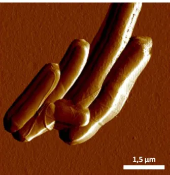
(5) Thèse de Antoine Dujardin, Université de Lille, 2018. développée. Ses particularités liées au type d’échantillons utilisé sont discutés au chapitre 7. Les problématiques liées à l’apparition de bulles d’air à proximité du levier, à la détection des cellules, ainsi qu’aux contaminations y sont discutées. Le fonctionnement du système est ensuite démontré au chapitre 8 sur le point de sa capacité à scanner de nombreuses cellules et entre plusieurs échantillons sur cellules procaryotes fixées Yersinia pseudotuberculosis. La démonstration est ensuite portée sur des cellules vivantes de type Mycobacterium bovis BCG. Finalement, le système est utilisé sur des cellules eucaryotes, issues de l’épithélium pigmentaire rétinien (RPE-1). Ensuite, des développements futurs sont étudiés et discutés dans le chapitre 9. Y sont discutés le contrôle de position des cellules, le changement de fluide, le contrôle en température et le contrôle qualité de la pointe. Pour terminer, le chapitre 10 rassemble la conclusion ainsi que les développements pressentis et suggérés à court, moyen et long terme. L’automatisation permet d’augmenter le nombre d’échantillons scannés, ce qui est nécessaire pour lever l’un des problèmes majeurs de l’AFM sur cellules vivantes : la faible signification statistique parfois rencontrée, limitant ainsi sa reproductibilité. La capacité du système à travailler en multi-échantillon permet aussi de limiter les variations d’un échantillon à l’autre, améliorant la comparabilité des résultats.. v. © 2018 Tous droits réservés.. lilliad.univ-lille.fr.

(6) Thèse de Antoine Dujardin, Université de Lille, 2018. Contents 1. Preface 1.1. Motivation . . . . . . . . . . . . . . . . . . . . . . . . . . . 1.2. Stakeholders . . . . . . . . . . . . . . . . . . . . . . . . . . 1.3. Structure of the Dissertation . . . . . . . . . . . . . . . . .. 1 1 2 3. I. Introduction. 5. 2. Atomic Force Microscopy 2.1. Operation . . . . . . . . . . . 2.1.1. Probe . . . . . . . . . 2.1.2. Tip . . . . . . . . . . . 2.1.3. Piezoelectric Actuators 2.1.4. Detection Mechanism . 2.2. Standard AFM Modes . . . . 2.2.1. Imaging Modes . . . . 2.2.2. Contact Mode . . . . . 2.2.3. Oscillating Modes . . . 2.2.4. Force Curves . . . . . 2.2.5. Force Volume . . . . . 2.3. AFM in Fluid . . . . . . . . . 2.3.1. Relevant Landmarks . 2.3.2. Sample Preparation . . 2.4. PeakForce . . . . . . . . . . . 2.4.1. Off-Resonance Tapping 2.4.2. Pseudo Force Curves . 2.4.3. Operation . . . . . . . 2.4.4. Hydrodynamic Effects 2.4.5. ScanAsyst . . . . . . . 2.5. Artifacts . . . . . . . . . . . . 2.5.1. Hysteresis and Creep . 2.5.2. Convolution . . . . . .. . . . . . . . . . . . . . . . . . . . . . . .. . . . . . . . . . . . . . . . . . . . . . . .. . . . . . . . . . . . . . . . . . . . . . . .. . . . . . . . . . . . . . . . . . . . . . . .. . . . . . . . . . . . . . . . . . . . . . . .. . . . . . . . . . . . . . . . . . . . . . . .. . . . . . . . . . . . . . . . . . . . . . . .. . . . . . . . . . . . . . . . . . . . . . . .. . . . . . . . . . . . . . . . . . . . . . . .. . . . . . . . . . . . . . . . . . . . . . . .. . . . . . . . . . . . . . . . . . . . . . . .. . . . . . . . . . . . . . . . . . . . . . . .. . . . . . . . . . . . . . . . . . . . . . . .. . . . . . . . . . . . . . . . . . . . . . . .. . . . . . . . . . . . . . . . . . . . . . . .. . . . . . . . . . . . . . . . . . . . . . . .. 6 8 8 10 12 15 16 16 17 18 19 23 25 25 26 28 28 29 31 32 34 35 35 37. vi. © 2018 Tous droits réservés.. lilliad.univ-lille.fr.

(7) Thèse de Antoine Dujardin, Université de Lille, 2018. Contents 2.5.3. Double Tip . . . . 2.5.4. Force Deformation 2.5.5. Parachuting . . . . 2.5.6. Sawtooth . . . . . 2.5.7. Horizontal Lines . . 2.5.8. Diagonal Stripes . 2.5.9. Other Artifacts . . 2.6. High-Speed AFM . . . . .. . . . . . . . .. . . . . . . . .. . . . . . . . .. . . . . . . . .. . . . . . . . .. . . . . . . . .. . . . . . . . .. . . . . . . . .. . . . . . . . .. . . . . . . . .. . . . . . . . .. . . . . . . . .. . . . . . . . .. . . . . . . . .. . . . . . . . .. . . . . . . . .. . . . . . . . .. 39 40 41 41 42 43 43 43. 3. Biology and Relevant Applications 3.1. The Cell . . . . . . . . . . . . . . 3.2. Eukaryotic Cells . . . . . . . . . . 3.2.1. Membrane . . . . . . . . . 3.2.2. Intracellular Components . 3.2.3. Extracellular Matrix . . . 3.2.4. Epithelial Cells . . . . . . 3.3. Prokaryotic Cells . . . . . . . . . 3.3.1. Cell Envelope . . . . . . . 3.3.2. Mycolata . . . . . . . . . 3.3.3. Model Samples . . . . . . 3.4. Understanding Diseases . . . . . . 3.4.1. Pathogens . . . . . . . . . 3.4.2. Drugs . . . . . . . . . . . 3.4.3. Antibiotics . . . . . . . . . 3.4.4. Antibiotic Resistance . . . 3.4.5. Cancer . . . . . . . . . . . 3.5. AFM Applications . . . . . . . . 3.5.1. Biological Conditions . . . 3.5.2. High-Resolution . . . . . . 3.5.3. Cell Mechanics . . . . . . 3.5.4. Single Cell Analysis . . . . 3.5.5. Monitoring . . . . . . . .. . . . . . . . . . . . . . . . . . . . . . .. . . . . . . . . . . . . . . . . . . . . . .. . . . . . . . . . . . . . . . . . . . . . .. . . . . . . . . . . . . . . . . . . . . . .. . . . . . . . . . . . . . . . . . . . . . .. . . . . . . . . . . . . . . . . . . . . . .. . . . . . . . . . . . . . . . . . . . . . .. . . . . . . . . . . . . . . . . . . . . . .. . . . . . . . . . . . . . . . . . . . . . .. . . . . . . . . . . . . . . . . . . . . . .. . . . . . . . . . . . . . . . . . . . . . .. . . . . . . . . . . . . . . . . . . . . . .. . . . . . . . . . . . . . . . . . . . . . .. . . . . . . . . . . . . . . . . . . . . . .. 45 45 46 48 49 52 52 52 53 56 57 60 61 61 61 62 63 64 65 66 66 69 70. . . . .. 73 74 75 77 79. 4. Challenges and Current Solutions 4.1. Trueness . . . . . . . . . . . . 4.1.1. Deflection Sensitivity . 4.1.2. Spring Constant . . . . 4.1.3. SNAP . . . . . . . . .. . . . . . . . .. . . . .. . . . .. . . . .. . . . .. . . . .. . . . .. . . . .. . . . .. . . . .. . . . .. . . . .. . . . .. . . . .. . . . .. . . . .. vii. © 2018 Tous droits réservés.. lilliad.univ-lille.fr.

(8) Thèse de Antoine Dujardin, Université de Lille, 2018. Contents 4.2. Precision . . . . . . . . . . . . . 4.2.1. Corresponding Problems 4.3. Faster Scanning . . . . . . . . . 4.3.1. Fixed Time . . . . . . . 4.3.2. Variable Time . . . . . . 4.4. Parallel Scanning . . . . . . . . 4.5. Unattended Scanning . . . . . . 4.5.1. Automated Steps . . . . 4.5.2. Automated Scan . . . . 4.5.3. Automated Systems . . .. . . . . . . . . . .. . . . . . . . . . .. . . . . . . . . . .. . . . . . . . . . .. . . . . . . . . . .. . . . . . . . . . .. . . . . . . . . . .. . . . . . . . . . .. . . . . . . . . . .. . . . . . . . . . .. . . . . . . . . . .. . . . . . . . . . .. . . . . . . . . . .. . . . . . . . . . .. . . . . . . . . . .. II. Results. 80 82 83 84 84 86 90 90 93 94. 98. 5. Objectives and Requirements 5.1. Requirements . . . . . . . 5.1.1. Scan . . . . . . . . 5.1.2. Correlation . . . . 5.1.3. Automation . . . . 5.1.4. Multi-Conditions . 5.1.5. Cell Survival . . . . 5.1.6. Work Hypothesis .. . . . . . . .. . . . . . . .. . . . . . . .. 6. Methodology 6.1. Multi-Well . . . . . . . . . . . . 6.1.1. Design . . . . . . . . . . 6.1.2. Sample Preparation . . . 6.1.3. Developments . . . . . . 6.2. Script Engine . . . . . . . . . . 6.2.1. Editor . . . . . . . . . . 6.2.2. Python Engine . . . . . 6.2.3. NanoScope Package . . . 6.3. Analysis Toolbox . . . . . . . . 6.3.1. Analysis Issue . . . . . . 6.3.2. Manufacturer Programs 6.3.3. Other Programs . . . . . 6.3.4. Direct Opening . . . . . 6.3.5. NS Python Toolbox . . .. . . . . . . . . . . . . . . . . . . . . .. . . . . . . . . . . . . . . . . . . . . .. . . . . . . . . . . . . . . . . . . . . .. . . . . . . . . . . . . . . . . . . . . .. . . . . . . . . . . . . . . . . . . . . .. . . . . . . . . . . . . . . . . . . . . .. . . . . . . . . . . . . . . . . . . . . .. . . . . . . . . . . . . . . . . . . . . .. . . . . . . . . . . . . . . . . . . . . .. . . . . . . . . . . . . . . . . . . . . .. . . . . . . . . . . . . . . . . . . . . .. . . . . . . . . . . . . . . . . . . . . .. . . . . . . . . . . . . . . . . . . . . .. . . . . . . . . . . . . . . . . . . . . .. . . . . . . .. 99 100 102 102 103 105 105 107. . . . . . . . . . . . . . .. 109 109 109 112 112 114 115 115 117 118 118 119 119 122 123. viii. © 2018 Tous droits réservés.. lilliad.univ-lille.fr.

(9) Thèse de Antoine Dujardin, Université de Lille, 2018. Contents. 7. Live Cell Automation 7.1. Specialized Scripting Tools . . . 7.1.1. Movement Control . . . 7.1.2. Experiment . . . . . . . 7.2. Issues and Solutions . . . . . . 7.2.1. Bubbles . . . . . . . . . 7.2.2. Cell Detection . . . . . . 7.2.3. Contamination Detection. . . . . . . .. . . . . . . .. . . . . . . .. . . . . . . .. . . . . . . .. . . . . . . .. . . . . . . .. . . . . . . .. . . . . . . .. . . . . . . .. . . . . . . .. . . . . . . .. . . . . . . .. . . . . . . .. . . . . . . .. 125 125 125 127 132 132 139 140. 8. Demonstration 8.1. Multi-Cells . . . . . . . . . 8.1.1. Sample Preparation 8.1.2. Setup . . . . . . . 8.1.3. Results . . . . . . . 8.2. Multi-Conditions . . . . . 8.2.1. Sample Preparation 8.2.2. Analysis . . . . . . 8.2.3. Results . . . . . . . 8.2.4. Conclusion . . . . . 8.3. Living Cells . . . . . . . . 8.4. Eukaryotes . . . . . . . .. . . . . . . . . . . .. . . . . . . . . . . .. . . . . . . . . . . .. . . . . . . . . . . .. . . . . . . . . . . .. . . . . . . . . . . .. . . . . . . . . . . .. . . . . . . . . . . .. . . . . . . . . . . .. . . . . . . . . . . .. . . . . . . . . . . .. . . . . . . . . . . .. . . . . . . . . . . .. . . . . . . . . . . .. . . . . . . . . . . .. 141 141 141 142 142 146 147 147 151 153 153 154. . . . . . . . . . . .. 162 162 163 163 165 165 165 166 166 168 171 175. . . . .. 181 181 184 184 186. . . . . . . . . . . .. . . . . . . . . . . .. . . . . . . . . . . .. 9. Further Developments 9.1. Controlling Cells Position . . . . . . . . . . . 9.1.1. Chemical Binding on Mammalian Cells 9.1.2. Chemical Binding on Bacteria . . . . . 9.1.3. Physical Confinement on Bacteria . . . 9.1.4. Hybrid Systems . . . . . . . . . . . . . 9.1.5. Interest . . . . . . . . . . . . . . . . . 9.2. Fluid Exchange . . . . . . . . . . . . . . . . . 9.2.1. Fluid Evaporation . . . . . . . . . . . 9.2.2. Implementation . . . . . . . . . . . . . 9.3. Heating . . . . . . . . . . . . . . . . . . . . . 9.4. Tip Control . . . . . . . . . . . . . . . . . . . 10.Conclusion and Future Outlook 10.1. Conclusion . . . . . . . . . . 10.2. Future Outlook . . . . . . . 10.2.1. Short Term . . . . . 10.2.2. Medium Term . . . .. . . . .. . . . .. . . . .. . . . .. . . . .. . . . .. . . . .. . . . .. . . . .. . . . .. . . . . . . . . . . . . . . .. . . . . . . . . . . . . . . .. . . . . . . . . . . . . . . .. . . . . . . . . . . . . . . .. . . . . . . . . . . . . . . .. . . . . . . . . . . . . . . .. ix. © 2018 Tous droits réservés.. lilliad.univ-lille.fr.

(10) Thèse de Antoine Dujardin, Université de Lille, 2018. Contents 10.2.3. Long Term . . . . . . . . . . . . . . . . . . . . . . .. Appendix. 187. 191. A. Protocols A.1. Consumables . . . . . . . . A.2. Coverslip Pre-Treatment . . A.3. Yersinia pseudotuberculosis . A.3.1. Culture . . . . . . . A.3.2. Treatment . . . . . . A.3.3. Plating . . . . . . . . A.4. Mounting . . . . . . . . . . A.5. Default Setup . . . . . . . .. . . . . . . . .. 191 191 191 191 191 192 192 192 193. B. Accuracy B.1. Precision . . . . . . . . . . . . . . . . . . . . . . . . . . . . B.2. Trueness . . . . . . . . . . . . . . . . . . . . . . . . . . . . B.3. Accuracy . . . . . . . . . . . . . . . . . . . . . . . . . . . .. 195 195 196 196. C. Models C.1. Contact Models . . . . . . . C.1.1. Elastic Models . . . C.1.2. Hertz . . . . . . . . . C.1.3. Sneddon . . . . . . . C.1.4. Adhesive Models . . C.1.5. Thin Samples . . . . C.2. Tomography . . . . . . . . . C.2.1. Stiffness Tomography C.3. Contact Point . . . . . . . .. . . . . . . . . .. 198 198 199 200 201 201 202 202 202 203. . . . . .. 205 205 205 206 207 207. E. Developments Summary E.1. Biological Medium . . . . . . . . . . . . . . . . . . . . . .. 209 209. . . . . . . . .. . . . . . . . . .. . . . . . . . .. . . . . . . . . .. D. Computing Science D.1. Dynamic Link Libraries . . . . D.2. .NET . . . . . . . . . . . . . . . D.3. Python . . . . . . . . . . . . . . D.3.1. IronPython . . . . . . . D.4. IronPython to CPython Bridge. . . . . . . . .. . . . . . . . . . . . . . .. . . . . . . . .. . . . . . . . . . . . . . .. . . . . . . . .. . . . . . . . . . . . . . .. . . . . . . . .. . . . . . . . . . . . . . .. . . . . . . . .. . . . . . . . . . . . . . .. . . . . . . . .. . . . . . . . . . . . . . .. . . . . . . . .. . . . . . . . . . . . . . .. . . . . . . . .. . . . . . . . . . . . . . .. . . . . . . . .. . . . . . . . . . . . . . .. . . . . . . . .. . . . . . . . . . . . . . .. . . . . . . . .. . . . . . . . . . . . . . .. . . . . . . . .. . . . . . . . . . . . . . .. . . . . . . . .. . . . . . . . . . . . . . .. . . . . . . . .. . . . . . . . . . . . . . .. x. © 2018 Tous droits réservés.. lilliad.univ-lille.fr.

(11) Thèse de Antoine Dujardin, Université de Lille, 2018. Contents. E.2. E.3. E.4. E.5. E.6. E.7. E.8.. Biocompatibility . . . Limited Handling . . . Environmental Control Light and Visibility . . Immobilization . . . . Fluid Exchange . . . . Suitability for Cells . .. . . . . . . .. . . . . . . .. . . . . . . .. . . . . . . .. . . . . . . .. . . . . . . .. . . . . . . .. . . . . . . .. . . . . . . .. . . . . . . .. . . . . . . .. . . . . . . .. . . . . . . .. . . . . . . .. . . . . . . .. . . . . . . .. . . . . . . .. . . . . . . .. . . . . . . .. . . . . . . .. 209 210 210 211 212 212 213. xi. © 2018 Tous droits réservés.. lilliad.univ-lille.fr.

(12) Thèse de Antoine Dujardin, Université de Lille, 2018. 1. Preface 1.1. Motivation Bacterial resistance to antibiotics are a major health-care issue as the pharmaceutical industry fails to keep up with the production of new drugs to compensate for the obsolescence of the current ones. Therefore, approaches other than a direct targeting of the pathogen are required, such as the study of the host-pathogen interactions in order to act on the mechanisms of the host. Shifting the targeting from the pathogen to its interactions with the host would bypass the currently existing pathogen resistances and could consequently be of great use against multi-resistant strains. An understanding of these interactions can come from their comparison with and without gene editing or drug injection, which can be performed by screening techniques. Basic screening techniques have a single color per well depending on the viability of the cell. It yields a unidimensional “color” signal for each well, which is a very limited, almost binary, information for each drug-host-pathogen triplet. They can, however, be recorded very quickly. These very-high-throughput but low-content techniques could, therefore, only be used in the very first step of the screening process, where the throughput has to be maximized in order to keep a few hits for the subsequent, higher content but lower throughput techniques. High Content Screening with super-resolution imaging techniques can then be performed in order to gain more information of the combinations of interest while keeping a relatively high throughput. Afterward, the new hits can be studied further with higher-content tech-. 1. © 2018 Tous droits réservés.. lilliad.univ-lille.fr.

(13) Thèse de Antoine Dujardin, Université de Lille, 2018. 1. Preface. niques, such as Atomic Force Microscopy, Electron Microscopy, or other kinds of super-resolution microscopy. These techniques, offering the highest resolution imaging along with information on the local compositions or properties, are however much more operation intensive. They suffer, as a consequence, from a much slower throughput. It is especially the case for Atomic Force Microscopy, which is therefore still very uncommon in the study of microbiology and pathogeny. Correlative setups, merging together two or more of the techniques mentioned above, can bring the most quantitative and qualitative information on a microbiological system, at the expense of being prohibitively slow. Therefore, we focused our work on the development of biomedicallyrelevant tools and applications for Atomic Force Microscopy that are centered around multi-sample analysis. During the three years leading to this thesis were developed innovative hardware, software, and methodological solutions for the sake of bringing Atomic Force Microscopy on Live Cells from a very low throughput to a medium one. Aside from pointing towards a high-content technique as mentioned above, such improvements can have a shorter-term positive impact on simply improving the statistical significance of AFM studies, which is one of its current shortcomings.. 1.2. Stakeholders This project was sponsored by France’s National Association for Research and Technology (ANRT) under an Industrial Agreement of Training through Research (CIFRE) Program between a laboratory, the CMPI, and a company, Bruker. The CMPI—the Cellular Microbiology and Physics of Infection group—investigates host-pathogen interactions in the realm of infectious diseases, in particular regarding the autophagy activation as a response to infection. It uses a multidisciplinary approach based on AFM and super-resolution microscopy with a focus on the elastic properties of cells. The CMPI research group is part of the Center for Infection and Immunity. 2. © 2018 Tous droits réservés.. lilliad.univ-lille.fr.

(14) Thèse de Antoine Dujardin, Université de Lille, 2018. 1. Preface. of Lille, on the campus of the Pasteur Institute of Lille, France. Bruker, on the other hand, is a high-performance scientific instruments manufacturer, operating mostly on molecular-scale technologies. It possesses, in particular, a great expertise in the manufacturing and development of Atomic Force Microscopes at its facilities in Santa Barbara, California, U.S.A, where parts of this project were carried out. As a joint venture between the two, this work benefited from both of their means and expertise.. 1.3. Structure of the Dissertation Part I of the dissertation will give an introductory overview, introducing Atomic Force Microscopy (Chapter 2) followed by biology and the corresponding applications (Chapter 3). Afterwards, we will discuss the ongoing challenges of AFM on biological matter and review existing solutions (Chapter 4). In particular, we will see the importance of sample sizes and develop on the necessity of going towards a multi-sample system. In Part II, we will then describe a system developed to detect and scan cells autonomously. This leads us towards higher-throughput applications related to the biomedical, pharmaceutical, and other health-related fields. We will first go through the requirements of such a system in the section below before presenting our setup. This system is composed of a MultiWell for the hardware as well as a script engine and a data analysis toolbox for the software, which are the basic methodological elements described in Chapter 6. Based on these elements, a range of domain-specific scripts have been developed for the general workflow and to solve specific issues, the topic of Chapter 7. This system is then demonstrated in Chapter 8 on multiple cells of a sample and on multiple samples on fixed cells, then shown to be applicable to live cells and eukaryotic ones. After that, Chapter 9 introduces potential further developments for which proofs of concepts have been developed but not integrated into the main system. Chapter 10 finally closes the. 3. © 2018 Tous droits réservés.. lilliad.univ-lille.fr.

(15) Thèse de Antoine Dujardin, Université de Lille, 2018. 1. Preface. dissertation with the conclusion and a discussion on the path towards the desired high-content medium-throughput system.. 4. © 2018 Tous droits réservés.. lilliad.univ-lille.fr.

(16) Thèse de Antoine Dujardin, Université de Lille, 2018. Part I. Introduction. 5. © 2018 Tous droits réservés.. lilliad.univ-lille.fr.

(17) Thèse de Antoine Dujardin, Université de Lille, 2018. 2. Atomic Force Microscopy The fields of biology and medicine would still be far behind if it was not for the microscope, as microorganisms are too small for the human eye to see. Crude lenses having existed since antiquity, microscopy appeared as such in the seventeenth century, with Antonie van Leeuwenhoek, who built the first prototypes of optical microscopes, allowing him to observe the first unicellular organisms. Nowadays, this flavor of microscopy is still considered as an entry-point to the observation of microorganisms, as its functioning is close to the way our vision works, making it easier to interpret for the untrained eye. Optical microscopy improved over time, allowing for high-resolution imaging, until reaching resolutions no longer limited by the quality of the optics but by a fundamental behavior of light: diffraction. Light, as a wave, is characterized by its wavelength (λ) and interacts in such a way that it loses its intuitive ray-like properties when the resolution approaches the scale of the wavelength. It is not possible to resolve elements smaller than about λ/2, which corresponds to a limit at 200 nm for visible light. This can be overcome by using waves of higher frequencies, such as X-rays. A higher frequency is, however, related to a higher energy, causing consequent harm to the sample. Fluorescence microscopy overcomes some of these limitations by the use of fluorescent probes that specifically bind to elements of interest. While the resolution limit is still the same, it alleviates the need of recognizing the elements of interest in the image, the whole resolution being then used to detect their position, and sometimes structure. Furthermore, if the fluorescent probes are scarce enough to appear as separated dots in. 6. © 2018 Tous droits réservés.. lilliad.univ-lille.fr.

(18) Thèse de Antoine Dujardin, Université de Lille, 2018. 2. Atomic Force Microscopy. the image, their location can be algorithmically recovered with a resolution an order of magnitude better, which is the base of the PALM and STORM techniques. Rather than using an algorithmic reconstruction, other methods use an extremely localized illumination scheme to push the resolution bellow the diffraction limit, as done initially in confocal and then STED microscopy. Still, the highest resolution is limited to several tens of nanometers, whereas many biological processes—especially in the realm of interactions between cells (prokaryotes and eukaryotes alike) or with their environment—happen at the nanometric scale. The introduction of the scanning electron microscope (SEM) and the transmission electron microscope (TEM) allowed sub-nanometric resolution, creating therefore another breakthrough in the study of surfaces. The electron microscope, created by Ruska and Knoll in 1931, uses electrons deflected by magnetic coils acting as electromagnetic lenses, thanks to the wave properties of particles. Electron having a wavelength hundreds of thousands of times smaller than photons, they allow for such a better resolution. While allowing huge advances in our understanding of biological processes, electron microscopy requires fixing an contrasting the sample. It is, therefore, not suitable to image living samples. Both optical and electronic microscopies mentioned above use a beam (of photons or electrons) going from a source to a detector via a sample. Because of the distance separating the sample and the detector, these are considered as “far-field” microscopes. In the eighties came the scanning tunneling microscope (Binnig, Rohrer, et al., 1982), first of the scanning probe microscopes, which act on a completely different paradigm in that a measurement is taken at the local level with a probe extremely close to the sample. This paradigm belongs to the realm of “near-field” microscopy, which removes the problem of the diffraction limit all together. In the case of the STM, a voltage difference is applied between the sample and the tip, which creates a tunneling current. While raster-scanning the sample, the tip moves up and down to keep the tunneling current constant. The STM requires, however, to work on a conducting sample, which is. 7. © 2018 Tous droits réservés.. lilliad.univ-lille.fr.

(19) Thèse de Antoine Dujardin, Université de Lille, 2018. 2. Atomic Force Microscopy. Figure 2.1.: AFM probe, composed of a tip at the end of a cantilever attached to a chip. Both a rectangular (right) and a V-shaped (left) cantilevers are represented. © Bruker, modified.. quite restrictive. This constraint led to the development of the AFM (Binnig, Quate, and Gerber, 1986), which uses the force between the sample and the probe at the atomic level, removing the need for a current and thus bringing the possibility of working on non-conducting surfaces. The probe, in this case, is composed of a tip mounted on a flexible cantilever, which act as a spring when touching the sample. Atomic-scale AFM appeared less than a year later (Binnig, Gerber, et al., 1987). AFM is now used for R&D purposes on a lot of disciplines. These include solid-state physics, electro and polymer chemistry, as well as molecular and cell biology. It is also used for calibration purposes and quality control in the semiconductor and instrumentation industry.. 2.1. Operation The AFM is essentially composed of a probe, a sample, and a system to control and measure their relative movements. In a first time, we will assume here a hard macroscopic sample, unless otherwise specified.. 2.1.1. Probe The probe, illustrated in Figure 2.1, is made of a cantilever at the end of which lies a tip. Both are most often microfabricated from silicon nitride. 8. © 2018 Tous droits réservés.. lilliad.univ-lille.fr.

(20) Thèse de Antoine Dujardin, Université de Lille, 2018. 2. Atomic Force Microscopy. or silicon. The cantilever is bonded to a millimeter chip, or substrate, to allow easy handling and its attachment to the system. Cantilevers are usually long, thin rectangular beams or composed of two beams making a V shape. When a perpendicular force is applied at its end, the cantilever acts like a spring. It follows Hooke’s law, which states that the vertical displacement of the end of the beam (or deflection, d) and the applied force (F ) follow a constant ratio, named the spring constant (k): F = k × d. (2.1) In this document, we will consider the force and the deflection as positive when directed upwards. Aside from their spring constant, cantilevers are characterized by their resonant frequency ν0 . Both of these physical properties depend on the shape and the dimensions of the cantilever as well as the mechanical properties of the materials used for its fabrication, leading to a diversity in cantilever shapes and dimensions. In particular, for a rectangular cantilever with a constant rectangular cross-section, we have: Ewt3c k= 4L3 and. tc ν0 = 0.1615 2 L. (2.2). s. E , ρ. (2.3). where w is width of the cantilever, tc its thickness, L its length, with E and ρ being respectively the Young’s modulus and the density of its material. Nonetheless, small variations—especially on the thickness—can have a strong effect on the resulting properties, making the use of these formula unpractical for calibration purposes. Typical dimensions of the beams are 100 µm to 200 µm for the length, 20 µm to 40 µm for the width, and 0.5 µm to 1 µm for the thickness (Butt, Cappella, and Kappl, 2005). One may note that both the spring constant and the resonant frequency increase with E and tc and decrease with L. These two parameters tend,. 9. © 2018 Tous droits réservés.. lilliad.univ-lille.fr.

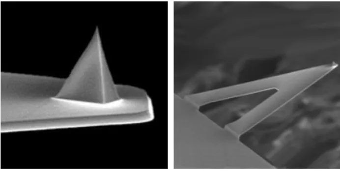
(21) Thèse de Antoine Dujardin, Université de Lille, 2018. 2. Atomic Force Microscopy. therefore, to correlate positively. Soft cantilevers are, however, required to avoid deforming or damaging the sample when imaging while a low resonant frequency of the cantilever limits the scanning speed. The requirement for soft cantilevers with high resonant frequencies for rapid applications led then to the design of particular cantilever geometries. For example, very small but comparatively soft cantilevers are used for highspeed applications. As we will see in Section 2.2.4, the spring constant is further constrained for nanomechanical measurement, where the stiffness of the cantilever and the sample should be similar. There might be more than one cantilever on the substrate, although only one can be used at a time. The chip, along with the cantilever, is tilted forward with an angle usually ranging from 7° to 20° to allow the tip to be slightly below the rest of the probe. It allows for the tip to be the first element to get in contact with the sample when lowered to it, as described further below.. 2.1.2. Tip The tip, shown in Figure 2.2, is the centerpiece of the instrument, as it is directly in contact with the sample. Its shape determines the resolution of the image (Abraham, Batra, and Ciraci, 1988), which is a “convolution”∗ of the object surface by the shape of the tip. As a consequence, the ideal tip shape for image resolution would be an infinitely thin and sharp tip at an angle compensating the tilt of the probe so that it touches the sample vertically. Even though carbon nanotube tips following that design have been developed in labs and used for highresolution imaging of fixed cells (Koehne et al., 2011), it is not usable in practice as they are extremely brittle and can pierce through soft matter. A more common tip shape is a pyramid with a deltoid base, which can be microfabricated with steep angles and where the end can be further ∗. It is actually not equivalent to a mathematical convolution, but this will be discussed in Section 2.5.2.. 10. © 2018 Tous droits réservés.. lilliad.univ-lille.fr.

(22) Thèse de Antoine Dujardin, Université de Lille, 2018. 2. Atomic Force Microscopy. Figure 2.2.: ScanAsyst-Fluid probe. Scanning Electron Microscopy images of the tip (left) and cantilever (right), taken upside down. © Bruker.. sharpened by etching. While less brittle, the sharpness of this design is still unsuitable for scanning live cells. When measuring the mechanical properties of locally homogeneous and flat materials, large and well-characterized shapes are needed. The resulting data can then be analyzed by fitting it to a contact model, such as described in Appendix C.1, most of which being based on the Hertz model (Hertz, 1882). Such shapes include the square pyramid, sphere, paraboloid, cone, or cylinder, usually with dimensions ranging from one to a few micrometers at their base. Spherical tips, or colloidal probes, usually have a diameter ranging from 2 µm to 20 µm and have particularly well-characterized models (Butt, Cappella, and Kappl, 2005). For applications where the mechanical properties are recorded locally to form a nanomechanical “image” of the sample, a trade-off has to be found between the locality of the probe and its characterization. Some well-characterized shapes such as the square pyramid and the cone might be suitable under certain conditions while spherical and cylindrical are inadequate for imaging. More complex tip geometries can then be used, such as diamond-shaped ones with a spherical cap end to allow both a high resolution and a good characterization. Although it is often made out of the same material as the cantilever,. 11. © 2018 Tous droits réservés.. lilliad.univ-lille.fr.

(23) Thèse de Antoine Dujardin, Université de Lille, 2018. 2. Atomic Force Microscopy. Figure 2.3.: Piezo extension and retraction, depending on the applied voltage. © Bruker.. other materials can be used for specific applications. As an example, diamond tips are often used on very hard samples. Tips are characterized by their tip radius, which ranges from less than 1 nm in the case of atomically sharp probes to 20 µm for colloidal probes.. 2.1.3. Piezoelectric Actuators High-resolution scanning is made possible by the use of piezoelectric translators, also called positioners, scanners, or actuators, usually named piezos. Thanks to their atomic structure, piezoelectric materials have the property of changing their shape depending on a voltage applied to their extremities. The actuators are made by placing electrodes on two opposites sides of the material and applying a voltage difference between the two. Depending on the orientation of the voltage difference, the piezo will contract or retract along the corresponding axis (here, the vertical one). A relation can be established between the relative displacement and the voltage difference, although it is affected by hysteresis and creep, which have to be controlled, minimized, and/or taken into account by the controller and the software. The piezos have the opposite movement in the two other axes (here, the horizontal and out-of-plane axis). In the case shown in Figure 2.3, applying a positive voltage on the top electrode will. 12. © 2018 Tous droits réservés.. lilliad.univ-lille.fr.

(24) Thèse de Antoine Dujardin, Université de Lille, 2018. 2. Atomic Force Microscopy. contract the piezo vertically and expend it horizontally whereas a negative voltage will have the opposite effect. Several piezos are used to control the movement of the probe relative to the sample in the X, Y, and Z direction. The X and Y scanners control the movements parallel the plane of the sample, whereas the Z one is perpendicular. Since only their relative positions matter, the scanners can either be placed to actuate the tip or the sample. In the Dimension FastScan AFM, used for most of the work presented further, the three scanners control the tip. Some other systems, however, have the horizontal (X-Y) or all scanners controlling the sample. Because of the complexity of the non-linear relation between the voltage and the displacement, it is difficult to blindly control the position of the tip with a great confidence. Thankfully, the piezoelectric effect can also generate a voltage difference from a displacement and can, as such, bring us to piezoelectric sensors. A first application of these sensors is to record the actual displacement and take it into account in the analysis. With sufficiently fast electronics, however, it is possible to use the measurement as a feedback to correct the applied voltage in real-time in what is known as “closed loop”. In this configuration, the actuators, the probe, the sample, and the optical lever are connected with a feedback circuit, represented in Figure 2.4. A controller records the deflection signal from the microscope and processes it. It then controls the (vertical) Z piezo actuator to keep the deflection at a certain setpoint. It should be noted that, while allowing a better control of the position, this technique can introduce some additional noise in the system. When properly calibrated, piezoelectric actuators and sensors can perform or record displacements with precisions of the order of the Ångström (1 Å = 0.1 nm).. 13. © 2018 Tous droits réservés.. lilliad.univ-lille.fr.

(25) Thèse de Antoine Dujardin, Université de Lille, 2018. 2. Atomic Force Microscopy. Figure 2.4.: Feedback loop. As the X and Y piezos are raster-scanned on the sample, the cantilever motion is continuously compared to a setpoint to correct the position of the vertical Z piezo, realising the data. © Bruker.. Figure 2.5.: Optical lever system. A laser is bounced on the back of the cantilever and targeted on a four-quadrants photodetector. A deflection of the cantilever, here due to the substrate, creates a displacement of the laser spot on the detector. © Bruker. 14. © 2018 Tous droits réservés.. lilliad.univ-lille.fr.

(26) Thèse de Antoine Dujardin, Université de Lille, 2018. 2. Atomic Force Microscopy. 2.1.4. Detection Mechanism As described above, the tip is mounted on the end of a long thin cantilever. Interaction forces between the sample and the tip will induce a deflection of the cantilever, which, on most current AFMs, is recorded by an optical lever system by means of a laser beam. This laser beam is pointed on the back of the cantilever with a vertical incidence, close to the position of the tip. The back of the cantilever is often coated with metal, such as gold or aluminum, to improve its reflectivity. As shown in Figure 2.5, the cantilever reflects the beam towards a photodetector composed of four photodiodes, which translate the intensity of light they receive into a voltage. The laser is originally aligned to fall in the center of the photodetector, with an equivalent coverage of all the photodiodes so that they all output similar voltages. In practice, mirrors are used to align the elements of the optical lever without moving them physically. Lenses and other optics are also used to better focus the laser spot on the cantilever. The laser source, the cantilever, and the photodetector form an optical lever. Assuming small displacements, the deflection of the cantilever will change the bending angle proportionately. The vertical incidence of the laser makes it close to perpendicular to the cantilever so that the laser spot stays at the same position, reflecting it towards the photodetector proportionally. Therefore, the position of the laser spot on the photodetector changes linearly with the deflection. In the pictured case, the cantilever and the beam are deflected upwards, increasing the intensity of light received by diodes A and B and decreasing the one received by C and D proportionately. The ratio dV =. A+B , A+B+C +D. (2.4). is then directly proportional to the deflection and usually assimilated as such and considered as the deflection “in Volts”. This value, along with. 15. © 2018 Tous droits réservés.. lilliad.univ-lille.fr.

(27) Thèse de Antoine Dujardin, Université de Lille, 2018. 2. Atomic Force Microscopy. the signal from the Z sensor, is recorded by the controler and sent to the computer, where it can be processed as developed below, displayed as an image or curves, and saved. The relationship between the deflection in distance units d and this value can be expressed as: d = ds × dV , (2.5) where ds is the deflection sensitivity, a constant that is measured during the calibration of the system. To record the vertical deflection of the cantilever, two photodiodes would suffice, merging A-B and C-D. Splitting the photodetector into four quadrants allows, however, better centering the laser spot at its center. The difference in laser intensity between the two left segments and the two right ones allows us to record a horizontal signal, which quantifies any lateral or twisting motion of the tip that can be used for recording friction. The first AFMs, however, used a method based on the scanning tunneling microscope. Essentially, the tip and cantilever were simply a “mobile coating” of the sample. Rather than coating the sample before scanning it with the STM, a tip and cantilever were added to the end of the STM. When being in contact with the sample, the cantilever acted like the metallic coating allowing the tunneling effect while keeping the sample intact.. 2.2. Standard AFM Modes 2.2.1. Imaging Modes During imaging modes, the feedback loop is used to adapt the tip position to the height of the sample in order to keep constant the interactions between the two. The tip is raster-scanned on the sample, usually with a fast linear movement along one axis, called the fast axis. As represented in Figure 2.6, this movement is repeated back and forth while a slow linear movement along the other, slow axis is performed. The back and forth. 16. © 2018 Tous droits réservés.. lilliad.univ-lille.fr.

(28) Thèse de Antoine Dujardin, Université de Lille, 2018. 2. Atomic Force Microscopy. Figure 2.6.: Raster-scan motion. The probe and the sample are scanned against each other along one axis, the fast scan direction, while moving at a slower pace along the slow scan axis, or direction. © Bruker. movements along the fast axis are called “trace” and “retrace”, respectively. The image obtained correspond to the topography of the sample, plus a “convolution” of the tip shape, the deformation of the sample caused by the scanning, and instabilities in the feedback system, among others common artifacts described below.. 2.2.2. Contact Mode As a simple application of a feedback loop on the deflection of the cantilever, contact mode (Hansma, Elings, et al., 1988) is the earliest imaging mode of AFM. It raster-scans the tip over the sample while adjusting the height to keep the cantilever deflection (hence the force) at the user-defined setpoint. It usually generates two images: the vertical position of the piezo at each X-Y position, and the deflection error (i.e. the difference between the deflection and the setpoint). If the deflection error is small, the piezo height map gives the sample topography, considering the artifacts described below. A strong disadvantage of contact mode is that it can also deform or displace the sample by the strong lateral forces due to the friction of the tip on the surface. If the fast axis is taken perpendicular to the cantilever, the cantilever can. 17. © 2018 Tous droits réservés.. lilliad.univ-lille.fr.

(29) Thèse de Antoine Dujardin, Université de Lille, 2018. 2. Atomic Force Microscopy. be twisted laterally by the friction forces opposing the movement of the tip on the sample. This movement translates to a horizontal displacement of the laser reflection on the photodetector, which can be recorded as a third set of data. Contact Mode can also be used at constant height, where the deflection is recorded but not used as feedback for the piezo extension. It can allow higher scan speeds since there is no need for feedback. It is, however, restricted to very flat samples, which strongly limits its applications in biology.. 2.2.3. Oscillating Modes As the constant contact between the tip and the sample generates strong shear constraints on the latter, intermittent contact and non-contact modes were developed shortly after. The vertical piezo (or a dedicated extra piezo) is oscillated close to the resonant frequency of the cantilever. Thanks to the resonance effect, the oscillation of the end of the cantilever is much bigger than the oscillation applied at its base by the piezo, the ratio between the two being the Qfactor. The cantilever is bent upward and downward at that frequency, creating oscillation of the deflection as recorded by the photodetector. The idealized case only works in vacuum, however, with Q-factors ranging from 104 to 108 although its use in air is very close and quite simple, with still decent Q-factors ranging on the order of 10 to 200. The resonance in fluid, on the other hand, is strongly affected by the fluid drag, which makes the technique much more challenging as the Q-factors can be much smaller than 1 (Butt, Cappella, and Kappl, 2005). The effective resonance frequency of the cantilever and the Q-factor depend, however, on the forces applied to the tip. As a consequence, recording shifts in amplitude, phase, or frequency can inform about changes in these forces due to the proximity of the sample. By enabling a feedback loop on one of these channels, one can generate a topography image in a similar. 18. © 2018 Tous droits réservés.. lilliad.univ-lille.fr.

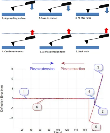
(30) Thèse de Antoine Dujardin, Université de Lille, 2018. 2. Atomic Force Microscopy. fashion as in contact mode. Martin, Williams, and Wickramasinghe (1987) developed the first noncontact technique, where the tip was oscillated with an amplitude of up to 5 nm close to the surface. In the presence of non-contact interactions, such as the attractive van der Waals force when working close to the atomic scale, a force gradient exists close to the surface. This gradient modifies the amplitude of the oscillation, which is used for the feedback. Although it presents the advantage of not touching the sample, hence not damaging it at all, non-contact mode only works within a narrow range of tip-sample distances. When the tip gets too close to the sample, it sticks to it and the scanning is blocked. Zhong et al. (1993) then introduced a similar concept of intermittent contact on amplitude modulation, or tapping mode, where the amplitude is much larger, typically between 20 and 100 nm. Intermittent contact with the sample allows the tip to move while not in direct contact with the sample, thus virtually eliminating the shear stress.. 2.2.4. Force Curves Contact and oscillating modes are interesting to explore the topography of a sample. Alternatively, rather than raster-scanning the sample along the horizontal axes while updating the vertical position to track the sample surface, one might want to focus on a given horizontal position and observe the reactions of the sample as it is probed. To do so, the probe starts at a position above the surface and is lowered by the Z piezo towards the sample. At some point, the probe gets in contact with the sample and the repulsive forces applied to the tip increase until the deflection of the cantilever reaches a threshold (or trigger). This triggers the retraction of the Z piezo to an elevated position. The downward movement is called the approach or extension, the upward one is the retraction. During both the approach and the retraction, the deflection of the cantilever and the vertical position of the piezo are recorded. Recording the deflection as shown in Equation (2.5) and using Hooke’s. 19. © 2018 Tous droits réservés.. lilliad.univ-lille.fr.

(31) Thèse de Antoine Dujardin, Université de Lille, 2018. 2. Atomic Force Microscopy. Figure 2.7.: Force curve. Left: path of the cantilever. Right: corresponding force curve. 1: non-contact approach. 2: snap-in contact. 3: trigger force. 4: zero-force contact. 5: maximum adhesion force (snap-off contact). 6: non-contact retraction. © Bruker, modified.. 20. © 2018 Tous droits réservés.. lilliad.univ-lille.fr.

(32) Thèse de Antoine Dujardin, Université de Lille, 2018. 2. Atomic Force Microscopy. law given in Equation (2.1), one can deduce the vertical force exerted on the tip once the deflection sensitivity and the spring constant have been calibrated. Knowing the force as a function of the distance during the approach and retract phases can release Force versus Distance (or Force-Distance) relationships such as the one presented in Figure 2.7 that, once analyzed, can give quantitative information on mechanical properties (Butt, Cappella, and Kappl, 2005; Cappella and Dietler, 1999). This distance is, however, the displacement of the probe as measured from the piezo and does not equate to the distance between the tip and the sample, which also depends on the deflection of the cantilever. Let this distance be Z = Z0 − dp , (2.6) where Z0 is the distance between the tip and the sample at the beginning of the approach, assuming no deflection of the cantilever nor the sample, and dp the piezo displacement from the upper position. As dp increase, Z decreases from Z0 to 0 and will reach negative values when the piezo is extended past the contact point. In this case, the tip-sample distance D can be expressed as D = Z + d + δ,. (2.7). where δ is the indentation of the sample, as represented in Figure 2.8. When the tip and the sample are well separated, the deflection and the indentation are null and the distance equals the displacement: d = δ = 0 and D = Z. Once the tip is in contact with the sample, at the scales used on cells (hence neglecting the variation in the interatomic distances), D = 0, and any further decrease in Z is balanced by an equivalent increase shared between d and δ. On an elastic sample and assuming equilibrium, δ obeys to Hooke’s law as well, inducing ks × δ = F = k × d. (2.8). 21. © 2018 Tous droits réservés.. lilliad.univ-lille.fr.

(33) Thèse de Antoine Dujardin, Université de Lille, 2018. 2. Atomic Force Microscopy. Figure 2.8.: Tip-sample distances, at a distance and in contact, as an illustration of Equation (2.7). D the actual distance between the tip and the (deformed) surface of the sample, Z the distance assuming neither sample deformation nor tip deflection, d the deflection of the tip, and δ the deformation of the sample.. where ks is the apparent stiffness of the sample. The equality comes from the fact that the force exerted by the sample on the tip and the one by the tip on the cantilever are equivalent. It follows that, if the sample is much stiffer than the cantilever, ks ≫ k causes δ ≪ d and the sample is not indented in any meaningful way. This can be desired to scan the topography of the sample, although soft cantilevers cause other challenges. It is, however, not suitable for measuring mechanical properties, as they require an indentation of the sample, as shown below. Oppositely, if the cantilever is much stiffer than the sample, k ≫ ks causes d ≪ δ and the cantilever indents the sample without meaningful deflection, rendering the measurement—performed by recording the deflection—difficult. The sample stiffness (ks ) can be calculated from the knowledge of the force and the indentation, which only requires the force curve data and the contact point as described in Appendix C.3. While the stiffness does not require any further assumption, it is not an intrinsic property of the material an depends on the shape of the tip as well as the indentation. In order to observe the underlying mechanical property of the sample, the. 22. © 2018 Tous droits réservés.. lilliad.univ-lille.fr.

(34) Thèse de Antoine Dujardin, Université de Lille, 2018. 2. Atomic Force Microscopy. elasticity, it is necessary to make other assumptions and use a contact model, as is discussed in Appendix C.1. In general, we are interested in the force as a function of the position of the tip compared to the reference position of the sample. This corresponds, when the tip and the sample are in contact, to the force as a function of the deformation of the sample. When the tip and the sample are separated, it is equivalent to the distance mentioned earlier. The separation is considered to be S = Z + d, (2.9) which is similar to Equation (2.7), except for the fact that δ is not taken into account. These force-separation, or -indentation curves can then be analyzed to yield information about the sample, at this position. The approach and retract curves are usually different, giving more complex information. On viscous samples, the relationship will also vary with the indentation speed, which brings extra information although no widely-accepted model exists to date. Depending on the model used, the analysis can also bring information on other properties, the relevance of which depends strongly on the application.. 2.2.5. Force Volume As represented in Figure 2.9, force volume acquires force curves over positions covering a 2D array. Compared to force curves, this significantly increases the quantity of data that can be analyzed, where force volume can be considered as a collection of force curves. Furthermore, since the points are taken along two axes, it allows seeing coherent patches on the surface, on the different channels. This brings the interesting information from force curves, but on a 2D surface. It allows mapping properties as well as the topography. Already in the late 1990s, it allowed mechanical properties mapping with resolutions of 25 nm (Rotsch and Radmacher, 1997). The interest of measuring the. 23. © 2018 Tous droits réservés.. lilliad.univ-lille.fr.

(35) Thèse de Antoine Dujardin, Université de Lille, 2018. 2. Atomic Force Microscopy. Figure 2.9.: Representation of force volume mode. The scan area is decomposed in a grid of pixels. For each line of pixels, the tip is sequentially approached and retracted in each pixel of the line, before going to the next.. mechanical properties are developed in Section 3.5. Visually, it is also possible to map the properties on the topography represented as a surface. Compared to basic imaging modes, it offers a good control of the force even for large scan size since it does not require to track the sample from one pixel to another. It does not create any shear forces and the vertical force is much better controlled than in tapping. Nevertheless, as force volume mode requires a full approach-retraction curve for each pixel, it is much slower than imaging modes. With prior cantilever designs, a ramp frequency of 1 Hz was typical applied on cells when using ramps of 500 nm to have a proper indentation and ensuring a clean non-contact section while keeping the ramp speed under 1 µm s−1 to avoid overshoot, which happens when the system fails to retract sufficiently fast once the trigger threshold is met. At such a rate of one curve per second, a low-resolution, 16 by 16 pixels force volume takes already more than 4 minutes. Since the total number of pixels over the 2D image increases with the square of the resolution, a higher-resolution, 128 by 128 pixels force volume takes about 5 hours, which is too much for most applications. The speed has been increased dramatically over the last few years, thanks to improvements in the cantilever designs, the electronic components, and the. 24. © 2018 Tous droits réservés.. lilliad.univ-lille.fr.

(36) Thèse de Antoine Dujardin, Université de Lille, 2018. 2. Atomic Force Microscopy. software.. 2.3. AFM in Fluid In biology, it is necessary to work in fluid for gaining relevant insight on the physiological states being studied. It also allows for weaker adhesion forces between the tip and the sample, so that smaller forces can be used for imaging, improving at the same time the resolution in force spectroscopy. On the other hand, working in fluid causes dragging forces when oscillating at medium to high frequencies. It reduces the Q factor when tracking the amplitude and adds background forces when tracking the deflection. This was illustrated by Janovjak, Struckmeier, and Müller (2005) on force spectroscopy. Cells are also very sensitive to forces and force control is critical for scanning soft elements, such as microvilli as done by Schillers, Medalsy, et al. (2016).. 2.3.1. Relevant Landmarks Scanning biologically-relevant samples brought in some more requirements to the first AFM, as designed by its creators. First, AFM had to be performed in fluid (Marti, Drake, and Hansma, 1987), which then led to AFM in aqueous solutions, made possible by the optical lever and the fluid chamber (Drake et al., 1989). These improvements allowed the scanning of living cells in the 1990s (Henderson, Haydon, and Sakaguchi, 1992; Le Grimellec et al., 1994; Radmacher et al., 1992), see the review by Ohnesorge et al. (1997). With regard to the scanning modes, Binnig, Quate, and Gerber (1986) focuses on ramps, but contact mode was developed in the wake of its early development (Hansma, Elings, et al., 1988). Oscillating modes appeared a few years later, but these were more challenging in liquid (Zhong et al., 1993). Finally, biologically-relevant high-speed applications appeared in the early 2000s (Ando, Kodera, et al., 2001).. 25. © 2018 Tous droits réservés.. lilliad.univ-lille.fr.

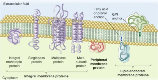
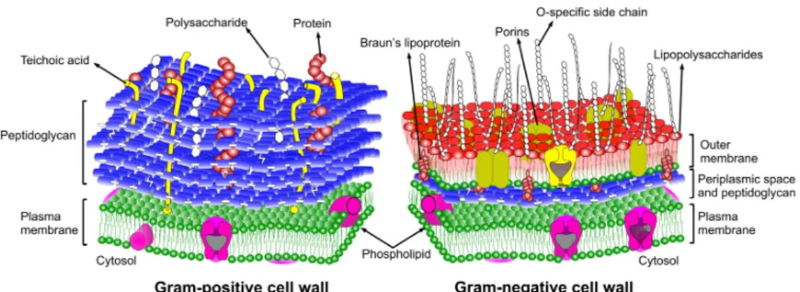
(37) Thèse de Antoine Dujardin, Université de Lille, 2018. 2. Atomic Force Microscopy. 2.3.2. Sample Preparation While able to work in biological conditions, one of the main drawbacks of AFM is that microscopic samples have to be immobilized on surfaces for scanning. In particular, the immobilization needs to withstand shear forces as the cantilever is scanned over the sample. Cells are presented in Section 3.1. Unless spontaneous, their immobilization can usually be achieved by chemical binding or physical confinement. Eukaryotic Cells Epithelial cells, such as the ones described in Section 3.2.4, simply have to be seeded and adhere easily. Their very soft nature allows them to have a good contact area with the substrate. Some other kind of cells are more difficult to immobilize but are not the focus of this project. Yeast cells, such as Saccharomyces cerevisiae, do not spontaneously adhere but can be immobilized mechanically in porous membranes (Kasas and Ikai, 1995) or embedded in an agar matrix (Gad and Ikai, 1995). A hybrid chemical and physical immobilization method was also developed with microstructured, concanavalin A-functionalized PDMS stamps (Dague et al., 2011). Prokaryotic Cells Prokaryotic cells are difficult to immobilize, as their structure is more rigid than most eukaryotic cells, limiting the surface available for adhering with the substrate (Dufrêne, 2004). In most cases, the cells do not adhere naturally to the glass support enough to resist the forces applied by the cantilever, although very small, or stay stable during the scan. One way to immobilize bacteria is to dry and rehydrate them, as the drying forces the interactions between the cell and the substrate. Although being one of the simplest—hence frequently used—method, it is one of the most damaging for the cell integrity. It leads to the decrease of their height. 26. © 2018 Tous droits réservés.. lilliad.univ-lille.fr.

(38) Thèse de Antoine Dujardin, Université de Lille, 2018. 2. Atomic Force Microscopy. and width combined with the appearance of patterns at the surface, indicating a strong impact of the immobilization on their viability (Bolshakova et al., 2001). This strong impact can be useful to image topographical elements that would be otherwise invisible because too soft and motile, such as some flagella and pili, but it is necessary to keep in mind that the properties of the cell have been altered strongly (Gillis, Dupres, Delestrait, et al., 2012). Drying is therefore to be avoided and cell immobilization has to be artificially mediated, chemically or physically. Chemical binding includes covalent binding. It can, for example, be performed by coating the substrate with 3-aminopropyltriethoxysilane (APTES). Its three ethoxy groups react with the hydroxyl groups from the glass surface to form a covalent oxygen bond between its silicon and the one of the glass. The APTES then becomes the surface of the glass, exposing its amine group. Crosslinkers, such as glutaraldehyde, can then be used to connect the amine groups of the substrate with the ones of the sample (Karrasch et al., 1993). Crosslinking should be avoided, however, as it changes the mechanical properties such as the stiffness and adhesion of the sample (Burks et al., 2003). Non-covalent binding can be caused by poly-l-lysine (PLL) (Karrasch et al., 1993) or polyethylenimine (PEI) (Razatos et al., 1998), in which the adhesion is induced by charge differences between the cell surface and the substrate. Gelatin is another option, believed to act from a mix of hydrophobicity and the effect above (Doktycz et al., 2003). Adhesive proteins, such as Cell-Tak™ (BD Diagnostics), poly-dopamine, cyanoacrylate, and lectins such as concanavalin A, can be used as well (Louise Meyer et al., 2010; Ozkan et al., 2018). Porous membranes, mentioned earlier for yeast cells, can also be used in bacteria, especially spherical ones (van der Mei et al., 2000). It should be noted that this technique could have been interesting to host our prokaryotic samples, rather than the glass coverslip introduced in Chapter 6. It has, however, its own limitation as it limits the accessible area to the emerging part of the cell. It also complicates the sample topography, hence the. 27. © 2018 Tous droits réservés.. lilliad.univ-lille.fr.

(39) Thèse de Antoine Dujardin, Université de Lille, 2018. 2. Atomic Force Microscopy. detection procedure required to localize the bacteria. No unique method works universally for all kinds of cells. Different methods perform differently depending on the cell type, the required medium (concentration of biological matter, composition, pH. . . ), and the system requirements (such as a transparent support when using an inverted microscope) (Louise Meyer et al., 2010).. 2.4. PeakForce Given the shear forces of contact mode, the low force control of tapping mode, and the slowness of force volume, a mode avoiding their caveats was much needed. PeakForce Tapping, which performs super-fast pseudo force curves, presents the advantage of the force control of force volume, but with a speed much closer to the one of imaging modes. Although technically an AFM mode, it is treated here separately as it is of particular importance for this work. It shares a lot of similarities with several of the other modes while being much more complex. The documentation around it is scarce or vague and its functioning tends to be poorly understood. For these reasons, it is often used with too much optimism and blind trust in its results or, oppositely, unduly criticized.. 2.4.1. Off-Resonance Tapping PeakForce is part of the off-resonance modes, which share similarities with tapping mode in that they avoid shear forces by only having an intermittent contact with the sample. Here again, the vertical position of the tip in time forms a sinusoid. Off-resonance modes are, however, different in that they operate much below the resonant frequency of the cantilever, usually by at least an order of magnitude. This strongly limits the amplification effect, so that the amplitude at the end of the cantilever is the same as the one applied by the piezo and the deflection stays constant (null) in the absence of interaction with the sample or the medium, as an opposition to. 28. © 2018 Tous droits réservés.. lilliad.univ-lille.fr.

(40) Thèse de Antoine Dujardin, Université de Lille, 2018. 2. Atomic Force Microscopy. oscillating modes where the cantilever would actually oscillate, creating an oscillation in the deflection. As a consequence, the sinusoidal movement of the tip is due to the oscillation of the cantilever in tapping whereas it is solely due to the oscillation of the piezo in PeakForcce.. 2.4.2. Pseudo Force Curves Given that the cantilever stays straight in the absence of force, the approachretract movement of the tip is actually more similar to a force curve. The major difference with conventional force curves is that they have an approach at a constant speed, then a sudden reverting of the movement at the trigger point, and a retraction at a—possibly different—constant speed, whereas the oscillation-like movement of PeakForce gives it a smooth transition. A normal force curve and its PeakForce equivalent are shown in Figure 2.10. Compared to their straight equivalent, one can note from Figure 2.10 that the PeakForce curve is much smoother. The smoothness in C compared to 3 in the left two images is due to the progressive deceleration and opposite acceleration of the piezo when moving from the approach to the retract sections in contact with the sample. This smoothness disappears when the time axis is changed to the piezo position one, giving back the linear end of a force curve in the corresponding graphs on the right. A second difference is the smoothness of points B and D compared to their 2 and 5 equivalents. The non-contact part, especially, is supposed to be vertical, as it can be seen in the top graphs. The reason for this smoothness is the proximity of the resonant frequency of the cantilever, which limits the speed of the tip relative to the piezo. In the case of the force curves, the movement appears vertical because of its low speed, but similar effects would be observed should the force curve be taken at the same speed. Similarly, the effect does not appear in PeakForce when stiff cantilevers are used. Another important difference is that, whereas force curves retract when. 29. © 2018 Tous droits réservés.. lilliad.univ-lille.fr.

(41) Thèse de Antoine Dujardin, Université de Lille, 2018. 2. Atomic Force Microscopy. Figure 2.10.: Comparison scheme between force curves and their PeakForce equivalent. Top: force curve. Bottom: PeakForce. Left: deflection as a function of time. Right: deflection as a function of the vertical position of the piezo, for the approach (blue) and retract (red). 1/A: non-contact approach. 2/B: snap-in contact. 3/C: trigger force/peak force. 4: 0-force contact. 5/D: maximum adhesion force (snap-off contact). 6/E: noncontact retraction. © Bruker, modified.. 30. © 2018 Tous droits réservés.. lilliad.univ-lille.fr.

(42) Thèse de Antoine Dujardin, Université de Lille, 2018. 2. Atomic Force Microscopy. triggered by the force threshold, the vertical movement of PeakForce curves is set at the beginning of the curve. Rather than retracting on a threshold, a feedback loop is applied on the detected peak force from one curve to another.. 2.4.3. Operation PeakForce can be used mainly in two circumstances: as a simple imaging mode or to extract nanomechanical information by analyzing the pseudo force curves. It operates at a set of given frequencies. Common values are 0.125 kHz, 0.25 kHz, 0.5 kHz, 1 kHz, 2 kHz, and 8 kHz and should be selected carefully. Since the feedback is based on the previous curves, a higher frequency allows a faster feedback, hence a better tracking of the surface at high speed. It also limits the horizontal distance per cycle, therefore reducing shear stress. On the other hand, operating at high frequency causes increased hydrodynamic effects when operating in fluid. When approaching one tenth of the resonant frequency of the cantilever, ringing effects can also be noticeable, deteriorating the quality of the force curve. As a consequence, the technique can be used at high frequencies when focused on imaging but lower frequencies should be preferred when the quality of the curves is of importance (i.e. when probing nanomechanical properties), although the optimal values depend on the cantilever and the medium. To work on soft samples, however, soft cantilevers have to be used. As discussed in Section 2.1.1, on most traditional cantilever designs, the resonant frequency goes in par with the spring constant. This made PeakForce initially difficult to use on soft samples, until the development of new cantilever designs, allowing a low spring constant with a comparatively high resonant frequency (Schillers, Medalsy, et al., 2016).. 31. © 2018 Tous droits réservés.. lilliad.univ-lille.fr.

(43) Thèse de Antoine Dujardin, Université de Lille, 2018. 2. Atomic Force Microscopy. 2.4.4. Hydrodynamic Effects In liquid, the hydrodynamic effect applies to the cantilever a force opposite to its movement. While this effect is not specific to PeakForce since it would also apply to any movement at similar speeds, it is less common to reach these speeds with other modes. Furthermore, specific algorithm are applied in this situation. During the sinusoidal movement, the speed of the cantilever is most important in the middle of the approach and retract curves and much lower when it touches the sample. Thus, the hydrodynamic effect mostly affects the non-contact parts of the curves, inducing what appears to be a repulsive force during the approach and an attractive one on the retraction. This background effect mostly resembles a sinusoid, although its phase is delayed by a quarter of the period. A first method to cancel the background effect consists of recording PeakForce curves slightly above the sample, hence without close-range tipsample interactions. This background data is then subtracted from further force curves. Whereas this method can be sufficient on most materials, the hydrodynamic effect is especially critical on cells, where the softness and large topographical features impose a large PeakForce Amplitude (600 nm peak to peak), causing at high speed hydrodynamic forces that can reach 20 nN on most standard cantilevers geometries, more than a higher of magnitude higher than the typical setpoint (Schillers, Medalsy, et al., 2016). Furthermore, the height of the cells can sometimes be close to the total height of the tip—or, at least, non-negligible. This brings the distance between the sample and the cantilever (not the tip) significantly smaller when the tip is scanning a lower part of the cell while the nucleus is under the cantilever. Oppositely, the cantilever-sample distance is significantly bigger than its normal value when the tip is scanning the top of the cell while the cantilever is over an empty area. This creates variations in the hydrodynamic background, lowering the efficacy of the method described above.. 32. © 2018 Tous droits réservés.. lilliad.univ-lille.fr.