A sharp immersed boundary method based on penalization and its application to moving boundaries and turbulent rotating flows

Science Arts & Métiers (SAM)

is an open access repository that collects the work of Arts et Métiers Institute of

Technology researchers and makes it freely available over the web where possible.

This is an author-deposited version published in: https://sam.ensam.eu

Handle ID: .http://hdl.handle.net/10985/17886

To cite this version :

Mathieu SPECKLIN, Y. DELAURÉ - A sharp immersed boundary method based on penalization

and its application to moving boundaries and turbulent rotating flows - European Journal of

Mechanics - B/Fluids - Vol. 70, p.130-147 - 2018

Any correspondence concerning this service should be sent to the repository

Administrator : archiveouverte@ensam.eu

A sharp immersed boundary method based on penalization and its

application to moving boundaries and turbulent rotating flows

M. Specklin

a,b,

_{*, Y. Delauré}

a

a_{School of Mechanical and Manufacturing Engineering, Dublin City University, Glasnevin, Dublin, Ireland} b_{Sulzer Pump Solutions Ireland Ltd., Wexford, Ireland}

a b s t r a c t

This paper presents an Immersed Boundary Method (IBM) for handling flows in the presence of fixed and moving solids with complex geometries. The method is based on a penalization approach and designed to preserve the sharpness of the immersed boundaries. Corrections of the boundary conditions are implemented at the interface to improve the accuracy of the solution in comparison to first-order methods and avoid the rasterization issue on Cartesian grids.

The current IBM is developed in the OpenFOAM⃝R _{library (-v 2.2) and its accuracy is first verified}

against the Wannier flow case. It is then applied to the flow in presence of fixed and moving circular obstacles. The computational results show good agreement with equivalent standard body-conforming simulations and other high order published IBM, and demonstrate as well that improvements can be achieved by correcting the boundary conditions for both velocity and pressure on the interface. Finally, the method is assessed by reference to a realistic engineering application involving rotating flow: a single-phase mixer. In this case, the method is coupled to a DES model for turbulence modeling, and results show again good comparison with experimental results.

1. Introduction

Although the accuracy of CFD methods handling complex mov-ing geometries has increased in recent years, with new high order sliding mesh methods [1–3] for instance, or Arbitrary Lagrangian– Eulerian (ALE) techniques for Fluid–Structure-Interaction (FSI) [4–8], meshing complex realistic engineering systems remains a significant challenge in a wide range of applications. The additional mesh constraints imposed by sliding interfaces can make it espe-cially difficult to achieve good quality refined mesh in particular in compact designs where thin gaps between moving boundaries are not uncommon. Immersed Boundary Methods (IBMs) have shown to be good alternatives for a broad range of problems. Their aim is to solve a single set of conservation equations for several physical components that can be gas, liquids or more commonly solids, without the need for a mesh which conform to the inter-phase boundaries. As a result, IBMs make it possible to handle multi-phase flow problems and fluid–structure interaction problems, both in a single-phase framework. One of the main interests of IBM lies thus in the simplification of the model. Of particular impor-tance is the method’s suitability for use with simple Cartesian grids

*

Corresponding author at: School of Mechanical and Manufacturing Engineer-ing, Dublin City University, Glasnevin, Dublin, Ireland.

E-mail address:mathieu@specklin.ne(M. Specklin).

which can guarantee second order accuracy and improve stability of the numerical solution. This strongly reduces the time required to setup the computational case, which can be significant with complex and moving geometries. Special care must then be taken to obtain the correct boundary conditions at the exact position of the interface, and to reproduce the effects of the real geometry. The imposition of the boundary condition is a key point of the methods and it is also what differentiate IBMs from each others.

The first documented IBM was implemented by Peskin [9] to model the interaction of the blood flow with an heart valve, mod-eled as non-conforming elastic solid. For this method, the effect of the solid is smeared on the cells in the vicinity of the inter-face, by introducing a fictitious force in the momentum equation, combined with a well chosen discretized Dirac delta function. The forcing term and solid velocity are calculated from constitutive law, as the Hook’s law if the immersed surface exhibits elastic de-formation. Approaches of this type are named continuous forcing approach, as the Immersed Boundary (IB) force is added before the discretization of the equations. Extensions of this kind of methods have been proposed to deal with solid boundaries in the rigid limit. In this case, the forcing term can be modeled for example as a spring restoring force (see work of Lai and Peskin [10]), or can be obtained in a feedback way thanks to an already known solid velocity as proposed by Goldstein et al. [11]. However, these approaches are subject to stiffness problems in the limit of rigid

solids, due to the high gradients of the forcing term. The Dirac delta function, used to map the variables from the fluid Cartesian grid to the solid Lagrangian grid, has the effect of blurring the location of the solid interface. High spatial resolution is thus required in order to retrieve a sharp representation of the interface.

In the same spirit of the method of Goldstein et al., the approach of Angot et al. [12] uses a forcing term based on the Brinkman equation for porous media, to obtain the desired no-slip velocity at the solid interface. This type of method belongs to the class of penalization methods, and has been widely used for immersed boundary problems, even with complex geometries as in fish-like swimming applications ([13,14] and [15]). However, most of published methods do not reach second order accuracy in space. To the author’s knowledge, the Sub-Mesh Penalty Method of Sarthou et al. [16], the second order Penalty model of Introïni et al. [17], and the work of Chantalat et al. [18] are the only models based on penalization which offer improvements to tackle the rasterization effect on Cartesian grids. In addition, the active zone for the forc-ing term is generally also diffused by the use of mask functions combined with Heaviside functions, as it is the case in [19] and in [14]. A different type of penalization method has been proposed by Vincent et al. [20], where the stress tensor is penalized instead of the velocity, and has been applied to particle-laden flows. Concern-ing the application areas, penalization methods have been used for compressible flows ([21] and [22]), combined with level-set methods for interface tracking problems ([13,18] and [14]), used for fluid–structure interactions problems as in [23] or [24], or again used for highly turbulent flows ([13] and [25]).

The IBM presented in this article is based on a penalization approach as well, and is implemented in the Open Source solver library OpenFOAM⃝R

. Two penalization methods have already been implemented on this platform. Firstly, in order to study wettability conditions, the first order model of Horgue et al. [26] was com-bined to the Volume-Of-Fluid method. Secondly, Blais et al. [27] combined the pressure implicit with splitting of operators (PISO) scheme of OpenFOAM⃝R

with an IBM formulation based on vol-ume correction. Although with a similar level of error, the lat-ter method degrades the order from 2 to 1.33 in comparison to the standard PISO scheme on body-fitted mesh. Our penalization technique proposes to address both weaknesses of diffusion and low order of accuracy. The forcing term employed in the model is active strictly only inside the immersed solid, and does not use smearing functions. This feature allows a sharp representation of the geometry and its interface. In order to enhance the order of accuracy, the velocity is corrected inside the solid and in the vicinity of the interface, with a linear interpolation. Furthermore, the pressure is penalized on the same cells in order to avoid a spurious contribution to the pressure gradient in the momentum predictor and to the solution of the pressure equation.

In Section2, the formulation of the present penalization ap-proach is developed, including the corrections implemented for the velocity and the pressure near the interface. Particular attention is paid to (i) the estimation of the force exerted by the fluid on the solid, used for the calculation of the drag for instance, and (ii) the combination of the IBM with a DES turbulence model (DES– IBM), involving a specific treatment for the turbulent viscosity. The accuracy of the model is assessed by reference to the Wannier case, which is presented in Section3, along with three other test cases involving moving and complex boundaries in laminar and turbulent rotating flows. For the turbulent case, a power-law based method for correcting the velocity at the immersed surface is introduced. This approach complies with the velocity profile of an attached boundary layer. The sensitivity of the results to the two types of velocity reconstruction is then discussed. The efficiency of the present IBM is demonstrated and compared to equivalent body-fitted mesh simulations. Finally, Section4summarizes and concludes the current formulation.

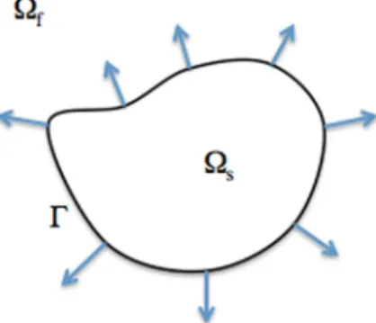
Fig. 1. Sketch of the different domains.

2. Numerical formulation

2.1. Immersed boundary formulation

Consider a rigid solid represented byΩs, immersed in a fluid domainΩf, as illustrated inFig. 1.Γis the interface between both domains. In the IBM presented in this study, the Navier–Stokes equations are solved in the entire domainΩ

=

Ω_f

∪

Ω_s.

2.1.1. Treatment of the solid geometry

The interface of the immersed solid Γ is represented by a discrete mesh which may be made of triangular or other polyhedral faces. The mesh is characterized by a set of Lagrangian points xib,n, with n from 0 to N, N being the number of solid points. These points represent the face centers of the surface mesh. The latter is used to identify the cell centers inside the solid domain from those inside the fluid domain, thanks to an octree partition of space.

2.1.2. Governing equations

An isothermal and incompressible flow is governed by the following equations of mass and momentum conservation:

∇ ·

u

=

0 (1)

∂

u

∂

t

+ ∇ ·

(uu)

−

ν∇

2_u

₊

_f

_{= −∇}

_{p (2)}

where u is the velocity, p the pressure,

ν

the kinematic viscosity and t the time. In Eq. (2), f is the forcing term, or immersed boundary force, which is required to impose the correct bound-ary condition for the velocity at the interface with the immersed solid. This force is here strictly only active inside the solid, and its formulation is discussed below.

2.1.3. Penalization of the velocity

The immersed boundary method presented in this paper is based on the Penalty method, first introduced by Arquis [28]. In this approach, the immersed solid is considered as a porous media, with a very small permeability 0

<

K

≪

1. Hence the forcing term of Eq.(2)can be written in the following form:

f

=

χ

ν

K(u

−

uib) (3)

where uibis the velocity of the Immersed Boundary (IB) and

χ

is a characteristic function, which makes possible the localization of the solid. This function is defined in the equation below:

χ

(x

,

t)

=

{

1 if x

∈

Ω_s(t)

0 if x

∈

Ωf(t)

.

(4)

The forcing term is then not enabled in the fluid domain, and the original momentum equation is thus obtained. Angot et al. have

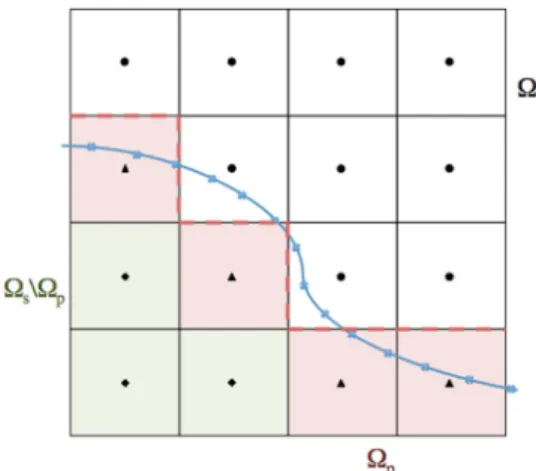
Fig. 2. Sketch of the discrete domains. The discrete solid domain is delimited by the

dashed red line.•are the cell centers in the fluid domainΩf. ♦ are the cell centers in

the solid domain, except the penalized domain,Ωs\Ωp, in green, and ▲ are the cell

centers in the penalized domain in red.×are the solid points (in blue). The grids considered in this study are made of cubic cells and uses the collocated storage of OpenFOAM⃝R_.

Fig. 3. Sketch of the velocity correction scheme on a 2D Cartesian mesh. The same

nomenclature is used for the domains definition.

shown in [12] that this formulation is equivalent to the standard incompressible Navier–Stokes equations with a Dirichlet condition at the interfaceΓfor the velocity, and the authors have presented rigorous estimation of the errors introduced by this formulation as well as convergence theorems. In the cases considered in this doc-ument, the velocity of the immersed body uibin Eq.(3)is always a geometrical velocity which is known and time-dependent. 2.1.4. Correction scheme for the velocity near the interface

For Cartesian grids, the forcing term presented in Eq.(3)leads to a stair-case definition of the solid geometry as shown inFig. 2. Furthermore the cell centers, where the solid velocity is imposed, do not necessarily coincide with the solids points representing the immersed body. Two main errors are introduced with a simple Penalty approach. Firstly, the interface orientation is not accounted for, and secondly, the Dirichlet condition is not necessarily satisfied at the exact position of the interface.

In order to address these issues, Chantalat et al. [18] have proposed for elliptic problems an iterative correction of the nor-mal derivative of the solution at the interface. A more intuitive approach is to impose a corrected velocity in the cells near the

interface, chosen to ensure that the Dirichlet condition u

=

uib is satisfied at the exact interface position. Practically, this means that the corrected velocity is a function of both the solid velocity and the fluid velocity in the close neighboring area. In the Sub-Mesh Penalty Method of Sarthou et al. [16], this corrected ve-locity is obtained by linear interpolation between the solid and the fluid velocities. In [17] the corrected velocity is evaluated from an averaged reconstruction of the velocity gradient for the fluid contribution, and by means of a minimization problem for the solid contribution. The IB force is then scaled with the solid characteristic function or the cell volume ratio, and the modified Navier–Stokes equations are solved with a fractional-step method, which takes into account the forcing term in the correction step as well, as suggested by [29] for a consistent imposition of the boundary condition at the interface.

Similarly to the work of Sarthou et al., the correction scheme considered here is based on an interpolation of the velocity im-posed in the vicinity of the fluid–solid interface. In this context, the forcing term introduced in Eq.(3)is re-defined as:

f∗

=

χ

ν

K(u

−

uib)

+

χ

∗

ν

K(u

−

u ∗ p) (5) where

χ

∗

stands for the characteristic function which represents an internal layer of cells, and where the modified velocity is applied

u∗

p. The new characteristic function defines a domainΩp, in red in

Fig. 2, named here as the penalized domain and used in Eq.(6):

χ

∗

(x

,

t)

=

{

1 if x

∈

Ω_p(t)

0 else

.

(6)

More precisely, each cell inΩspossessing at least one neighbor in

Ωfis included inΩp. In addition, the support of the characteristic function introduced in Eq.(4)for the imposition of non-modified solid velocity is changed fromΩstoΩs

\

Ωp. It is important to note that the momentum forcing is enabled everywhere inside the solid domain, either to impose the interpolated velocity or the solid velocity. Thereby, the implementation of the correction scheme for the velocity does not introduce a reversed fictitious velocity inside the IB, as it is the case for IBMs in which the unmodified Navier– Stokes equations are solved inside the IB [30]. The imposed velocity

u∗

pin a cell ofΩpis calculated from a linear extrapolation, using the closest solid point of the interface and a virtual point in the fluid domain on the normal direction, as described in Eq.(7):

u∗_p

=

d1

+

d2 d2 uib,n

−

d1 d2 u_φ

=

d1

+

d2 d2 uib,n

−

d1 d2 (

∑

k

α

kuq,k

+

β

uq)

.

(7)

In the above equation, d1 and d2 represent respectively the approximate distance from the cell center P to the interface, and the distance from the interface to a virtual point

φ

, along the interface normal. The procedure is illustrated inFig. 3. Similar correction schemes have been employed for instance in the IBM of Tseng and Ferziger [31] and in the Penalty method of Sarthou et al. [16]. Two types of case studies will be discussed in the present manuscript. The first considers academic problems involving im-mersed geometries which can be defined analytically. In this case the distance to the interface can be determined exactly and the Dirichlet condition u

=

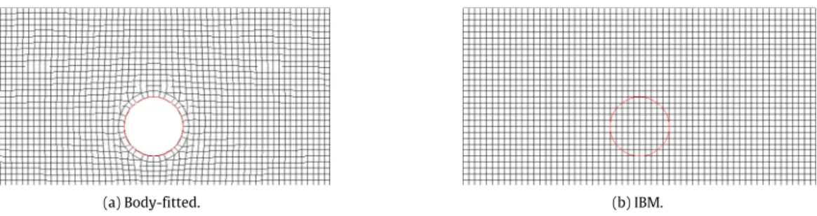
uib,nis thus satisfied at the exact interface position. The second considers more realistic engineering systems with relatively complex immersed boundaries. In which case de-termining the exact interface position is not possible. Two options have been considered: estimate the position (i) with a dichotomy algorithm or (ii) simply using the closest solid point xib,n. The former iterative approach can converge reasonably quickly but the increase in the computational is not negligible with high surface refinement. The error introduced in this case can be significantly

(a) Body-fitted. (b) IBM.

Fig. 4. Sketch of the grids used for the 2D Wannier test case, with 10 cells in the cylinder diameter for the IBM, and the equivalent body-conforming mesh. The surface mesh

of the cylinder is represented in red. (For interpretation of the references to color in this figure legend, the reader is referred to the web version of this article.)

reduced with a sufficient refinement of the solid surface mesh, and was found negligible in the test cases considered in this work. This result is discussed in Section3.4.2. It is important to note however that this discrepancy may prevent the model of achieving a formal second order accuracy in realistic application. Regarding the accuracy of the solution as a function of the parameters d1and d2, it was verified for the Wannier case (presented in Section3.1) that d2

=

d1 gives the best results. Finally, the velocity at the virtual point u_φ is also obtained thanks to a linear interpolation of the velocity at the center of the cell Q , holding the virtual point, and velocities at different points k on the closest face of the considered cell. Thereby,

α

and

β

in Eq.(7)are the coefficients of the linear combination. The velocities at the face corners ui,kare again estimated through interpolation from the neighboring cells.

2.1.5. Estimation of the immersed boundary force

The physical force F exerted by the fluid on the solid can be decomposed into pressure and viscous terms:

F

= −

∫ ∫

Γ pdS

+

µ

∫ ∫

Γ (T

·

n)dS (8)

where dS is a small element of surface on the immersed boundary interfaceΓ, and n and T represent respectively the normal at the solid interface and the strain rate tensor. The estimation of this force requires additional and delicate computations. Indeed, as the surface of the immersed body does not necessarily coincide with the faces of the Eulerian grid, a reconstruction of the variables at the Lagrangian solid points is usually implemented [32,33]. In the present study, a different approach is adopted, which is based on the Gauss’s theorem. Applying the latter to a domain_Ω

˜

surrounding the immersed body allows to rewrite Eq.(8)as:

F

= −

∫ ∫ ∫

˜ Ω

∇

pd_Ω

˜

+

∫ ∫

˜ Γ pdS

+

µ

∫ ∫ ∫

˜ Ω

∇

2ud_Ω

˜

−

µ

∫ ∫

˜ Γ (T

·

n)dS (9)

whereΓ

˜

represents the boundaries of the domainΩ

˜

, excluding the immersed interfaceΓ. With a relevant choice of_Ω

˜

_{, Eq.(9)}

can be discretized easily, in accordance with the considered mesh, in order to estimate the force applied by the fluid. Furthermore, the volume integral terms can also be replaced by the transient and convective terms thanks to the Navier–Stokes equations, as described in Eq.(10): F

=

ρ

∫ ∫ ∫

˜ Ω

∂

u

∂

td

˜

Ω

+

∫ ∫

˜ Γ pdS

+

ρ

∫ ∫ ∫

˜ Ω

∇ ·

(uu)d_Ω

˜

₋

_µ

∫ ∫

˜ Γ (T

·

n)dS

.

(10)

2.2. Discretization techniques and solution solver

The discretization procedure for the Navier–Stokes equations are based on the work of Jasak [34], following a Finite Volume formulation. All the variables are stored at the cell centers, where a non-staggered grid arrangement is used. The procedure of Jasak uses a predictor–corrector algorithm for the pressure–velocity coupling (PISO scheme), whose formulation is detailed below with combination to a pressure correction accounting for the immersed boundary presence. The equation are discretized in time with an Euler implicit scheme, and using second order schemes in space. 2.2.1. Momentum predictor

The first step of the method consists in estimating an inter-mediate velocity field, thanks to a semi-discretized momentum equation:

aiu

˜

i

=

H(u)

˜

− ∇

pn

.

(11)

The predictor for the velocity is calculated from the pressure at the previous known time step n. In the matrix system (11),u

˜

i represents the numerical estimation of the intermediate velocity at the center of the ith cell, and aiis the diagonal matrix coefficient for the cell i. The term H(u), includes the contribution from neigh-

˜

boring cells, the explicit part of the transient term, and all other source terms. The forcing term f introduced in Eq.(2)includes an implicit contribution, involving the fluid velocity, and an explicit contribution, involving the solid or corrected velocity. The implicit part thus modifies directly the diagonal matrix coefficients ai, while the explicit part is included in the term H(u). This term finally

˜

reads for a cell inside the solid domain:

H(u)

˜

= −

∑

j aju

˜

j

+

un i ∆t

−

uib K

.

(12)

If one considers a cell inside the domainΩp, the solid velocity uib is replaced by the corrected velocity u∗

pin Eq.(12). In the latter, j stands for the neighboring cells, n represents the previous iteration time step and∆t is the value of the time step. The contribution of the neighboring cells for the term H(u) is obtained by a lin-

˜

earization of the quadratic convection term, which implies that a flux satisfying the mass conservation equation at time n is used to calculate the matrix coefficients aiand aj.

2.2.2. Pressure solution and PISO loop

The second step of the discretization procedure is to solve the pressure equation. This equation is derived from the momentum equation(11), by imposing mass conservation (

∇ ·

u

=

0). Gradient and divergence terms are discretized using the Gauss theorem, providing an equation for pressure:

∑

f Sf

· [

( 1 ai )f(

∇

pm)f

] =

∑

f Sf

·

( H(um₎ ai )f (13)

where Sfis the outward normal surface vector for the face f of the ith cell. The resulting matrix for pressure is solved with an iterative method. One can note that the pressure does not depends directly on the intermediate velocity field, but only on its contribution through the term H(um). Here, m stands for the increment of the PISO loop, whose initial conditions are given by um

₌

_{u and}

_˜

pm

₌

_pn_{at the initial iteration m}

₌

_0.

The new face flux and cell center velocity are calculated from the new pressure field. Eq.(14)gives the new conservative fluxes, which will be used to build the matrix system for the momentum predictor at the next time step. The velocity is corrected explicitly with Eq.(15). The value at the faces are obtained using interpola-tion techniques. Fm+1

=

Sf

·

um +1 f

=

Sf

· [

( H(um₎ ai )f

−

( 1 ai )f(

∇

pm)f

]

(14) um_i+1

=

⎧

⎪

⎨

⎪

⎩

H(um₎ ai if i

∈

Ω_s

∪

Ω_p H(um₎ ai

−

1 ai

∇

pm else

.

(15)

The velocity correction step, defined by Eq. (15)to account for the corrected pressure field, is modified in the solid and the penalized domains. As the intermediate velocity estimated from the momentum predictor step does satisfy the boundary condition determined by the momentum forcing, this velocity correction step is not necessary in the latter domains. Because the velocity correction step is explicit, several iterations of pressure solutions and explicit velocity corrections are necessary (usually two or three) to take into account the transported influence of the correc-tions of neighboring velocities. After solving the velocity correction step for um+1_{, the term H(u}m_{) is recalculated and a new increment} is performed as m

→

m

+

1. Once a predetermined convergence criterion is achieved, velocity and pressure are updated for the next time step with un+1

₌

_um+1_{and p}n+1

₌

_pm_.

Finally, it is worth noting that the Rhie–Chow discretization procedure is adopted to avoid checker-boarding on the collocated grid [35]. The cell face fluxes are interpolated from the momentum equation (Eq.(14)) and then used to derive the pressure correction equation (Eq.(13)) from the continuity equation.

2.2.3. Boundary condition for pressure at the immersed interface For continuous IBM with diffuse interface, no pressure bound-ary condition is usually needed on the immersed boundbound-ary [36], as the influence of the solid is smeared over several layers of cells. In the current sharp interface method however, the effect of the solid interface on local mass conservation must be taken into account in the solution of Eq.(13), for the pressure to be correct at the IB. The error introduced by a non-conservation of mass locally is furthermore accentuated by the mirrored velocities obtained from interpolation (see Section2.1.4) and generates an un-physical pressure field near the IB. This issue has been considered in details by Kang et al. [37] for a discrete IBM, where a decoupling constraint for the pressure is proposed, and combined with a compatible interpolated velocity boundary condition related to mass conser-vation. Kim et al. [38] developed a method introducing a mass source/sink in addition to the momentum forcing, in order to sat-isfy the continuity in the cells containing the immersed boundary. In the current approach, the pressure is corrected directly at the interface so that the local mass conservation error does not propagate into the fluid domain from the solid domain. Without correction, the spurious pressure in the domainΩpmay influence the pressure solution in the neighboring fluid cells. Indeed in those fluid cells, both the evaluation of the pressure gradient in the momentum predictor and the discretization of the Laplacian term in the pressure solution step, involve the pressure inΩp. As

OpenFOAM⃝R

uses a small computational molecule, strictly only the cells inside the latter domain can influence the pressure in the fluid. Therefore, a correction of the pressure computed during the pressure equation step is adopted in the penalized domain. Namely, for a cell P ofΩp the lower and upper triangles of the matrix build from Eq.(13), representing the contribution from neighboring cells, are canceled, while the source term is modified in order for the pressure to be imposed at the desired value. The latter value is chosen to be equal to the pressure at a virtual point along the interface normal n, in accordance to a Neumann boundary condition (_∂∂_np

|

_Γ

=

0). The pressure at the virtual point p_φ is obtained by linear interpolation, similarly to the velocity corrections introduced earlier:

pp

=

pφ

=

∑

k

α

kpk

+

β

pq

.

(16)

2.3. Turbulence modeling

From an engineering point of view, a RANS model for turbulence can be sufficient to give good estimation of general integrated quantity. However, in order to capture the turbulent features of the flow, which can have a significant effect on the transport of a secondary phase in a multiphase flow, it is necessary to consider scale resolving simulation using for example Large Eddy Simula-tion (LES) models. The IBM presented here has been extended to include a hybrid RANS–LES turbulence model. A Detached-Eddy Simulation (DES) model [39] was coupled to the current penal-ization approach, taking advantage of the RANS modeling for the wall layer, while using a LES outside of this region to resolve all the scales of turbulence up to the filter size. The relative simplicity and robustness of the Spalart–Allmaras (SA) model makes it a good candidate for the RANS approach. In addition, the similarities of modeling between the SA model and a standard LES formulation for the turbulent viscosity simplifies the coupling of the RANS and LES models. The combinations of our IBM with the SA and the DES models are respectively discussed in Sections2.3.1and2.3.2. 2.3.1. IBM formulation of the Spalart–Allmaras model

The standard Spalart–Allmaras model assumes a zero Dirichlet condition on a wall surface for the turbulent viscosity

ν

t [40]. In order to satisfy this boundary condition on the immersed bound-ary, the standard SA model has been modified to take into account the presence of the immersed body, using a penalization method similarly to the momentum equation. The Dirichlet condition is thus imposed for the turbulent viscosity inside the whole solid. Furthermore, for a better representation of the immersed interface, a corrected viscosity is imposed in its vicinity, similarly again to the correction scheme of the velocity.

In OpenFOAM⃝R

, the SA model requires the solution of the transport equation for a modified kinetic viscosity

ν

˜

. The turbulent viscosity is obtained from the latter according to:

ν

t

= ˜

ν

fv1 (17) where:

⎧

⎨

⎩

f_v1

=

χ

3

χ

3

₊

_c3 v1

χ = ˜ν/ν.

(18)

The penalized version of the transport equation for the modified turbulent viscosity finally reads:

D

ν

˜

Dt

=

P

−

D

+

1

σ

(

∇ ·

(

ν + ˜ν

)(

∇ ˜

ν

)

+

cb2(

∇ ˜

ν

)2)

+

χ

Kν˜ (

ν − ν

˜

_ib)

+

χ

∗ Kν˜ (

ν − ν

˜

_p∗)

.

(19)

In Eqs.(18)and(19), P and D stands for the production and de-struction terms which are implemented as defined by Spalart and Allmaras in [41], while c_v1and cb2are constants of this model, and finally

σ

is the turbulent Prandtl number. Regarding the imposition of the boundary condition,

ν

ibstands for the zero immersed body viscosity, while

ν

∗

pis the corrected viscosity taking into account the position and the orientation of the interface. As for the penalization of the velocity,

χ

,

χ

∗

and K_νtdenotes here the characteristic

func-tions and the penalization coefficient associated to the turbulent viscosity. Finally cb1and cb2are constants of the standard SA model, while

σ

is the turbulent Prandtl number. The corrected viscosity

ν

∗

p is estimated by an interpolation between

ν

ibat the position of the interface and the value of the turbulent viscosity in the neighboring fluid area, similarly to the algorithm used for the penalized velocity in Eq.(7). A similar type of correction has been used by Balaras in [42].

2.3.2. IBM–DES

In the DES model, the transition from RANS to LES is triggered by the following parameter:

˜

d

=

min(d_w

,

CDES∆)

.

(20)

In Eq.(20), d_w stands for the distance to the wall, CDES is a con-stant usually set to 1 and ∆defines the grid spacing as ∆

=

(∆x∆y∆z)1/3. When d_w

≤

∆the models acts as the SA model, while for∆

≤

d_wit acts as a LES model.

The IBM of this work is then combined with the DES model by merely changing d_wto d∗

was detailed in Eq.(21).

d∗_w

=

min(d_w

, ψ

) (21)

where

ψ

is the distance function to the immersed boundary. There-fore, the model is acting as well as a SA model in the regions near the walls of the immersed solid.

3. Results and discussions

The current IBM has been validated against several test cases, covering different types of geometries for the solid and flow reg imes. The improved penalization approach with corrections sch emes is compared to a simple first order penalization approach, where no treatments are applied for velocity and pressure bound-ary conditions on the immersed surface. Numerical solutions were also computed on equivalent body-fitted grids for references. For all validation cases, the IBM solutions are obtained on Cartesian grids of perfect orthogonal quality. In addition, the penalization coefficients are the subject of a convergence study to confirm independence of the results with regards to the penalization co-efficients. In the standard approach, the body-fitted grid is mainly Cartesian as well, and based on the same mesh size than the IBM grid, as illustrated in Fig. 4 for the Wannier case studied in Section 3.1. Then, in order to fit the Cartesian cells to the solid geometry, a so-called ‘‘Cut-Cell’’ method is used. Finally, an additional layer of identically sized boundary conforming cells is added on the surface of the solid, without any inflation layers. This was implemented in an attempt to minimize differences between the IBM and the body-fitted approaches. In this study, the computations were performed up to a residuals of 10−5 _for both velocity and pressure. In OpenFOAM⃝R

, the residuals are nor-malized with the volume-weighted central coefficients from the discretized transport equation of the considered variable (where Upwind Differencing is used on the convection term) [34].

Table 1

NormL1of the errors obtained with the fine grid (Grid 3), and the associated order

of accuracy, for both velocity components.

Model EL1,x EL1,y Order in x Order in y

Body-fitted 0.00104 0.00057 0.9 1.1 Simple Penalty 0.00251 0.00121 0.4 0.6 Penalty with corrections 0.00090 0.00051 1.4 1.4

Table 2

NormL2of the errors obtained with the fine grid (Grid 3), and the associated order

of accuracy, for both velocity components.

Model EL2,x EL2,y Order in x Order in y

Body-fitted 0.00148 0.00078 0.9 1.2 Simple Penalty 0.00379 0.00166 0.4 0.6 Penalty with corrections 0.00142 0.00079 1.5 1.4

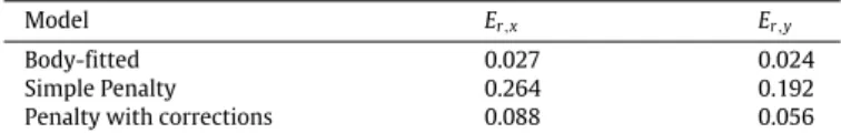
Table 3

Relative error E¯r,k obtained with the fine grid (Grid 3), for both velocity

components.

Model Er,x Er,y

Body-fitted 0.027 0.024

Simple Penalty 0.264 0.192

Penalty with corrections 0.088 0.056

Table 4

Comparison of the drag coefficient and re-circulation length obtained with the fine grid (Grid 3) in a steady-state with literature data.

Model CD LS

Coutanceau and Bouard (Exp.) [45] – 2.13

Tritton (Exp.) [46] 1.59 –

Taira and Colonius [47] 1.54 2.30

Xu and Wang [48] 1.66 2.21

Parussini and Pediroda [49] 1.55 2.27

Body-fitted 1.60 2.31

Simple Penalty 1.58 2.21

Penalty with corrections 1.60 2.30

3.1. Accuracy study with a Wannier flow

The order of accuracy of our Penalty based IBM is first verified with a simple 2D flow in the Stokes regime. The analytical solution of a flow around a circular cylinder, in the vicinity of a moving wall, has been derived by Wannier [43], for very low Reynolds number. The existence of an analytical solution allows a precise comparison with the numerical estimations. The case considers a cylinder of diameter D, centered in a domain of length 6D and height 3D. The dimensions of the problems are presented at the correct scale in Fig. 4. The bottom wall, located at a distance of 0

.

5D to the bottom of the cylinder, is a moving wall with a constant velocity U

=

1 m

·

s−1_{. On all other boundaries the velocity also} satisfies a Dirichlet condition with the analytical solution. A zero gradient condition is imposed for the pressure at every boundary, except at the top wall for the sake of symmetry, where a Dirichlet condition is used.

As an analytical solution is known, the error between the nu-merical and analytical solutions can provide a good estimation of the accuracy of the method. The latter is computed through the normsL₁,L₂andE

¯

r,k, as defined in Eqs.(22)–(24)respectively.

EL1,k

=

1 Nc

∑

i

|

ui,k

−

v

i,k

|

(22) EL2,k

=

( 1 Nc

∑

i

|

ui,k

−

v

i,k

|

2)0.5 (23)

¯

Er,k

=

∑

i⊂ ˜_Ω (

|

ui,k

−

v

i,k

|

|

v

_i,k

|

)si (24)

where uiand vistands respectively for the numerical and analyti-cal solutions computed at the center of the ith cell, k is the velocity

(a) Simple penalty. (b) Penalty with corrections.

Fig. 5. Streamlines of the flow around a cylinder obtained with the coarse grid (Grid 1). The red lines show the position of the extracted velocity profiles.

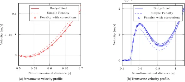
(a) Velocity profiles along the line 1. (b) Velocity profiles along the line 3.

Fig. 6. Streamwise (in red) and transverse (in blue) velocity profiles along sampling lines 1 and 3 near the fixed cylinder. The results are obtained with the fine grid (Grid

3). The vertical black line depicts the position of the cylinder interface. (For interpretation of the references to color in this figure legend, the reader is referred to the web version of this article.)

component, and Ncis the total number of grid cells. The normsL1 andL₂represent global values computed on the whole domain, while the relative errorE

¯

r,kis averaged on a square domainΩ

˜

of size 0

.

6D around the immersed object, and provides an estimate of the local error. In Eq.(24), sistands for the surface elements inside

˜

Ω. The normsL1 and L2 of the errors, obtained with different models, are listed inTables 1and2respectively, for both velocity components. The orders of the different models are estimated using the Richardson method [44]. This method is based on the ratios of the considered values obtained for three different grid refinements. The Grid 1, Grid 2 and Grid 3 considered here, include respectively 10, 20 and 40 cells in the cylinder diameter. The local errorsE

¯

r,kare listed inTable 3for the finest grid.

The corrections of the boundary conditions for velocity and pressure at the interface are shown to achieve a significant de-crease of the normsL₁ and L₂ of the global errors, which are brought to a similar level than body-fitted errors. The local error in Table 3is also reduced from a factor 3 between the simple and the improved penalization methods. Although second-order schemes are used for all simulations, one can note that the overall order of accuracy for the global errors are relatively low. This is probably due to an over-constraint on the boundary conditions on the outer domain. However a qualitative comparison is still

relevant and shows an important increase in the order of the penalization method, which goes approximately from 0.5 to 1.5 when velocity and pressure corrections are accounted for. Finally, the fact that the corrected IBM method achieves a larger order than obtained with the body-fitted approach for a fairly similar error on the fine mesh, can be attributed to a lower accuracy on a coarse mesh.

3.2. Fixed cylinder in a cross flow

In this test case, a fixed cylinder in a 2D cross flow is considered. The domain is rectangular, with a length of 40D and a height of 30D, where D is the diameter of the cylinder. The center of the cylinder is placed at (10D, 15D). On the top and bottom walls a slip-condition is imposed, while inflow and outflow boundary conditions are fixed at the left and right boundaries respectively. A Reynolds number of 40 is considered. The same three grid re-finements relatively to the cylinder, as for the Wannier flow, are used for this case (Grid 1, Grid 2 and Grid 3). This case has been widely studied and used for validation in literature.

The comparison focuses on the drag coefficient CD and the re-circulation length LS behind the cylinder evaluated from the steady-state solutions. The drag coefficient is computed from the

(a) Streamwise velocity profile. (b) Transverse velocity profile.

Fig. 7. Velocity profiles along the sampling line 2 near the fixed cylinder. Results obtained with the fine grid (Grid 3). The black line depicts the interface position.

(a) Local orders of accuracy along line 2. (b) Local orders of accuracy along line 3.

Fig. 8. Local order of accuracy for the velocity along the lines 2 and 3. 20 sampling points were considered for the estimation of the orders. The vertical black line depicts

the position of the cylinder interface.

estimation of the force exerted by the fluid as described in Sec-tion2.1.5. Both physical parameters obtained in previous pub-lished experimental and numerical work focusing on IBM are compared with results from the present penalization method and the equivalent body-fitted simulations (seeTable 4). For a similar resolution near the interface (∆x

=

0

.

025D for grid 3,∆x

=

0

.

05D for Xu and Wang, and∆x

=

0

.

02D for Taira and Colonius), the two physical parameters obtained with the current penalization approaches are in good agreement with what can be found in literature. More precisely, one can note the improvements made by the corrections for the Penalty method, which increase both the drag and the specific length, in accordance with the body-fitted results.

The streamlines of the flow obtained with the present sharp pe-nalization method are shown inFig. 5. As in reality the penalization coefficient (in Eqs.(3)and(5)) is not exactly equal to 0, the zero Dirichlet condition on the immersed interface in this case is not satisfied up to the machine accuracy. As a result, the streamlines may penetrate the immersed solid as shown for the simple Penalty

approach. The improvements on the interface boundary conditions obtained with the corrected Penalty formulation are visible on the same Figure, as they reduce significantly the penetration of the streamlines inside the body. In addition, velocity profiles are extracted along the lines marked in red in Fig. 5. These lines make respectively an angle with the vertical axis of

−

45◦

, 45◦

and 70◦, which correspond to a location where the boundary layer is developed (line 1), a location after the separation point (line 2), and finally a location crossing the re-circulation bubble (line 3). The corresponding velocity profiles are shown inFigs. 6and7, for both streamwise and transverse components. Moreover, for a sake of visibility in the comparison, some zooming were performed on the region close to the interface.

Fig. 6(a)shows the velocity profile before the separation point, where the boundary layer is still attached. As the main issue in this problem is actually for a numerical model to determine the right lo-cation of this separation point, all the approaches lead as expected to similar profiles at this location. After the separation points how-ever, the profiles detailed inFigs. 7and6(b)show the significant

Fig. 9. Pressure contours around the oscillating cylinder for a phase angleωt = 180◦

, obtained with the simple Penalty approach on the medium grid (Grid 2). The white lines show the position of the extracted velocity and pressure profiles.

improvements with the improved penalization compared to the first order approach. These conclusions are consistent with the numerical estimation of the re-circulation lengths, for which the simple Penalty method is giving a significant discrepancy with the body-fitted estimation (around 5%), while the Penalty approach, with both velocity and pressure corrections, has shown to be a more accurate model.

Fig. 8shows locally the order of accuracy for the two velocity components computed with both simple and improved IBM. The orders are estimated along the lines 2 and 3 (seeFig. 5) with the Richardson method [44], using an additional level of refinement for the finest grid. The different curves exhibits a high variability of the order near the interface. Although the first sampling point shows a low order for the two Penalty approaches, the average order of accuracy is above 2 for the Penalty with corrections at a dis-tance of one radius from the interface. Considering the streamwise component, away from the interface, the values seem to converge asymptotically towards 2 for the improved IBM, and towards 1 for the standard IBM. Similarly for the transverse component of the velocity, the order stabilizes between 1.5 and 2 for the improved IBM depending on the sampling line. One can note that the orders outline an higher variability for the transverse component. In ad-dition, the local orders obtained for the simple penalty approach along line 2, which is in the vicinity to the separation point and on the edge of the recirculation bubble, are negatives in some parts. It could be the case that between two grid levels, the sampling line is passing inside or outside the recirculation zone, which would

affect significantly the extracted velocity magnitude. An extra level of refinement might be then necessary to obtain consistent orders of accuracy. This issue is corrected with the improved IBM. These results emphasize the improvements brought by the corrections. Furthermore, they are consistent with the orders of accuracy found for the recirculation length for instance (1.0 for the standard IBM and 1.5 for the improved IBM). The orders obtained with the current Penalty approach with boundary treatments are compa-rable to previously published sharp IBM offering improvements to tackle the rasterization effect. Hence, the penalization method of Introïni et al. [17] leads to a global order of accuracy around 1.88 for the Taylor–Couette problem for both L∞ and L2norms, while global orders between 1.27 and 2.31 are obtained for the flow around a static cylinder, or between 1.51 and 1.91 for the flow around a rotating cylinder. Similarly, the sharp IBM of Gilmanov et al. [50] reaches 1.48 and 1.74 as a global order for the norms L∞and L2respectively when studying the steady flow in a cubic lid-driven cavity. One can also mention that already existing high-order IBM can achieve perfect second-high-order or above for specific test cases [42,16,51].

3.3. In-line oscillating cylinder in a fluid at rest

A cylinder oscillating in a fluid at rest is considered in this case. The dimensions of the problem are similar to the previous test case, as well as the IBM and body-conforming grids used for the simulations. In the standard body-fitted approach, the cells are slightly and smoothly stretched in time, in order to follow the motion of the cylinder. The equation of motion reads: x(t)

=

−

Asin(

ω

t), where the frequency f

=

ω

2π is set to 0

.

2 Hz and the amplitude A is fixed to₂5_π. This motion corresponds to a Reynolds number equal to 100 and a Keulegan–Carpenter number equal to 5. The oscillating cylinder case is a validation case also frequently used in literature [51–54] for numerical model handling moving geometries. Laboratory experiments have been conducted as well by Dütsch et al. [55]. The oscillations of the cylinder lead to the development of lower and upper boundary layers, which separate and generate two counter-rotating vortices in the lee. This genera-tion process stops when the cylinder starts to move backward and finally splits the vortex pair.

The pressure contours obtained with our simple Penalty ap-proach are plotted inFig. 9for a phase position

ω

t

=

180◦

, when the cylinder is in its central position and is moving to the right. The

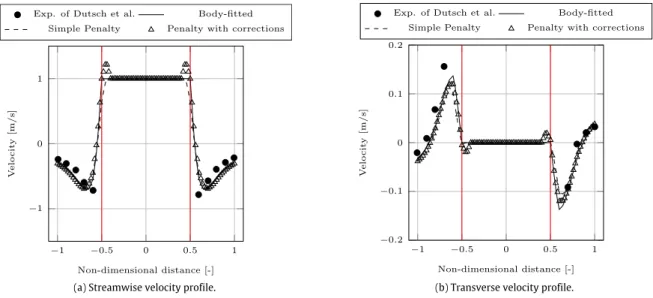
(a) Streamwise velocity profile. (b) Transverse velocity profile.

Fig. 10. Instantaneous velocity profiles near the oscillating cylinder, at x=0 and for a phase angleωt=180◦

. The results are obtained with Grid 2. The vertical red lines depict the position of the cylinder interface.

(a) Profiles at x= −0.6D. (b) Profiles at x=0.6D.

Fig. 11. Instantaneous velocity profiles near the oscillating cylinder, at x=0.6D and x= −0.6D and for a phase angleωt=180◦

. The results are obtained with Grid 2 for streamwise (in red) and transverse (in blue) component of the velocity. (For interpretation of the references to color in this figure legend, the reader is referred to the web version of this article.)

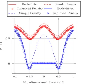
(a) Pressure profiles at x=0 (in blue) and x= −0.6D (in red)

(b) Pressure profiles at x=0.6D.

Fig. 12. Instantaneous pressure profiles along the three sampling lines near the oscillating cylinder for a phase angle_ωt=180◦

. The results are obtained with Grid 2. (For interpretation of the references to color in this figure legend, the reader is referred to the web version of this article.)

pressure is normalized in terms of the cylinder maximum speed Umas p∗

=

p

/

(

ρ

Um2). The pressure contour shows the symmetry obtained with our model, and are in good agreement with the results of Dütsch et al. [55]. On this figure, the white lines represent the position of the extracted velocity and pressure profiles at the same phase angle, respectively at a distance x

= −

0

.

6D, x

=

0, and x

=

0

.

6D from the center of the cylinder. At this time, the cylinder is back to its initial central position, for which the body-fitted mesh is not stretched, allowing for a more relevant comparison with the IBM results.

The improvements brought by the corrected Penalty approach are especially visible near the interface for both streamwise and transverse velocity inFig. 10, where a very good agreement with the equivalent body-fitted is obtained. This especially the case for the magnitude of the transverse velocity peaks. For the two other profiles on both sides of the cylinder inFig. 11, the penalization

approach leads to satisfactory results as well. The experimental results of Dütsch et al. are not shown here for a quantitative valida-tion, but only for comparison purpose. The profiles obtained with IBM are consistent with the experimental velocities and show thus that the qualitative features of the flow are well captured. Further-more, similar level of discrepancies with these experimental data are obtained with other numerical models in literature [51,54].

Regarding the pressure, one can observe that the imposition of the Neumann condition improves the results near the interface on the profile crossing the cylinder (x

=

0) inFig. 12(a). For the two other profiles, although the magnitude is slightly under-estimated,

Fig. 12 shows a better distribution of the pressure around the cylinder for the penalization model with corrections. This result supports the fact that the drag is correctly estimated in this case, and implies as well that the pressure gradient are very similar between the body-fitted and the corrected Penalty method.

Fig. 13. Outline of mixer layout dimensions and CAD rendering view. The static and rotating zones are specified for the body-conforming approach.

(a) Linear reconstruction. (b) Power-law reconstruction.

Fig. 14. Sketch of the velocity correction schemes used for the turbulent case. The same nomenclature is used for the cells definition.

(a) Body-fitted. (b) IBM.

Fig. 15. Contour of the velocity magnitude on a cross-section downstream of the impeller at y=0.1 m for both body-fitted and IBM computations.

3.4. Mixing in a stirred-tank 3.4.1. Case description

This case concerns the cylindrical mixing tank with 4 vertical baffles and the 4 pitched blade impeller studied by Ge et al. [56]. The results reviewed here refer to the 45◦

pitch impeller with rect-angular blades. The tank and impeller assembly has a 90◦

rotational periodicity. Ge et al. study provides both experimental and com-putational results. Radial and axial velocities have been measured using PIV along two radial sampling lines located upstream and

downstream of the impeller at axial position y

=

0

.

09 m and y

=

0

.

13 m and offset by 5◦

from the vertical plane containing the baffles. In addition, the phase averaged turbulent kinetic energy is estimated from the 2D planar PIV measurement using the pseudo-isotropic assumption: k

=

3

4(u

¯

′2

_{+ ¯}

v

′2_{), whereu}

¯

′_and

_v

¯

′_{are the}

turbulent radial and axial velocity fluctuations.

The design of the problem is shown inFig. 13. The tank used in the experimental study was deeper than in the computational model where the height H corresponds to the level of the free surface in experiments. The impeller rotational speed is set at N

=

(a) Body-fitted. (b) IBM.

Fig. 16. Contour of the velocity magnitude on a cross-section cutting the impeller at y=0.11 m for both body-fitted and IBM computations.

Table 5

Numerical settings for the different CFD models.

Model Turbulence model Max. grid res. Impeller thickness Ge et al. RANS k−ϵ 2 mm 0

Body-fitted DDES 0.5 mm 2 mm IBM coupled IBM–DES 1 mm 1.6 mm

Ω

/

2

π

giving the Reynolds number Re

=

ND2

_{/ν =}

₅

_.

₁₈

_·

₁₀4_and the Froude number Fr

=

N2D

/

g

≃

3

.

6. Under these conditions distortions of the free surface by the liquid stirring can be expected to have little influence [57]. Computational tests were conducted with a Volume of Fluid (VOF) model to account for the influence of the free surface and confirmed this to be the case.

3.4.2. Meshing details and accurate turbulence modeling

The computational results from [56] were obtained from a RANS k

−

ϵ

model and a GGI method to handle the rotating zone and a hy-brid mesh. Hexahedral cells were used for the stationary zone and tetrahedral cells ranging from 2 mm in the impeller discharge re-gion to 6 mm elsewhere. Zero thickness baffles and impeller blades were used to avoid meshing complication. Similarly for the body-fitted simulations performed in this research, the Generalized Grid Interface (GGI) method was used to model the moving boundaries. However, a cubic mesh was employed for both the stator and the rotor parts. The edges of the quadrilateral cells are aligned with the coordinate axes everywhere except in the vicinity of inflation layers at wall boundaries where tetrahedral and pyramidal cells are used to make the transition. Local refinements are achieved by dividing cells into uniform octants. The body-fitted mesh is based in the end on 2 mm cells. A refined zone is defined in the rotating region, extending from its lowest point (seeFig. 13) to 0.19 impeller diameter. Finally, one additional refinement is applied in four layers adjacent to wall boundaries. Meshing of the impeller wall relies on a single quad based prism layer (inflation layer). Concerning the impeller itself, a 2 mm wall thickness was used instead of the zero thickness from Ge et al. With this settings, an average y+

of 5.8 was obtained. A coarser mesh was also considered without the intermediate refined region. Finally for the IBM case, a similar cell size was considered in the tank. However, the refined region with 1 mm cells is smaller in this case, ranging from y

=

0

.

095 m to y

=

0

.

13 m. In this sense the equivalent IBM resolution is in-between both body-conforming grids. The IBM is using the physical thickness of the impeller (1.6 mm), hence its discrete representation is only one or two cells thick. The grids details are listed inTable 5.

The impeller surface mesh is composed of triangular elements of 0.25 mm in average, which is four times smaller than the size of the fluid cell. The approximation made for the estimation of the distance to the interface in arbitrary geometry, that is which cannot

Table 6

Volume averaged relative error as defined in Eq.(25)for different methods of com-puting the distance to the immersed interface.

Method Dicho. 5 it. Dicho. 10 it. Dicho. 20 it. surface mesh

ErrorE¯d 0.25 0.0059 5.2e−6 0.0085

be defined analytically, is discussed here. We define the average error in the calculation of the distance between fluid cell center points and the interface as:

¯

Ed

=

1

∫

ΩpdΩ

∫

Ωp Ed,idΩ

=

1

∫

ΩpdΩ

∫

Ωp (d(xi)

−

dref(xi) dref(xi) )dΩ (25) where Ed,iis the local relative error in cell i between the approxi-mate distance d(xi) and a reference distance dref(xi). The reference distance is calculated with a dichotomy algorithm using 80 itera-tions. The average error is integrated over the penalized domain

Ωp. The average errors obtained with the considered surface mesh and with different dichotomy iterations are listed inTable 6. Us-ing 20 iterations for the dichotomy algorithm is shown to give a negligible relative error. This support the argument that the error in the estimation of the distance, which converges in 2k_{, k being} the number of dichotomy iterations, is low enough to consider the distance obtained with 80 iterations as the real distance to the interface. From the table, we can see that approximating the distance to the interface by the distance to the closest solid points with a surface mesh of 0.25 mm elements leads to an average relative error below 1%. This can be considered as acceptable for our simulation case. Furthermore, it should be noted that the approximation made here reduces the CPU time for computing the distance from 8.87 s to 2.53 s in comparison to a dichotomy algorithm using 80 iterations. These CPU times were obtained for a sequential simulation and the distances were estimated for all cells in the penalized domains (approximately 20,000 cells in total). The same analysis on the error is performed for the Wannier case, described in Section3.1. The medium mesh is considered (Grid 2) for the fluid domain and here also the surface mesh for the cylinder is composed of triangular elements four times smaller. The reference distance is calculated with the analytical distance to the interface. An average relative error around 2.5% was found in the penalized domain. The larger relative error obtained in this case can be explained by the use of larger volume and surface mesh.

Both body-fitted and IBM simulations performed for this study have used hybrid RANS–LES type of turbulence model. While the IBM is coupled to a DES model (see Section2.3), the body-fitted case used instead the Delayed Detached Eddy Simulation (DDES), which reduces incorrect behavior triggered by a grid spacing par-allel to the wall smaller than the boundary-layer thickness [58]. The resolutions of the two body-fitted grids have been assessed in

(a) Body-fitted. (b) IBM.

Fig. 17. Q -criterion iso-contours with Q=104_{colored by the magnitude of the velocity.}

(a) Downstream of the impeller. (b) Upstream of the impeller.

Fig. 18. Phase and time averaged axial velocity along the two sampling lines.

terms of the kinetic energy spectra. The results have shown that both mesh are fine enough to fully resolved the inertial range, with a spectrum characterized by a curve of slope

−

5/3. For this type of transient problem involving high speed flows, the PIMPLE scheme is used to solve the pressure–velocity coupling, instead of the PISO scheme introduced before. The PIMPLE scheme is a combination of both PISO and semi-implicit method for pressure-linked equations (SIMPLE) schemes, that enables looping over the entire system of equations and allows the use of larger time step.

The correction scheme for the velocity boundary condition on the interface, introduced in Section2.1.4, has been modified for the mixer case. Due to the small thickness of the impeller blade rela-tively to the mesh size, the velocity corrections are applied within an Eulerian cell layer outside of the solid domain. In this case, the penalized domainΩprefers then to the cells inΩf possessing at least one neighbor inΩs. In this configuration, the reconstruction of the penalized velocity inΩpis based on a linear interpolation in the same spirit as the previously employed extrapolation. Both inner [31,16] and outer [50,42] types of corrections have been considered in IBM studies. However, given the mean y+

obtained with the body-fitted simulation, it can be assumed that cells ad-jacent to the impeller boundaries will typically be placed in the

logarithmic layer provided that the flow remains attached, when modeled with IBM. For this reason, a velocity correction scheme based on a power-law is also considered in order to better describe the turbulent velocity profile of the boundary layer. Similar types of corrections have been proposed by Choi et al. [59] and Chang et al. [60] for turbulent flows. A 1/7 power law was firstly proposed by Werner and Wengle [61]. In [60], Chang et al. have considered and compared both linear and power-law based reconstruction of the velocity. Their results suggest that the former method gives slightly better results, and the authors argue that this is most likely due to the high level of grid refinement used, which is fine enough to reach the viscous sub-layer in some areas.

The velocity correction scheme based on linear interpolation is formulated in Eq.(26). This correction is performed in the same spirit as the inner extrapolation scheme described in Section2.1.4. The definition of d1, d2and uφare identical. The linear interpolation is illustrated inFig. 14(a).

u∗ p

=

d2

−

d1 d2 uib,n

+

d1 d2 u_φ

.

(26)

For the power-law interpolation, the reconstruction is formu-lated similarly to the tangency correction of Choi et al. [59], by de-composing the velocity into its tangential and normal components

(a) Downstream of the impeller. (b) Upstream of the impeller.

Fig. 19. Phase and time averaged radial velocity along the two sampling lines.

(a) Downstream of the impeller. (b) Upstream of the impeller.

Fig. 20. Phase and time averaged turbulent kinetic energy along the two sampling lines.

relatively to the immersed surface: u∗

p

=

uT

+

uN

+

uib,n. In this formulation, uTand uN are the components of the fluid velocity relative to the wall velocity. The dependence of the tangential component uTto the normal distance to the wall is assumed to follow a power-law function. In this case, the tangential velocity at the cell center P can be derived from the tangential velocity at a virtual point

φ

as:

uT

=

( d1 d2

)ku_φ,T (27)

where small values of k (usually 1/7) can approximate the loga-rithmic distribution expected in the near wall region for an at-tached turbulent flow. The normal component of the velocity uN is assumed to follow a linear distribution, i.e. using k

=

1. The reconstruction of the tangential velocity component is illustrated inFig. 14(b). The body fitted simulations indicate that the wall adjacent cells along the impeller lie well within the inner layer of

an attached boundary layer with an average y+

of 5.8. As the IBM mesh size is twice that of the body fitted version, the penalized point P determined in terms of the distance d1from the immersed interface can be expected to be typically located somewhere in the buffer layer, but this will change as the interface moves over the underlying Eulerian grid. Rather than reproducing the different parts of a fully-developed turbulent boundary layer, the inner layer (from the viscous sub layer to the overlap layer) is approximated by the power-law as implemented for example in [61] for y+

_>

11

.

8 or in [59] for the whole layer. This means that the boundary correction does not impose the turbulent boundary layer profile as a function of y+

and a single reference point is sufficient to reconstruct the full profile irrespective of its location within the boundary layer. The main assumption used in this case is that the velocity at the virtual point (at a distance d2) does fit the power law, which is incorrect if the flow departs from the zero pressure gradi-ent boundary layer condition. Imposing this reconstruction does in

Fig. 21. Contours of the velocity, projected in the direction of the impeller rotational speed (+z), obtained with a linear reconstruction at the immersed surface. The contours

are shown on cross-sections perpendicular to two impeller blades diametrically opposed. The white contours depict the impeller surface.

Fig. 22. Contours of the velocity, projected in the direction of the impeller rotational speed (+z), obtained with a power-law (k=1/7) reconstruction at the immersed surface. The contours are shown on cross-sections perpendicular to two impeller blades diametrically opposed at a distance of 0.06 m from the impeller center of rotation. The white contours depict the blades surface.

such a case promote boundary layer attachment by imposing the attached velocity profile at the immersed boundary cell. The next sections present the results obtained with a linear reconstruction of the velocity, while Section3.4.5discusses the sensitivity to the type of reconstruction.

Finally, regarding the dependence of the turbulence viscosity to the distance to the wall, Prandtl’s assumption [62] is usually used for the logarithmic layer, for which the non-dimensional turbulent viscosity is directly proportional to y+

. In this context, the present linear reconstruction of the turbulent viscosity in the penalized domain, as used also by Balaras [42] is relevant. For the body-fitted simulations, Spalding’s law [63] is used to compute the local turbulent viscosity in order to get the proper wall shear stress. This wall function is valid for all-y+

and was developed for attached boundary layers.

3.4.3. General results

The initial conditions for the simulation were based on a fluid at rest with uniform static pressure distribution gravity being ne-glected. The velocity contour obtained after 5 impeller revolutions are shown in Figs. 15and 16. The accuracy of this variable is meaningful for mixing problems. In the considered areas, the mesh size is∆x

=

1 mm in a circular region centered in the impeller with a radius of respectively 0.11 m for the body-fitted case and 0.08 m for the IBM case, while the mesh size is∆x

=

2 mm outside these regions. Although the regions of high velocity magnitude look more heterogeneous directly below the impeller inFig. 15, the current penalization approach is leading to a similar level of mixing in the tank, as confirmed by the time averaged flow velocity

profiles discussed in the next section (Section3.4.4). The size of the dead zone directly under the impeller as well as the extend of the zone characterized by high downstream velocity are in good agreement with the body-fitted case. For the plane cutting the impeller inFig. 16, the extend of the region of high velocity swept by the impeller also show generally similar characteristics in terms of their spread and diameter. There is however some non negligible difference in the intensity and length of the wake trailing behind each impeller blade. The high velocity region is shown to spread further radially downstream of the impeller (at y

=

0

.

1 m) in the IBM case with a lower velocity magnitude, while the flow remains attached to the impeller for longer with the body-fitted mesh allowing for higher velocity flow to evolve which then diffuses more rapidly in the wake, as it can be seen inFig. 17. This figure highlights the turbulent structures predicted by the models in terms of the Q -criterion. Q is defined by 1

/

2(Ω2

₋

_S2_{), where} S

= ∥

1

/

2(

∇

u

+ ∇

T_u)

_∥

_andΩ

_{= ∥}

_tr(

_∇

_u)

_∥

_{are the strain rate and} vorticity rate magnitudes, so that positive iso-contours represent vortices defined as a region where the vorticity is greater than the magnitude of the strain rate.

Concerning turbulence modeling, it is worth noting that the penalization of the turbulent viscosity is a necessity when using a full RANS model. Without a correct boundary condition on the immersed interface, the turbulent viscosity computed inside the solid from the Spalart–Allmaras equation can be very high, leading to an overestimated diffusion in the flow. The influence of this pe-nalization process is however found to have a negligible influence when a DES turbulence model is used. Results confirm that with DES models a correct estimation of the turbulent variables in the