Technology researchers and makes it freely available over the web where possible.
This is an author-deposited version published in: https://sam.ensam.eu Handle ID: .http://hdl.handle.net/10985/7318
To cite this version :
Rezki CHEBLI, Olivier COUTIER-DELGOSHA, Bruno AUDEBERT - Development of algorithm based on the fractional time step for the simulation of cavitation. - 2013
Any correspondence concerning this service should be sent to the repository Administrator : [email protected]
1
Development of algorithm based on the fractional time
step for the simulation of cavitation.
R.CHEBLIa,b, O. COUTIER-DELGOSAHa, B. AUDEBERTb
a. Laboratoire de Mécanique de Lille (LML) / Arts et Métiers PariTech, 8 Boulevard Louis XIV, 59046
Lille, France.
b. EDF R&D, Département Mécanique des Fluides Energies et Environnement, 6, quai Waiter, PB 49, 78401 Chatou, France.
Résumé:
La cavitation est l’un des phénomènes physiques les plus contraignants influençant les performances des machines hydrauliques. Il est donc primordial de savoir prédire son apparition et son développement, et de quantifier les pertes de performances qui lui sont associées. L’objectif des simulations numériques est de prédire les instabilités liées à la présence de la cavitation. Le but de ce travail est de développer un algorithme semi-compressible cavitant basé sur la méthode de pas fractionnaire dans le Code_saturne. Un solveur implicite en pression, basé sur une équation de transport d’un taux de vapeur couplée avec les équations de Navier-Stokes est proposé. Un traitement spécifique aux termes sources de cavitation permet d’obtenir des valeurs physiques du taux de vide (entre 0 et 1) sans les limiter numériquement. L’influence de la turbulence est également étudiée. Pour cela, plusieurs modèles de turbulence sont testés et comparés. On cherche en particulier à analyser les effets tridimensionnels intervenant dans les mécanismes d’instabilité. Ce travail nous permet d’aboutir à un outil numérique, validé sur des configurations d’écoulements cavitants complexes, afin d’améliorer la compréhension des mécanismes physiques qui contrôlent les effets instationnaires tridimensionnels intervenants dans les mécanismes d’instabilité.
Abstract:
Cavitation is one of the most demanding physical phenomena influencing the performance of hydraulic machines. It is therefore important to predict correctly its inception and development appearance, and quantify the performance losses associated with it. The objective of the simulations is to predict the instabilities associated with the presence of cavitation. The aim of this work is to develop a semi-compressible cavitating algorithm based on the fractional step method in Code_saturne. An implicit solver, based on a transport equation of void fraction coupled with the Navier-Stokes equations is proposed. Specific treatment of cavitation source terms provides physical values of the void fraction (between 0 and 1) without any numerical limitation. The influence of the turbulence models is also studied. To do this, several turbulence models are tested and compared. The instabilities due to three-dimensional effects are particularly analyzed. This work allows obtaining a numerical tool, validated for complex cavitating flows configurations, in order to improve the understanding of the physical mechanisms that control the three-dimensional unsteady effects involved in the mechanisms of instability.
1
Introduction:
Cavitation is a phenomenon that is responsible for the appearance of vapour in a liquid subjected to a depression. A semi-compressible cavitating algorithm, based on fractional step method implemented in Code_saturne, is presented in the present paper. An implicit solver, based on a transport equation of void fraction coupled with the Navier-Stokes equations, is proposed. Specific treatment of cavitation source terms provides physical values of the void fraction (between 0 and 1) without any numerical limitation. The influence of the turbulence models is also studied. For that purpose, several turbulence models are tested and compared.
2
2
Cavitation modelling:
The internal structure of the two-phase flow is extremely complex and variable, particularly in the case of cavitation. The precise motion and size of small bubbles are often unknown. In addition, the computational resources do not enable to capture all bubble interfaces, because this would require a huge number of cells. This is why the structure of both phases is considered at a macroscopic scale. (COUTIER-DELGOSHA et al, 2007). It means that each cell contains a portion of liquid and a portion of vapour. The proportion of liquid and vapour in this cell is defined macroscopically by defining a void fraction:
α= Vapour volume
Total volume ( 2.1)
We may define physically here a ‘two-phase fluid particle’ which volume V is much larger than the thickness of the liquid/vapour interfaces, but also much smaller than the characteristic scales of the flow. It is assumed that there is no slip between vapour and liquid phases. The flow is considered as a homogeneous fluid that is modelled across the control volume V. The mixture density is given by:
= + 1 − ( 2.2)
and are densities of vapour and liquid phases respectively. The system to solve is:
+ ∇ ρ U" = 0 ( 2.3) ∂ ∂t U" + ∇ % U&' = ∇ π ( 2.4) ∂α ∂t + ∇ α U " = Γ ( 2.5)
ρ is the mixture density, U is the mixture velocity, Γ is the cavitation source term and
π
is the tensor for the external forces.3
Resolution method:
The proposed algorithm is based on the fractional step method. This is one of the methods that allow numerical resolution of the Navier-Stokes equations by decomposing their operators into less complex ones using sub-intermediate steps in the same time step (Guermond, 2006).Two sub-steps are performed: the first one treats the convective and diffusive parts as well as source terms of the momentum equation. It constitutes the velocity prediction step. The second sub-step, known as pressure correction or velocity projection step, resolves the mass equation.
3.1
Velocity prediction step:
The first step is to solve the momentum equation. Shifted discretization with a first-order temporal scheme is applied to the unsteady term and the pressure is treated explicitly.
|Ω)| ∆ )+,∗)− )+./,+) + 0 1 ρU 2 U∗ 345 645 5 7 +849:;<=>? ) − 0 1 µ grad U∗ 345 645 5 7 +849:;<=>? ) = − grad P2 C+ ST ( 3.1)
3
|Ω)| is the volume of the cell (I), U∗ is the predicted velocity, 645 is the common surface between cells (I) and (J), µ is the dynamic viscosity, P is the pressure, ∆ is the time step and ST is the source term. The index (n) refers to the previous time step.
3.2
Pressure correction step:
The equation for pressure correction is obtained by subtracting the equation of velocity prediction, already resolved at previous step, from the momentum equation written with an implicit pressure.
div F|Ω∆
)| )+ grad GH CI = div ,
+J/)− KLM ,∗)
( 3.2)
A pressure increment (δP), which is equal to the pressure difference between the time n+1 and n, is obtained at the end of this step.
Under the assumption of non-compressibility of pure vapour and pure liquid phases (ρN and ρO are considered as constants), the velocity divergence may be written as a function of the cavitation source term.
div U " = Γ ρ/ P−
/
ρQ) ( 3.3)
A Rhie & Chow filter is applied here to avoid the decoupling of even and odd cells on a Cartesian grid, which is due to the cell pressure gradient presented in the predicted mass flow and which is inherited from the prediction velocity step (C. Rhie, 1983.).
0 1 R ϵ 2STUVWXYZ[ C ρ∆t C 2 grad δP \]^ 3 STR = 0 1 R ϵ 2STUVWXYZ[ C U∗+ α _Z`a ρ∆t C 2 grad P2 bSNN 3 STR − α_Z`a 0 1 R ϵ 2STUVWXYZ[ C ∆t ρC2 grad P2 \]^ 3 STR+ ΓCc 1 ρO− 1 ρNd |ΩC| ( 3.4)
α_Z`a is the Arakawa coefficient and fTR is the face between cells (I) and (J) through which the gradient is calculated.
Discretization of the cavitation source term fg :
In most works (R. F. Kunz, 1999), (I. Senocak, 2004), the cavitation source term Γ is expressed in vaporisation and condensation terms, mhJand mh. respectively. These terms are obtained either from the dynamic interface between the two phases or from a derived form of Rayleigh-Plesset equation describing the dynamics of bubbles in a two-phase flow. Therefore, they often depend on the pressure and void fraction α.
Γ= mh.+ mhJ = f α , P ( 3.5)
Temporal discretization of the source term Γ has a major role in the convergence and stability of calculation. An explicit treatment of the pressure generates intense instabilities which lead to divergence of the calculation. To avoid these problems, the pressure is treated implicitly using the Taylor expansion. The aim of this treatment is to damp the instabilities observed during the resolution of the pressure correction equation.
4
ΓC= ΓC+ H+, α+ + ΓC
+ H+, α+
H GH) ( 3.6)
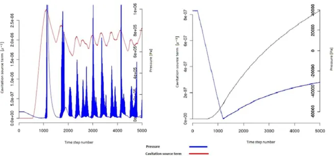
A new term containing the pressure increment GH appeared then in the right hand side of the pressure equation, this term will be added to the resolution matrix diagonal. The equation can finally be solved implicitly. FIG. 1 displays the instabilities obtained when an explicit algorithm is applied (left side figure), and the decrease of these instabilities when the implicit algorithm is used (right side figure).
FIG. 1: – Cavitation source term and pressure evolution using explicit or implicit algorithm.
3.3
Solving of void fraction transport equation step:
The final step is the resolution of the void fraction transport equation. First, a special treatment for the cavitation source term is proposed. This treatment allows obtaining physical values of the void fraction (between 0 and 1) without forcing numerically their limits (maximum/minimum principle of the void fraction). The idea is to multiply the cavitation source term by 1 α × 1 − α 3. This treatment leads to constraints on the time step to meet this principle. Application of an upwind convection scheme results in the following two conditions on the time step:
1 + ∆ 1 − α F ΓC+ + ΓC + H+, α+ H GHI ≥ 0 ( 3.7) 1 − ∆ α F ΓC+ + ΓC + H+, α+ H GHI ≥ 0 ( 3.8)
The equation to solve is as follow:
4
Boundary conditions and turbulence modelling:
Two types of geometry are tested: A 2D Venturi type section and a 2D foil section. The Venturi is 1.272 m long, its inlet section is 0.044 m wide and 0.05m high, and its divergence angle is 8°. The foil is a NACA66 with a chord length of 0.150 m, a span of 0.191 m, and the incidence angle is 8°.
|Ω)|
∆ +J/)− +) + 0 1 U 2 α2J/ 345 645 5 7 2STUVWXYZ[ )
5
Validation of the results is based on the oscillation frequency and the mean attached cavity measured in previous experiments in both configurations. The influence of the mesh size on the Strouhal number has been studied to perform mesh-independent calculations. 2D and 3D simulations were performed. The 2D mesh of the Venturi contains 99000 elements (79000 elements for the foil), whereas the 3D mesh has 3400000 (the foil has 5200000). For the boundary conditions, we assume that no cavitation appears in the inlet and the outlet areas. An inlet velocity ,4+ 8n = 7.2 r/t and an outlet cavitation number σ = 2.6 are imposed. The cavitation number is defined as: w = |.} ~x. xyz{
•€•‚•ƒ„… , where H†‡ is the
vapour pressure at 20°C. Several turbulence models, based on the Reynolds-Averaged Navier-Stokes equations (RANS), are tested to study the influence of this parameter on the results. The first model tested is the two-equation k − ε model. This model does not lead to good results; it has been modified using the correction of Reboud (J.-L. Reboud et al, 1998), which consists in reducing the turbulent viscosity often overestimated in the mixture. The k − ω SST Model is also tested and modified. Other models which are based on the Reynolds stress’s (RSM) are also tested.
5
Results and discussion:
5.1
Venturi case :
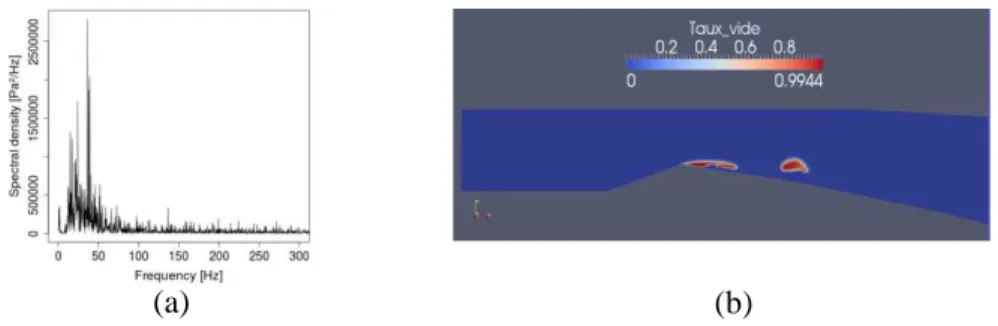
In this case, the time step ∆ = 10.}t satisfies the two conditions shown at section (3.3) and allows obtaining physical values of void fraction [0 1]. All tested turbulent models give an unsteady behaviour and an approximate frequency of 20 Hz (except the standard k − ε model which gives a steady behaviour). In comparison with experiments, in which 45 Hz is observed and therefore a Strouhal number of 0.3, the simulations give a very low Strouhal number (of 0.13). Only the modified k − ε model is able to reproduce the observed experimental frequency with a Strouhal number of 0.3.
FIG. 2 – Cavitating flow simulation, σXYŠNSŠ= 2.6 ,UT2NSŠ= 7.2 m/s, modified k − ε turbulence model. (a) Fast Fourier transform applied to the input pressure signal, (b): void fraction.
FIG. 3 – Cavitating flow cycle, σXYŠNSŠ= 2.6 , UT2NSŠ = 7.2 m/s , modified k − ε turbulence model.
6
5.2
Foil case:
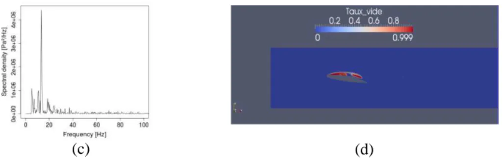
In this case, all tested turbulent models give an unsteady behaviour and seem to agree with experiments, with a slight advantage for the modified k − ε model. This model gives a Strouhal number of 0.3 (13.88 Hz and 0.12 m of the mean attached cavity), whereas experiments give 9.8 Hz of frequency and 0.12 m of mean attached cavity.
FIG. 4 – Cavitating flow simulation, σXYŠNSŠ= 1.3, UT2NSŠ= 5.3 m/s, modified k − ε turbulent model. (c) Fast Fourier transform applied to the input pressure signal, (d): void fraction.
6
Conclusion:
A numerical model based on fractional step method has been developed for the simulation of the cavitating flows. The originality of the present work is the application of two conditions on the time step in order to limit variations on the void fraction in the physical range [0 1]. The results obtained various RANS turbulence models confirm the capability of the modified k-epsilon model initially proposed by Reboud et al (1998) to reproduce unsteady periodical behaviour of the sheet cavity, as well in the Venturi section as on the foil section.
References
[1] C. Rhie, W. C. (1983.). Numerical study of a turbulent flow past an airfoil with trailing edge separation. AIAA J., 21 :1525-1532.
[2] C.L Markle, J. f. (1998). Computational modeling of the dynamics of sheet cavitation. Third Int.
Symposium on cavitation, (p. PP 307 311). Grenoble ,FRANCE.
[3] COUTIER-DELGOSHA et al, O. (2007). Analyse of cavitating flow structure by experimental and numerical investigations. (J. F. Mech., Ed.) 578 (pp 171-222).
[4] COUTIER-DELGOSHA, O. (2001). Modélisation des écoulements cavitants: Etude des
comportements instationnaires et application tridimentionnelle aux turbomachines. Grenoble: INPG.
[5] Delannoy et al. (1990). Cavity Flow Predictions based on the Euler Equations. ASME, (pp. pp. 153-158).
[6] Guermond, J. L. (2006). An overview of projection methods for incompressible flows. Comput.
Methods Appl. Mech. Engrg. 195 (2006) 6011-6045 .
[7] I. Senocak, W. S. (2004). Interfacial dynamics-based modelling of turbulent cavitating fows, Part-1: Model development and steady-state computations. International journal for numerical methods in
fluids , 42, 10.1002/fld. 692.
[8] J.-L. Reboud, B. S. (1998). Two-phase flow structure of cavitation: experiment and modelling of unsteady effects. 3rd International Symposium on Cavitation CAV1998. Grenoble - France.
[9] R. F. Kunz, D. A. (1999). multi-phase cfd analysis of natural and ventilated cavitation about submerged bodies 3rd ASME/JSME Joint Fluids Engineering Conference, FEDSM99-7364, 1999. 3rd
ASME/JSME Joint Fluids Engineering Conference, (pp. FEDSM99-7364).
[10] Robert F. Kunz, D. A. (1999). A preconditioned Navier-Stokes method for two-phase flows with application to cavitation prediction. Computers & Fluids , 29 (2000) 849-875.