Analysis of Soil Variability Measured with a Soil Strength Sensor
B. HANQUET, D. SIRJACOBS AND M.-F. DESTAIN1, M. FRANKINET2, J.-C. VERBRUGGE3
1Gembloux Agricultural University, Unité de Mécanique et Construction, Passage des Déportés 2, B-5030 Gembloux, Belgium 2Centre de Recherches Agronomiques, Département Production Végétale, Rue du Bordia 4, B-5030 Gembloux, Belgium 3Université Libre de Bruxelles, Service de Mécanique des sols, Avenue F. Roosevelt 50, B-1050 Bruxelles, Belgium
Abstract: In the context of precision agriculture, the knowledge of soil strength variability at the field scale may
be useful for improving site-specific tillage. Moreover, rapid and accurate sensing methods for soil physical properties determination would favourably replace labour-intensive, time-consuming and expensive soil sampling and analysis. This study aims at validating conclusions of a previous study which was conducted to develop and test a soil strength sensor in field conditions. The coupled acquisition of the sensor's signals and the corresponding DGPS positions allowed establishment of maps for the three measured outputs, namely the horizontal force (Fx), the vertical force (Fz) and the moment (My). In order to study the relationships between
measured forces and soil physical parameters, a series of soil properties were measured on soil cores collected in 10 reference plots. Significant correlations were found between Fx and the average resistance to cone penetration
at 25 cm depth (r = 0.95) and between Fx and average soil moisture at 30 cm depth (r = -0.95). These
relationships were similar to those found in the first study. This sensing method proved its capability to characterise within-field soil variability.
Keywords: sensor, mapping, soil variability, soil strength, soil physical properties
Introduction
Among crop production factors, the soil is obviously one of the most important. Therefore, within the context of precision farming, the knowledge of its physical and mechanical properties, as well as the spatial variability of these properties, is essential as decision support information for modifying cultural operations. Up to now, data collection on soil is mostly made by grid-sampling to determine, e.g., texture, pF, water content, water
infiltration rate, bulk density, cone index, organic matter and shear strength. Measurements of these properties are labour-intensive, time-consuming and expensive. Thus, the development of sensors suited to quantify soil properties at the scale required for accurately mapping within-field variations is a necessity in order that precision agriculture can be widely practised (Stafford, 2000).
Soil strength is one factor known to influence yield, particularly when a soil has a traffic and/or a tillage hard pan. The most rigorous procedure to measure this property is achieved by performing triaxial tests on cylindrical samples in order to estimate two main mechanical parameters: cohesion and angle of internal friction. One limitation of this method is the difficulty of collecting homogeneous core cylinders having a height equal to two times the diameter in tilled layers (Guerif, 1994). It is also an expensive and time-consuming method.
Assessment of soil strength is often performed by measuring the soil resistance to penetrometer probes: the cone index, which is the applied force divided by the base area of the cone. Cone index is a compound parameter that includes components of shear, compressive and tensile strength, the relative contributions of which are not known. Moreover, when agricultural soils are in an unsaturated state, the shear strength is also largely affected by the moisture content (Fredlund et al., 1978; Verbrugge and Fleureau, 2002). Due to its easy use, the penetrometer is sometimes included in procedures designed to create soil strength maps. However,
understanding the spatial variability of soil strength requires the collection of extremely large amounts of data, which is probably not a cost-effective process at large scale (Clark, 1999).
To overcome this limitation, several authors developed sensors allowing on-the-go measurement of soil mechanical impedance. Lui et al. (1996) measured draft requirements in different soil conditions using the reference tillage tool developed by Glancey et al. (1996). The authors computed a texture/compaction index (TCI), which is a function of draft and soil moisture content. More recently, Adamchuk et al. (2001) developed an instrument for measuring soil resistance at multiple depths at a time (3 depths, down to 30 cm). Acquiring measurements together with GPS positions allowed the authors to create resistance maps. Moreover, they found a high correlation (r = 0.95) between the resistance measured using the implement and averaged cone index values. Andrade et al. (2001) developed a similar sensor which measures the soil's resistance profile to a depth of 63 cm (8 measurements). By means of this profile sensor, the authors showed that cutting force is influenced by
soil moisture content, depth of operation of the tine and vertical location of the cutting element.
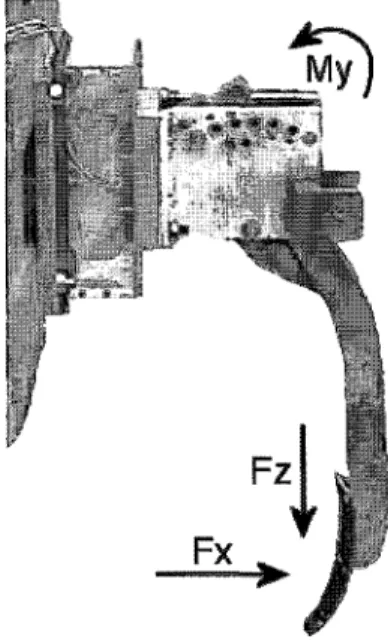
The sensor used in this research was developed by Sirjacobs et al. (2002). It is constituted of a thin blade pulled in the soil at constant depth and speed which transfers the soil blade forces to a transducer fixed on the machine. The transducer is an octagonal ring equipped with strain gages designed to measure the draft force (Fx), the
vertical force (Fz) and the moment (My). The design of this dynamometric ring was based on the work of Godwin
(1975). The sensor acquires continuous information and, when coupled to a DGPS, offers the possibility to draw maps illustrating soil variability. Furthermore, from an experiment conducted on a 2 ha silty homogeneous soil (Hesbaye, Belgium), significant relationships were established between the sensor outputs and reference soil properties, such as a cone index values and the gravimetric water content. However, these relationships were not universal, but limited to specific soil types and conditions present in the field.
The main objective of this study was to check the global methodology of the previous study in a more heterogeneous field. More precisely, the paper attempts to give responses to the following questions: (1) is the sensor suited to distinguish between soil units within a field? (2) is it possible to correlate the measured soil cutting force values to soil physical and mechanical properties? (3) if yes, are these reference properties the same as those focused in the last study?
Materials and methods
Description of the study field
The research site was a 10.7 ha field located near Gembloux (Belgium), owned by a farmer and managed partly by himself, and partly by the Centre de Recherches Agronomiques (CRAGx). This region is situated on the low and feebly undulating plateaux, to the west of the Belgian "silty area".
Soils are exclusively alluvial soils differing by their drainage potential: drainage is good in the eastern part of the field (Abp, in the Belgian classification) and becomes quite poor in the NNW (Ahp). One can also mention the presence of a "textural B horizon" buried at a small depth in the ESE part of the site (Pécrot, 1957).
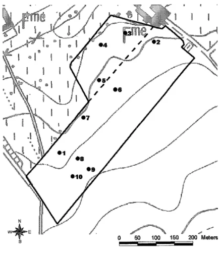
The average slope is small (about 0.015 m/m) and oriented NNW. The difference in altitude between the highest and the lowest points is about 7.5 m. The field can be divided in two parts because of its cultural history
(Figure 1): the part above the dashed line was a pasture a few years ago, while the other part has been cultivated for a longer period of time. The study was conducted after a winter wheat crop, which was harvested on 15 August 2000.
Field campaign
Reference measurements.
A series of reference measurements were obtained in 10 locations within the field on 31 August 2000. The test plots (Figure 1) were not distributed according to a regular grid, but their location was chosen on the basis of a previous preliminary soil strength mapping of the field (March 2000) which indicated severe heterogeneity. The test plots were treated as homogenous soil units and their dimensions were chosen long enough (20 m along the track) to obtain representative mean measurements.
Soil strength measurements.
Soil strength was measured on 31 August 2000 using the on-the-go sensor described by Sirjacobs et al. (2002). The sensor (Figure 2), mounted on the three point hitch of a tractor, was pulled along 46 transects in the field, (transect interdistance: about 7.5 m). The speed was maintained constant at 5.0 kph (based on the tractor's digital tachometer) and the blade depth was adjusted to 30 cm using the hitch position control system. The signal from the sensor was recorded simultaneously with DGPS signal (Omnistar 3000-LR-8) on an industrial laptop using a LabView (National Instruments) self-made virtual instrument. Soil strength measurement rate was 500 Hz. The signal (output imbalance tension of the Wheatstone bridges) was averaged to 1 Hz by post-processing (low-pass filter) and converted to force (Fx and Fz) and moment (My) values using the sensor's linear calibration equations.
The DGPS positions were then assigned to corresponding values of horizontal force (Fx), vertical force (Fz) and
moment (My). Positive values of each force component are directed as shown by arrows on Figure 2. More
Figure 1: Experimental field, topographic map and localisation of the test plots.
Data analysis and interpolation
Continuous maps representing the within-field variation of soil texture and soil strength parameters were produced using the Inverse Distance Weighted algorithm available in the Spatial Analyst module for ArcView (ESRI). Different search radii, depending on the density of the measurements, were used for interpolation: 20 m for soil strength, 30 m for soil texture. An influence factor of 1 was chosen to obtain smooth aspect maps. In addition, statistical analysis was performed using Minitab software to compute matrices of correlation coefficients, linear and multi-linear regressions.
Results and discussion
Field reference measurements
Soil sampling and analysis: permanent soil characteristics.
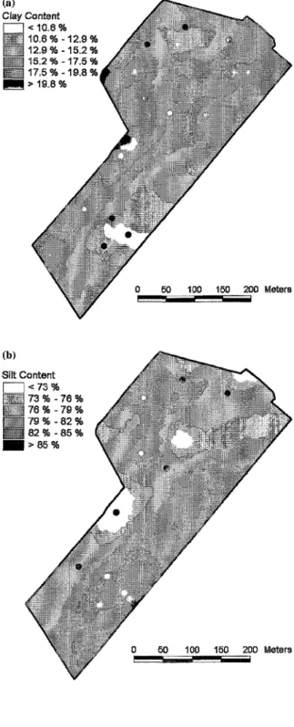
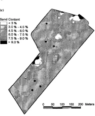
A systematic soil sampling was done to determine soil texture on a 25 m square grid basis over the whole field. Ten soil cores were collected in the top 30 cm layer at 179 points. Sand, silt and clay content were measured for each point. This analysis was performed during August 1999. As soil texture is not subject to quick and
important modifications, data were thought to be still relevant at the time of the experiment. Soil texture data were interpolated to produce maps (see Figure 3) and to determine values corresponding to the 10 plots (Table 1). The mean soil composition was 78.6% silt, 15.2% clay and 6.2% sand. Around these mean values, some variability appeared in the field. Especially, the clay content was lower on the crest (especially near points 8-10, the mean value was around 11 %) than at the lowest elevation. Some zones revealed a low silt content: namely near point 7, where high sand and clay contents (respectively around 13 and 18%) were measured.
Particle-size distribution curves are presented in Figure 4. Measurements were done using conventional sieving and sedimentation techniques and revealed a similar general shape of the curves, even if point 7 presented a sand
content distinctly higher than the average.
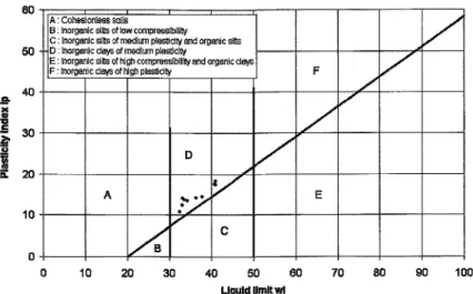
Atterberg limits, liquid limit (wL) and plastic limit (wP), were measured for all the test plots, and the plasticity
index (IP = wL - wP) and consistency index (IC = (wL - w)/IP) were calculated (Table 1). Values of IP ranged from
10% to 20% and showed significant variations between plots. Thus, the water content range in which a plastic behaviour is expected could be considered as "medium". The consistency index, which takes the actual water content (w) into account, was close to 1. Consequently, the soil was qualified as "not very consistent" (plots 3-5, 8-10) to "consistent" (plots 1, 2, 6 and 7).
These parameters can be used to classify soils. Reporting the couple (IP, wL) on a Casagrande diagram indicated
that the studied soils belonged to the "inorganic clays of medium plasticity" class (Figure 5), but were quite close to the limit of "inorganic silts of medium plasticity".
pF curves show similar trends for all the plots, even if curves corresponding to points 3 and 4 on one hand and curve relative to point 7 are quite separate from the set (Figure 6).
Available water content (AWC) can be computed as the difference between water content at "Field capacity" (pF 2.0) and water content at "Permanent wilting point" (pF 4.2). AWC values superior to 12% were obtained for points 3-6, 8 and 10. Except for plot 6, this corresponds to consistency indexes below unity and thus to a not very consistent state of the soil. Lowest AWC were, in order, points 7, 1 and 2, which also presented the highest dry bulk densities (see Table 1).
Figure 3: Continued
Table 1: Soil texture, plasticity index (IP), consistency index (IC), field capacity (FC), permanent wilting point (PWP), available water content (AWC), moisture tension s, soil resistance σc and deformation at failure εr for the 10 test plots, and corresponding mean values (m) and standard deviations (σ)
Plot Stats 1 2 3 4 5 6 7 8 9 10 m σ Clay (%) 16.3 14.9 13.9 13.1 16.1 16.9 18.4 11.8 9.9 11.9 14.3 2.5 Silt (%) 77.4 76.9 78.5 81.6 79.4 78.1 68.5 83.0 84.7 83.0 79.1 4.4 Sand (%) 6.4 8.2 7.6 5.2 4.5 5.0 13.2 5.2 5.4 5.1 6.6 2.5 IP (%) 14.3 17.6 17.5 18.3 13.5 14.5 14.1 10.8 12.4 13.7 14.7 2.3 IC 1.0 1.1 0.8 0.7 0.8 1.0 1.0 0.9 0.9 0.8 0.9 0.1 FC (%) 23.2 23.1 27.8 29.1 24.5 25.4 21.2 23.4 23.8 23.4 24.5 2.2 PWP (%) 15.5 13.6 14.4 17.0 10.9 13.3 15.3 9.6 12.1 9.7 13.1 2.4 AWC (%) 7.8 9.5 13.4 12.1 13.6 12.1 5.9 13.8 11.7 13.8 11.4 2.6 s (kPa) 40.1 26.3 17.9 16.0 14.0 23.7 80.3 11.9 21.4 15.8 26.8 19.4 σc (kPa) 174.7 114.7 117.2 115.3 85.1 144.9 184.9 143.2 129.7 111.9 132.2 28.9 εr (%) 10.4 11.3 11.0 9.7 8.2 6.7 6.3 7.9 5.5 5.8 8.3 2.1
Figure 4: Particle-size distribution curves for the 10 test plots.
Figure 5: Casagrande's diagram (inspired by Upadhyaya et al., 1994) and positions of the studied soil for the
10 test plots.
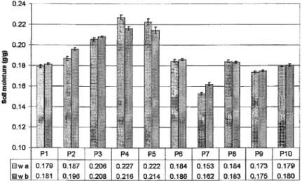
Figure 7: Mean gravimetric moisture contents (wa: 0-15 cm/wb: 15-30 cm) and corresponding standard errors for the 10 test plots.
Figure 8: Dry bulk densities for the 10 test plots.
Soil sampling and analysis: variable soil characteristics.
Soil gravimetric water content (w) was measured for each plot on soil cores collected in the 0-30 cm layer. Ten cores were taken in each plot and divided in two sub-layers (Figure 7) (wa: 0-15 cm/wb: 15-30 cm).
Significant differences in soil moisture between the test plots were observed, whatever the layer considered: 0-15 or 15-30 cm. Points 3-5 were clearly wetter than the other points. This can be explained by the lower elevation of these points, but also by their lower dry bulk density (see below) or higher porosity. The pF curves given above had revealed the ability of this zone to retain water. Conversely, point 7 had the lowest soil moisture. This was also in accordance with the AWC values.
Soil dry bulk density (γd) was measured using undisturbed soil cores as a soil property which is relevant to the
process of compaction. Values ranged from 14.5 to 16.9 kN/m3 (Figure 8). Low values were observed in the
zone corresponding to the old meadow including points 3-6. Especially, the lowest values of γd were obtained at
points 3 and 4 and the highest value was obtained at point 7.
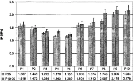
Ten penetrometry profiles (0-80 cm) were recorded in each test plot along the sensor's track and then averaged. The mean cone index in the first 25 cm was computed (IP25). It gave a quick indication of the average resistance of the soil's upper layer. Another parameter was computed (IP10-20). which was the mean cone index between 10
and 20 cm depth, in order to have a comparison basis with other soil parameters measured on soil cores collected at the corresponding depth (Figure 9).
It was observed that points 3-5 showed low cone index values. This is in agreement with the preceding observations: soil at this location showed lower dry bulk densities and higher water content. These elements indicated a better soil structure: meadow, with its deep and strong root system, contributed to develop a good structure in the surface layers. The effect of this structure could still be observed, since this zone was not cultivated so intensively as the rest of the field.
The moisture tension for each plot can be calculated from the curves shown in Figure 6, knowing the water content of the undisturbed cores (Table 1). Two plots are to be noted for exhibiting a moisture tension that was distinctly higher than that of the other plots: point 7 (s = 80.3 kPa) and point 1 (s = 40.1 kPa). This relates to the unconfined compression test results presented below.
Figure 9: Mean cone index values and corresponding standard errors for the 10 test plots.
Unconfined compression tests were performed on undisturbed soil cores. Soil strength σc values ranged from 85
to 185 kPa and deformations at failure εr ranged from 5.5% to 11.3%. Plots 1 and 7 show the highest
compressive resistance. An explanation of this can be found in their high moisture tension values. As well established now (Alonso et al., 1990; Fredlund et al., 1978; Verbrugge and Fleureau, 2002), the shear resistance of the soil increase with moisture tension.
Due to the long duration of this procedure, only a few triaxial tests were performed. They revealed that plots 7-10 could be over-consolidated at low stress levels. Indeed, at low confining pressure (σ3 = 50 kPa), the triaxial
testing curves of some samples exhibited an over-consolidated behaviour.
Synthesis of the experimental plots characteristics.
On basis of the reference tests, three zones could be distinguished. The first one consists of plots 3-6 which presented low dry bulk density, high water content and low cone index values. In the second zone, one finds plots 8-10 which are characterised by low clay content, low plasticity and high cone index values. Plots 1 and 7 form another category, especially due to high suction and high soil strength.
Soil strength mapping
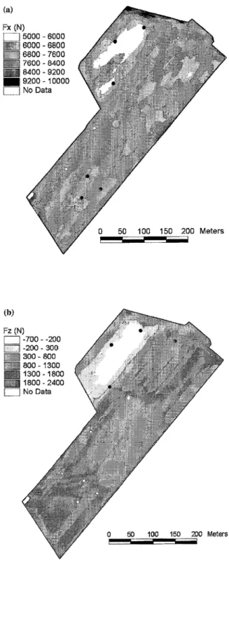
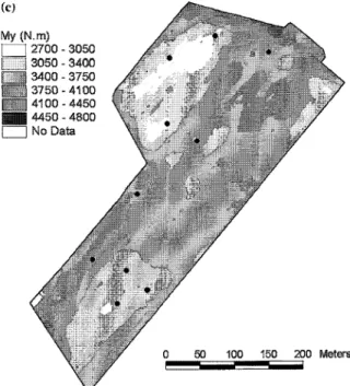
On the basis of the soil strength measurements (1 value per second, total number of points: 9294), values of Fx, Fz and My were interpolated to create continuous maps (Figure 10). Fx and My measurements were highly
correlated (r = 0.93). As a consequence, Fx and Mv maps showed similar patterns. This correlation was due to the
marked predominance of Fx over Fz in the moment because of its higher value and higher lever arm.
Nevertheless, My signal is not completely redundant since it integrates the depth variation of the cutting force
application point.
The variability of the field, mainly due to the differences in texture and in cultivation history, was highlighted. Each map showed a zone located in the old meadow zone and surrounding points 3-5 where the sensor signals were low. In this zone, which was wet and not very compacted, the resistance to soil cutting was relatively small (Figure 10), as well as penetration resistance was low (Figure 9). On the other hand, the Fx and My maps
indicated a zone surrounding points 8-10 with values smaller than in the centre of the field. In contrast to the old meadow, the mean cone index values were high in this zone, resulting from high bulk densities and low moisture content. The origin of this phenomena probably comes from the low clay content which reduces the soil
cohesion and diminishes the failure force encountered by the blade moving in the soil. The third zone around plots 1 and 7 and identified above was not clearly determined by the soil strength sensor. In the eastern zone, containing no reference plots, it was impossible to explain the force fluctuations on a physical basis.
In the old meadow zone, which was known to be more moist, Fz values are positive (directed downwards). This
validates the assumption made by Sirjacobs et al. (2002): the vertical reaction Fz of the soil on the blade is as
much intense and directed upwards as the soil is dry. Indeed, after failure, some soil is forced in an ascending movement in front of the blade and it may be assumed that an increasing moisture reduces the friction forces on the blade. On the other hand, when the soil is moist, it moves laterally, and the blade carries the soil's weight because of its rake angle, which induces a downward vertical reaction. The Fz map showed another area in the
field, where the vertical force was quite high and directed upwards. Unfortunately, there was no reference measurement performed at this location and so, it was impossible to analyse in a more fundamental way this behaviour.
Statistical analysis
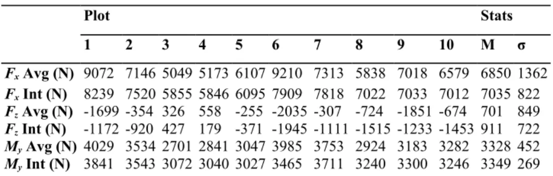
Calculation of forces values within test plots.
The values of Fx, Fz and My within the 10 test plots could be defined in two ways: by taking the average value of
the forces measured during the time the tractor went through each plot, or by interpolating the values of the forces at the centre point of each plot. The second method allowed us to take into account lateral variation of the measurements, which, in some cases, can be important. Both methods are easy to use in the framework of a GIS (Geographic Information System) since positions of the measurement points and of the test plots are precisely known and since the different information layers can be superimposed. ArcView tools were used to extract either the measurement points set for each plot or the corresponding interpolated values. Table 2 shows averaged and interpolated values of measured forces.
(m) and standard deviations (σ) Plot Stats 1 2 3 4 5 6 7 8 9 10 M σ Fx Avg (N) 9072 7146 5049 5173 6107 9210 7313 5838 7018 6579 6850 1362 Fx Int (N) 8239 7520 5855 5846 6095 7909 7818 7022 7033 7012 7035 822 Fz Avg (N) -1699 -354 326 558 -255 -2035 -307 -724 -1851 -674 701 849 Fz Int (N) -1172 -920 427 179 -371 -1945 -1111 -1515 -1233 -1453 911 722 My Avg (N) 4029 3534 2701 2841 3047 3985 3753 2924 3183 3282 3328 452 My Int (N) 3841 3543 3072 3040 3027 3465 3711 3240 3300 3246 3349 269
Correlation analysis: complete data set.
Statistical analysis was performed in order to find any correlation between the signals obtained from the sensor and the reference parameters measured either in situ or in the laboratory.
First exploration of the data was done by means of Pearson's matrix of correlation coefficients. It revealed some significant correlations between soil strength and reference measurements (see Table 3).
Correlation coefficients established on the basis of the interpolated values of measured soil strength showed higher values than those computed on the basis of averaged measurements. Averaged values are representative of the soil resistance along the transects but do not take the lateral variation into account. On the other hand, the reference measurements in each plot were taken close to the transect but not on it and are thus representative of the soil's state within the test plots (which are 5 m wide). This explains why we observed better correlations with the soil's physical parameters using interpolated values, which are influenced by the lateral variations of measurements.
Table 3: Correlation coefficients r between Fx, Fz, My and some of the reference parameters for plots 1-10. Values in brackets are not significant (P > 0.05)
Fx Avg Fz Avg My Avg Fx Int Fx Int My Int
Wab (-0.56) (0.57) (-0.60) -0.79 0.73 -0.74
γd (0.53) (-0.38) 0.65 0.78 (-0.58) 0.81
IP25 (0.34) -0.64 (0.26) (0.50) -0.75 (0.31)
Ic 0.75 (-0.53) 0.80 0.89 (-0.58) 0.89
AWC (-0.53) (0.15) (-0.69) -0.67 (0.17) -0.86
Even though some of the correlation coefficients were quite high, e.g. between interpolated Fx values and
consistency index or between interpolated My values and AWC, the correlations with mean cone index and water
content were markedly inferior to the ones obtained by Sirjacobs et al. (2002). However, these authors only used part of the data and put some particular points aside. They proposed the hypothesis that the state of
over-consolidation observed in some of the plots could modify the soil failure pattern and the stresses exerted on the blade. In this case, the relationships existing between the sensor signals and the physical properties of a normally consolidated soil are probably not valid anymore. Based on the same line of argument, we also made a restricted data set, and computed new correlation coefficients.
Correlation analysis: restricted data set.
Analysis of uniaxial compression tests results showed that plots 7-10 might be over-consolidated. Some confirmation of this was found in the results of the triaxial tests. Moreover, these points present marked
differences with the others: plot 7 because of its high bulk density, moisture tension and clay content and plots 8-10 because of their high cone index values.
A second matrix of correlation coefficients was computed only with values measured in plots 1-6, which are normally consolidated. As expected, r values appreciably increased, mainly for soil moisture content and mean cone index value. Table 4 presents values of the correlation coefficients between forces and other measured physical parameters.
Significant correlations appeared between interpolated Fx values and soil moisture, soil bulk density and cone
index. This last correlation is the consequence of the two others since cone index is known to be a function of soil moisture content and soil dry bulk density. These correlation coefficients tend to prove the sensitivity of the sensor to variations in soil's physical properties. Logically, the more the soil is dense, higher the measured forces are. Likewise, the more the soil is moist, lower the forces are.
Table 4: Correlation coefficients r between Fx, Fz, Mr and some of the reference parameters for plots 1-6. Values in brackets are not significant (P > 0.05)
Fx Avg Fz Avg My AVg Fx Int Fz Int My Int
Wab -0.89 0.85 -0.90 -0.95 (0.80) -0.93
γd (0.70) (-0.59) (0.76) 0.82 (-0.61) 0.88
IP25 0.92 -0.89 0.92 0.95 -0.86 0.89
IC (0.78) (-0.69) 0.83 0.90 (-0.76) 0.89
AWC (-0.63) (0.48) (-0.70) (-0.78) (0.47) -0.91
High correlations were also found between interpolated Fx and consistency index and between interpolated My
and AWC, but similar r values were already found on the basis of the complete data set (10 points). Comparing the above mentioned correlations to those established by Sirjacobs et al. (2002) showed their consistency. Linking IP25 to Fx and My, as it was done in the previous study, would have led to a r2 value
between observed and predicted values of 85.2%, as compared with 80.7% for the previous study. On the other hand, the coefficient of determination between Fz and gravimetric water content was 71.5% instead of 77.9% in the previous experiment. In this study, however, Fx appeared as a better indicator than Fz for soil moisture
content.
Regression analysis.
Even though some significant linear relationships can be defined between measured forces and soil parameters, these are only relevant for certain parts of the field. In the context of precision agriculture, it is obviously much more interesting to generalise such relations to the entire field surface. So, we computed multi-linear
relationships linking one soil parameter to the three signals measured by the dynamometric sensor.
We found the following relationships linking the interpolated values of soil strength to three useful parameters:
These three parameters can also be predicted by means of the plot-averaged values of the measured forces. The coefficients of multiple determination obtained are then respectively, 90.0%, 87.6% and 71.1%.
The multi-linear relationships linking forces to soil parameters allow to go further with the use of these data: it is possible to extrapolate new prediction maps for those soil parameters. We combined the Fx, Fz and My maps, in
accordance with equations above mentioned, and obtained predicted maps for wab, IP10 20 and AWC (see Figure
11).
In the context of precision agriculture, such maps provide valuable information for field management. The cone index map reflects the soil resistance state and could constitute the basic information layer to perform site-specific tillage operations, before seedbed preparation, for example. The AWC map could be relevant information for defining the application map of sowing density.
Classical validation of these maps is, at this time, impossible. Indeed, the whole data set, which is very small (10 points), was used to define the models. As a consequence, the accuracy of the above-mentioned prediction
equations is possibly not very high.
Figure 11: Predicted wab, (a) IP10-20. (b) and AWC (c) maps.
In future experiments, it will be essential to have more reference points within the field, in order to build robust predictions but also to be able to validate the prediction models. In addition, less variables will be measured at each point; only relevant parameters should be focused on, such as soil moisture and penetration resistance profiles. Then, we will be in a position to apply validation methods such as the modified jackknifing method proposed by Bishop and McBratney (2001). The empirical knowledge of the experimental field, however, may give some justification elements.
The soil moisture map clearly shows the limit of the old pasture zone, which is a good "water reservoir" because of the better structure of the soil and also because of its topographical situation (lower elevation). The lowest soil moisture contents are mainly found in the WSW part of the field. This zone was filled up a few years ago and the backfill present underneath the surface soil layer probably acts as a drainage system.
Since the cone index is known to be a function of soil bulk density and water content, the predicted IP10-20 map
reveals the influence of these two parameters. Lowest values are located near points 3-5 which had high water contents and low bulk densities. Highest values are located near point 8-10 which shows low moisture contents and medium bulk densities.
Conclusions
The physical and mechanical properties of a field (10.7 ha) presenting heterogeneity on topographical,
pedological and historical points of view were studied. A set of reference measurements indicated the presence of at least two distinct zones: an old meadow in the lower part of the field, with high porosity and water content and a crest zone characterised by a low clay content and high cone index values.
This study attempted to answer three important questions concerning the soil strength sensor which had previously been tested on a smaller and more homogeneous field and had proved its capability of measuring on-line soil strength variations under field conditions.
(1) Is the sensor suited to distinguish between soil units within the field? Yes. The soil strength maps obtained with the dynamometric sensor coupled with a DGPS confirms the existence of the two zones revealed through the reference measurements. Moreover, these maps may be considered as relevant information layers in the context of precision agriculture: combined with other maps (for example conductivity, plant reflectance maps, etc.) they will help to better understand the factors responsible for final yield.
(2) Is it possible to correlate the measured data to soil physical and mechanical properties? Yes. From both studies, it appears that relationships exist as long as no over-consolidation of the soil occurs. In these particular conditions, soil properties such as cone index and moisture content showed significant correlation with measured draft force. To improve the accuracy of these relationships, numerous reference measurements are needed: their spatial frequency has to be as high as the soil variability. On the other hand, it was possible to establish
prediction equations for three soil properties (namely soil moisture content, cone index and AWC),
independently of the soil's consolidation state, using the three measured force components. Unfortunately, no validation was possible at this time.
(3) Are these reference properties the same as those determined in the last study? Yes. The relationships established between cone index, soil moisture and measured signals have a similar form to those established in the previous study, with comparable coefficients of determination. In this latter study, other soil properties such as consistency index, bulk density and AWC were also significantly correlated to the sensor's signals.
Acknowledgments
The Belgian Ministry of Small Trade and Agriculture is gratefully acknowledged for its financial support to this research.
References
Adamchuk, V. I., Morgan, M. T. and Sumali, H. 2001. Application of a strain gauge array to estimate soil mechanical impedance on-the-go. Transactions of the ASAE 44(6), 1377-1383.
Alonso, E. E., Gens, A. and Josa, A. 1990. A constitutive model for partially saturated soils. Géotechnique 40(3), 405-430.
Andrade, P., Rosa, U., Upadhyaya, S. K., Jenkins, B., Aguera, J. and Josiah, M. 2001. Soil profile force measurements using an instrumented tine. Presented at the 2001 ASAE Annual International Meeting, Paper No 01-1060. ASAE, St. Joseph, MI, USA.
Bishop, T. F. A. and McBratney, A. B. 2001. A comparison of prediction methods for the creation of field-extent soil property maps. Geoderma 103, 149-160.
Clark, R. L. 1999. Soil strength variability within fields. In: Precision Agriculture '99: Papers Presented at the 2nd European Conference on Precision Agriculture, edited by J. V. Stafford (Sheffield Academic Press, Sheffield, UK), pp. 201-210.
Fredlund, D. G., Morgenstern, R. R. and Widger, R. A. 1978. The shear strength of unsaturated soils. Canadian Geotechnical Journal 15, 313-321.
Glancey, J. L., Upadhyaya S. K., Chancellor, W.J. and Rumsey, J. W. 1996. Prediction of agricultural implement draft using an instrumented analog tillage tool. Soil and Tillage Research 37, 47-65.
Godwin, R. J. 1975. An extended octagonal ring transducer for use in tillage studies. Journal of Agricultural Engineering Research 20(4), 345-352.
Guerif, J. 1994. Effects of compaction on soil strength parameters. In: Soil Compaction in Crop Production, edited by B. D. Soane and C. Van Ouwerkerk (Elsevier Science Publishers, Amsterdam, Netherlands), pp. 191-214.
Lui, W., Upadhyaya, S. K., Kataoka, T. and Shibusawa, S. 1996. Development of a texture/soil compaction sensor. In: Proceedings of the Third International Conference on Precision Agriculture. Edited by P. C. Robert, R. H. Rust and W. E. Larsen (ASA-CSSA-SSSA, Madison, WI, USA) pp. 617-630.
Pécrot, A. 1957. Carte des sols de la Belgique et texte explicatif de la planchette de Gembloux (130E). Centre de cartographie des sols. IRSIA. Belgium.
Sirjacobs, D., Hanquet, B., Lebeau, F. and Destain, M. F. 2002. On-line soil mechanical resistance mapping and correlation with soil physical properties for precision agriculture. Soil and Tillage Research 64, 231-242.
Stafford, J. V. 2000. Implementing precision agriculture in the 21st century. Journal of Agricultural Engineering Research 76(3), 267-275.
Upadhyaya, S. K., Chancellor, W. J., Perumpral, J. V., Schafer, R. L. Gill, W. R. and Vandenberg, G. E. 1994. Advances in Soil Dynamics. Vol. 1. ASAE Monograph Number 12 (American Society of Agricultural Engineers, St. Joseph, MI, USA).
Verbrugge, J. C. and Fleureau, J. M. 2002. Bases expérimentales du comportement des sols non saturés. In: Mécanique des sols non saturés, under the supervision of O. Coussy and J. M. Fleureau (Hermès Sciences, Paris, France), pp. 69-112.