A comparison of blade tip timing data analysis
methods
I B Carrington, J R Wright, J E Cooper and G Dimitriadis¤
Dynamics and Aeroelasticity Research Group, School of Engineering, The University of Manchester, UK
Abstract: The experimental determination of the vibration characteristics of rotating engine blades is very important for fatigue failure considerations. One of the most promising techniques for measuring the frequency of blade vibrations is blade tip timing. In this paper, three vibration analysis methods were specifically formulated and applied to the tip timing problem for the first time, using data obtained from a simple mathematical blade tip timing simulation. The results from the methods were compared statistically in order to determine which of the techniques is more suitable. One of the methods, the global autoregressive instrumental variables approach, produced satisfactory results at realistic noise levels. However, all of the techniques produced biased results under certain circumstances.
Keywords: blade tip timing, non-intrusive stress measurement system, vibration analysis, turbomachinery, bladed assemblies, autoregressive methods
NOTATION
a1, a2 autoregressive parameters ^
A amplitude of sine term
An amplitude of cosine term with phase lag
B number of blades
^
B amplitude of cosine term c1, . . ., cB blade damping coefficients
c12, . . ., cB1 interblade coupling damping coefficients
C damping matrix
D mean (d.c.) term
E engine order
f (t) excitation vector
fi(t) force applied to ith blade
F0i amplitude constant for the ith blade
i blade index
j probe index
k1, . . ., kB blade stiffnesses
k12, . . ., kB1 interblade coupling stiffnesses K stiffness matrix m1, . . ., mB blade masses M mass matrix N number of probes R number of revolutions t time ¢t time increment tj discrete time
x vector of blade displacements ~
x displacement (used in the derivation of autoregressive formulation)
xj vector of discrete blade displacements
úl damping ratio of first mode
jn phase lag
ön natural frequency
ön1 natural frequency of first mode
¿ assembly rotational speed 1 INTRODUCTION
Bladed assemblies such as turbines or compressor stages are subject to several sources of excitation leading to forced vibration responses that may occur at or near a blade’s natural frequencies. Other forms of response can occur under conditions such as flutter. Since structural motion can affect the fatigue life, performance and integrity of an assembly [1], the assembly response levels must be monitored. The measurement of rotating blade response is traditionally performed by means of blade-mounted strain gauges. This approach has a number of disadvantages such as a complex installation procedure, a limited number of gauges and the possibility that the gauges might fail at the high temperatures encountered in turbines [2]. In addition, strain gauges require complicated telemetry or slip ring systems and can interfere with the aerodynamic and mechanical properties of the bladed assembly [3].
Blade tip timing, or non-interference stress measurement system (NSMS), is a non-intrusive, non-contacting alter-native to strain gauges. The technique relies on probes
The MS was received on 25 February 2000 and was accepted after revision for publication on 26 June 2001.
¤Corresponding author: Dynamics and Aeroelasticity Research Group,
School of Engineering, The University of Manchester, Oxford Road, Manchester M13 9PL, UK.
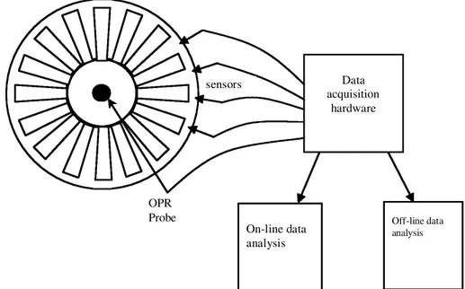
(usually optical) mounted on the engine casing, as shown in Fig. 1, and can measure the motion of every blade. It therefore does not suffer from most of the strain gauge disadvantages. In this work, a maximum of four probes will be considered. The probes measure the time of arrival (ToA) of each blade relative to a once-per-revolution (OPR) or multiple-per-revolution (MPR) probe mounted on the rotor shaft. The difference between the ToA of a vibrating blade and its computed ToA had it not been vibrating provides the raw data from which the instanta-neous blade displacement is found. Blade tip timing data acquisition hardware is now in its fourth generation [4]. Nevertheless, tip timing has a number of disadvantages compared with strain gauges. It cannot detect the blade mode shape and can only be used in an environment where optical visibility is good. However, these disadvantages are outweighed by the ease of installation of the tip timing instrumentation.
‘Synchronous’ or ‘engine-ordered’ blade response occurs when a blade’s vibration frequency is an integer multiple of the engine rotation speed. Synchronous vibrations can be caused by mechanical effects, such as residual unbalance of the rotors and non-concentric casings, as well as aerody-namic effects, such as irregular pressure distributions within the airflow due to the engine intake geometry and wakes produced by upstream stators [5]. ‘Asynchronous’ response occurs when the blade response frequency is a non-integer multiple of the assembly rotation speed. This response condition can be caused either by flutter, a rotating stall, or by acoustic resonance [5].
Tip timing data analysis seeks to extract blade frequency, amplitude and phase, and hence to infer root stress, from the raw data for both synchronous and asynchronous behaviour. The analysis of asynchronous data is a relatively
simple problem since a probe measuring the ToA of a given blade will record different points on the blade’s response cycle for each revolution. However, in the synchronous case, a probe measures the same point on a particular blade’s response cycle at each revolution. Consequently, less information is available than in the asynchronous case and the data analysis process is more involved and more sensitive to noise. This paper will concentrate on the synchronous response problem.
The analysis of blade tip timing data can be performed either ‘on line’ or ‘off line’. ‘On-line’ analysis provides near real-time information updated at least once per second, while ‘off-line’ analysis can provide more detailed information on individual blades, interblade excitations and assembly mistuning effects. However, the raw data contain noise caused by sensor type and blade tip speed, width and surface condition. The present work concentrates on off-line analysis.
Overviews of current methods for analysis of synchro-nous blade tip timing data have been presented in references [1] and [5]. These approaches can be grouped into two categories, direct and indirect:
1. Direct methods use data recorded by a number of probes (typically four) over a limited number of revolutions at a nominally constant rotation speed. Such methods usu-ally attempt a least-squares sine fit of the probe data over the chosen number of revolutions. An example of a direct method is the three- and five-probe method outlined in reference [5].
2. Indirect methods require data from one or two probes spanning an entire resonance region (i.e. the rotational speed varies). The assembly rotation speed must be varied in such a way that the frequency of the excitation
Data acquisition hardware On-line data analysis Off-line data analysis sensors OPR Probe
function sweeps a range of frequencies around the natural frequency of the assembly. Indirect methods can yield estimates for both the engine order and the response amplitude. However, their accuracy suffers in the presence of strong interblade coupling and blade mistuning. Examples of indirect methods are the Zablotsky and Korostolev technique [5] and the two-parameter plot method [6].
This paper presents three new direct methods for synchronous blade tip timing data analysis:
(a) determinant method (DET); (b) global autoregressive (GAR);
(c) global autoregressive with instrumental variables (GARIV).
The methods were applied to a simple lumped parameter model of a multibladed assembly, which was used to produce blade tip timing data for synchronou s responses. The data obtained from this model were corrupted with white noise of varying signal-to-noise levels. The results obtained from all the methods were compared statistically using Monte Carlo simulations.
2 SIMULATED MODEL
The blade tip timing data analysis methods presented in this work were applied to simulated data obtained from a
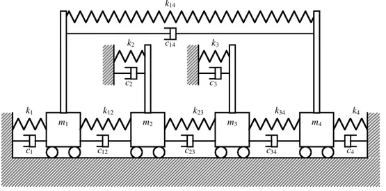
simple mathematical model of the forced synchronous response of a rotating bladed assembly. Sample results were then extracted corresponding to four probe positions that were assumed to be at equal time intervals. Figure 2 shows schematically the basic layout of the model. For illustrative purposes only, four blades are shown in the figure. However, the model could be specified to feature any number of blades. A mass–spring–damper system repre-sents each blade, which is coupled to its two neighbours through two further spring–damper assemblies, so yielding a four-degree-of-freedo m system, one for each blade. In essence, it is assumed that each blade in the assembly has one significant mode, e.g. first banding. Clearly, no rotational dynamics effects (e.g. centrifugal stiffening) are included. The equations of motion were obtained as
Mx ‡ C _x ‡ Kx ˆ f (t) (1)
where x are the degrees of freedom. The normalized mass matrix, M, for a system with B blades is given by
M ˆ 1 0 . . . 0 0 m2=m1 . . . 0 .. . .. . . . . 0 0 0 0 mB=m1 2 6 6 6 4 3 7 7 7 5
the normalized damping matrix, C, is given by
C ˆ 2ú1ön1 c1‡ c12‡ cB1 c1 ¡ c12 c1 0 . . . ¡ c1B c1 ¡cc12 1 c2‡ c12‡ c23 c1 ¡ c23 c1 0 . . . 0 0 ¡cc23 1 c3‡ c23‡ c3B c1 ¡ c3 B c1 . . . 0 .. . .. . .. . .. . .. . .. . ¡cc1 B 1 0 . . . 0 ¡ c3 B c1 cB‡ c3 B‡ cB1 c1 2 6 6 6 6 6 6 6 6 6 6 6 6 6 6 4 3 7 7 7 7 7 7 7 7 7 7 7 7 7 7 5
and the normalized stiffness matrix, K, is given by
K ˆ ö2 n1 k1‡ k12‡ kB1 k1 ¡ k12 k1 0 . . . ¡ k1B k1 ¡kk12 1 k2‡ k12‡ k23 k1 ¡ k23 k1 0 . . . 0 0 ¡kk23 1 k3‡ k23‡ k3 B k1 ¡ k3 B k1 . . . 0 .. . .. . .. . .. . .. . .. . ¡kk1 B 1 0 . . . ¡ k3 B k1 kB‡ k3 B‡ kB1 k1 2 6 6 6 6 6 6 6 6 6 6 6 6 6 6 6 4 3 7 7 7 7 7 7 7 7 7 7 7 7 7 7 7 5
whereö2
n1 ˆ k1=m1 and ú1ˆ c1=(2m1ön1) act as normal-izing factors.
A sinusoidal excitation force of frequency öf was applied to each mass. The force pattern could be chosen to excite any mode of interest and is given by
fi(t) ˆ F0isin E¿t ‡ 2ðEi
B
³ ´
, for i ˆ 0, 1, . . ., B ¡ 1 where fiis the force applied to the ith blade (with units of
acceleration owing to the normalization), F0i is an amplitude constant,¿ is the angular rotation speed of the assembly and E is the engine order, i.e. the integer ratio of the excitation frequency to the assembly rotation speed E ˆ öf=¿.
Steady state conditions were considered so that blade responses were purely sinusoidal. The sensor positions were equally spaced along a time axis to give a constant intersensor time interval,¢t (this will occur approximately if the sensors are equally spaced spatially). Each blade response included a different d.c. offset to simulate constant local gas loading.
Blade positions were incremented in time and blade response displacement values recorded when blade posi-tions matched probe posiposi-tions. The probes could be offset from the 08 phase response position for blade 1. Additive white noise was used to corrupt the response data to simulate the experimental measurement uncertainties.
3 ANALYSIS METHODS
Methods for analysing tip timing data have been developed since 1970. However, given a limited number of probes, there are still no standard approaches that can identify
synchronous response resonance frequencies with adequate certainty [6]. The three methods for tip timing data analysis introduced in this work either are new (DET) or have never been adapted to the tip timing problem before (GAR, GARIV).
The synchronous response blade tip timing problem would be much simpler if the measurements were noise free. However, there are a number of factors associated with the data acquisition procedure that can contribute to significant levels of experimental measurement uncertainty. The methods for the evaluation of the spectral character-istics of the synchronous blade responses presented here were investigated statistically to determine the sensitivity of each technique to noise level.
All the methods assume that the tuned synchronous response at resonance (i.e. öf ˆ ön) for a particular blade is a single frequency sinusoid of the form
x ˆ Ancos(önt ‡ jn) ‡ D (2)
where x is the blade response amplitude, An,önand jnare the response amplitude, relevant natural frequency and phase respectively at engine order E and D is the d.c. blade offset. The identification problem is to determineön, and hence the engine order, amplitude, phase and offset, from the response data obtained when the blade(s) of interest passes the probes.
3.1 Determinant method (DET)
An alternative single-blade expression, equivalent to equa-tion (2) is xjˆ ^Acos(öntj) ‡ ^B sin(öntj) ‡ D (3) m1 m2 m3 m4 k12 k1 k23 k34 k4 k3 k2 c2 c3 c1 c12 c23 c34 c4 k14 c14
where j denotes measurements taken as the blade passes the jth probe.
Equation (3), containing four unknowns, can be ex-panded for j ˆ 1, . . ., 4 to yield enough equations for the parameters ^A, ^B,önand D to be evaluated from measure-ments over one single rotation, assuming that four probes are available. Elimination of ^A, ^B and D yields the following equation: XX34¡ S¡ S34 CC34¡ S¡ S34 ˆ 0 (4) where Xjˆ xxj¡ x1 2¡ x1
Cjˆcos(cos(öntj) ¡ cos(önt1)
önt2) ¡ cos(önt1)
Sjˆsin(sin(öntj) ¡ sin(önt1)
önt2) ¡ sin(önt1) for j ˆ 3, 4.
By evaluating the determinant of equation (4) for differ-ent candidate values ofön, the value that satisfies equation (4) exactly can be found in the absence of noise. When noise is present, equation (4) can only be satisfied approximately and it is assumed that the closest result yields the true frequency. For a synchronous resonance, önˆ E¿, where ¿ is the assembly’s angular velocity and
Eis the engine order. Hence the value of E for which the determinant is closest to zero is taken as the resonance engine order in the presence of noise. The other unknown parameters, ^A, ^B and D, can be obtained using back substitution.
Candidate values of ön are those which correspond to synchronous engine-ordered responses, i.e. integer multi-ples of the rotational frequency¿, subject to the frequency limitation imposed by
ömaxˆ32ð
¢t (5)
where 3¢t is the difference in ToA between the first and fourth probes.
Equation (5) defines a maximum frequency below which all four data points will appear only once over one sine wave cycle. Solutions to equation (4) may exist aboveömax but, in this study, only synchronous response frequencies up toömaxare considered.
The DET approach can only be applied to data from one blade, obtained over a single revolution of the assembly. In a typical tip timing test, data from all blades will be available, recorded over a number of revolutions. Hence, the DET frequency (or engine order) results from each
blade and each revolution can be averaged in order to provide a single, more reliable, frequency estimate.
3.2 Autoregressive methods (AR)
In order to set up an AR [7] formulation of the blade tip timing data analysis problem, the ordinary differential equation (ODE)
~x ‡ ö2
n~x ˆ 0 (6)
whose solution is given by ~x ˆ Ancos(önt‡ jn) ‡ D can be used. The ODE of equation (6) can be approximately discretized by writing the two possible second-order Taylor expansions for ~x around time instance tj:
~ x(tj‡ ¢t) ˆ ~x(tj) ‡ ¢t _~x tj ‡¢t 2 2 ~x tj and, substituting¢t ˆ ¡¢t, ~ x(tj¡ ¢t) ˆ ~x(tj) ¡ ¢t _~x tj ‡¢t 2 2 ~x tj
Adding the two Taylor expansions, an expression for the second derivative of ~x at time tjcan be obtained:
~xjˆ ~xj‡1¡ 2~x¢t2j‡ ~xj¡1 (7)
where ~xjis simplified notation for ~x(tj) and ~xj§1 stands for
~
x(tj§ ¢t). Notice that equation (7) only holds in the case
where the time steps between any three consecutive, discrete data points are constant. Hence, by using this approach to analyse tip timing data, it is assumed that the differences in ¢t due to the blade vibrations are small enough not to invalidate equation (7). Using expression (7), the second-order ODE of equation (6) can be rewritten as ~ xj‡1¡ 2~xj‡ ~xj¡1 ¢t2 ‡ ö2nx~jˆ 0 or ~ xj‡1‡ (¢t2ö2n¡ 2)~xj‡ ~xj¡1ˆ 0 (8)
Finally, by delaying equation (8) by ¢t, writing a1ˆ ¢t2ö2n¡ 2 and introducing a d.c. term by substituting ~
xjˆ xj‡ D, the AR formulation of the
single-degree-of-freedom blade tip timing data analysis problem becomes xj‡ a1xj¡1‡ xj¡2ˆ D(2 ‡ a1) (9) Equation (9) is of the form xjˆ ¡a1xj¡1¡ a2xj¡2,
term added. The simplest way of solving equation (9) using a data sequence is to expand it columnwise as
x3‡ x1 x4‡ x2 .. . xN ‡ xN¡2 2 6 6 6 4 3 7 7 7 5ˆ x2 1 x3 1 .. . .. . xN¡1 1 2 6 6 6 4 3 7 7 7 5 ¡a1 D(2 ‡ a1) µ ¶ (10)
where N is the data record length. Equation (10) is of the form
b ˆ Xa (11)
and can be solved for a in a least-squares sense:
a ˆ (XTX)¡1XTb (12)
Hence, the simplest AR solution for the tip timing problem can be obtained by solving equations (10) for a single blade and a single revolution, such that N is the number of tip timing probes.
The problem with this simple approach is that, if the data points x1, . . ., xNcontain experimental errors, the estimates
for the AR parameters a1 and the offset D will be biased [8]. In order to counteract the bias, two more advanced AR approaches were considered for this study.
3.2.1 Global AR (GAR)
This approach is essentially the simple least-squares scheme outlined in equation (10), the main difference being that the equations for all blades and all revolutions are solved simultaneously to yield a single, global, value of a1 (and, hence, the frequency) and a value of D for each blade. The global system of equations to be solved is of the form
where B is the total number of blades, N is the number of probes and R is the number of revolutions. For the GAR approach, equation (13) was solved using simple least squares. Clearly, the assumption here is that all blades exhibit the same frequency of vibration, although not the same offset and amplitude.
3.2.2 Global AR with instrumental variables (GARIV) An instrumental variables (IV) approach [8, 9] was also used to solve the global AR equations (13). The equations are first pre-multiplied by a suitable IV matrix composed of delayed observations giving
Xib ˆ XiXa
The least-squares solution to this new problem is
a ˆ (XT
iX)¡1XTib (14)
The chosen delay was in the region of 10 per cent of the total number of revolutions. This approach is classified in the literature as a ‘noise allowing’ parameter estimation technique. It aims to reduce the bias in the estimates by using the delayed observations in order to avoid the correlation terms in the XT
iX matrix that give rise to bias.
Other, iterative, IV approaches could also be employed.
4 THE EFFECT OF NOISE ON LEAST-SQUARES ESTIMATES
When there is noise in the data, the least-squares estimates will contain two types of error:
1. Bias is where the estimates are incorrect even if an 1x 1,1‡1x1,3 .. . 1x 1, N ¡2‡1x1, N .. . 1x B,1‡1xB,3 .. . 1x B,N ¡2‡1xB,N .. . Rx 1,1‡Rx1,3 .. . Rx 1, N ¡2‡Rx1, N .. . Rx B,1‡RxB,3 .. . Rx B,N ¡2‡RxB,N 2 6 6 6 6 6 6 6 6 6 6 6 6 6 6 6 6 6 6 6 6 6 6 6 6 6 6 6 6 6 6 6 6 4 3 7 7 7 7 7 7 7 7 7 7 7 7 7 7 7 7 7 7 7 7 7 7 7 7 7 7 7 7 7 7 7 7 5 ˆ 1x 1,2 1 0 . . . 0 .. . .. . .. . .. . .. . 1x 1,N¡1 1 0 . . . 0 .. . .. . .. . .. . .. . 1x B,2 0 0 . . . 1 .. . .. . .. . .. . .. . 1x B,N ¡1 0 0 . . . 1 .. . ... .. . .. . .. . Rx 1,2 1 0 . . . 0 .. . .. . .. . .. . .. . Rx 1,N¡1 1 0 . . . 0 .. . .. . .. . .. . .. . Rx B,2 0 0 . . . 1 .. . .. . .. . .. . .. . Rx B,N¡1 0 0 . . . 1 2 6 6 6 6 6 6 6 6 6 6 6 6 6 6 6 6 6 6 6 6 6 6 6 6 6 6 6 6 6 6 6 6 4 3 7 7 7 7 7 7 7 7 7 7 7 7 7 7 7 7 7 7 7 7 7 7 7 7 7 7 7 7 7 7 7 7 5 ¡a1 D1(2 ‡ a1) .. . DB(2 ‡ a1) 2 6 6 6 4 3 7 7 7 5 (13) First revolution First blade 8 > < > : 8 > > > > > > > > > > > > > < > > > > > > > > > > > > > : Bth blade 8 > > > > < > > > > : Rth revolution 8 > > > > > > > > > > > > > < > > > > > > > > > > > > > :
infinite amount of data is included. It is caused by a summated squared noise term in the XT
iX matrix that
does not tend to zero but increases with increasing noise levels. This is an effect of the autoregressive model that is used.
2. Scatter, where there is a range of estimates spread about the mean value, is caused by random variations in the data.
The best method will exhibit the lowest bias and, preferably, lowest scatter.
5 STATISTICAL ANALYSIS AND COMPARISON OF METHODS
5.1 Monte Carlo simulations
Comparison of the methods was performed using Monte Carlo simulations. A white noise generator was used to create 100 distinct noise sequences with which to corrupt the data obtained from the tip timing simulator. Each test was repeated using all the white noise sequences for each method. The mean and variance of the recovered engine orders were computed, from which 95 per cent confidence intervals were obtained.
The objective of the tests was to assess the accuracy of each method under a variety of conditions. For all the tests, it was assumed that all the blades were identical (perfectly tuned), i.e.
k1 ˆ k2ˆ ¢ ¢ ¢ ˆ kB
m1ˆ m2ˆ ¢ ¢ ¢ ˆ mB
c1ˆ c2ˆ ¢ ¢ ¢ ˆ cB
and that all the coupling ratios were also identical and equal to 10 per cent, i.e.
k12=k1ˆ k23=k1 ˆ ¢ ¢ ¢ ˆ 0:1
c12=c1ˆ c23=c1ˆ ¢ ¢ ¢ ˆ 0:1
The excitation frequency for all the tests was chosen to be equal to the basic natural frequency of the system, i.e. öf ˆ ön1ˆpk1=m1, in order to induce a resonant response in the first mode. The main test parameters were as follows:
(a) engine order value (E );
(b) probe spacing on the resonance (PSR); (c) probe 1 offset on the resonance (P1off); (d) number of blades (B);
(e) number of revolutions (R); (f) noise-to-signal ratio (NSR).
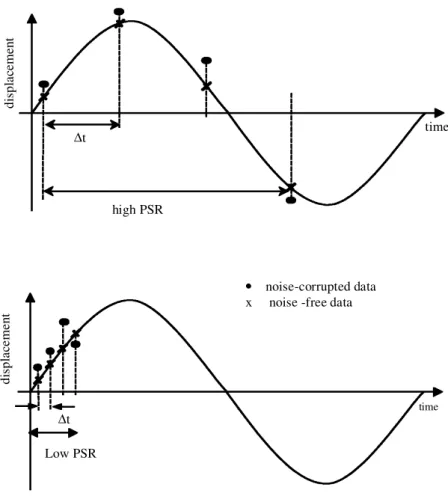
PSR refers to the time difference between the first and fourth probe outputs as a percentage of the blade resonance
response period, as shown in Fig. 3. The top plot in Fig. 3 shows a very high PSR (¹ 65 per cent); the bottom plot shows a low PSR (¹ 15 per cent). Clearly, curve fitting a sine wave through noisy data with a low PSR will be more prone to error than for a high PSR. P1off describes the amount by which the first probe is offset from the start of the blade response cycle, i.e. the position at which the response of blade 1 has 08 phase.
Six test cases are presented to demonstrate the effects of each parameter on the quality of the identification of each method. These are shown in Table 1.
Test 1 was specifically chosen to be a very difficult case to analyse. Hence, the other tests were used to investigate whether specific changes in the parameters improve the quality of identification.
5.2 Results
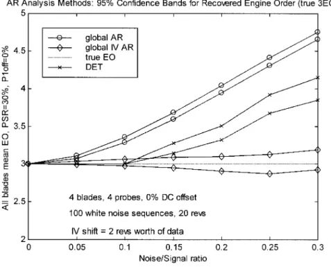
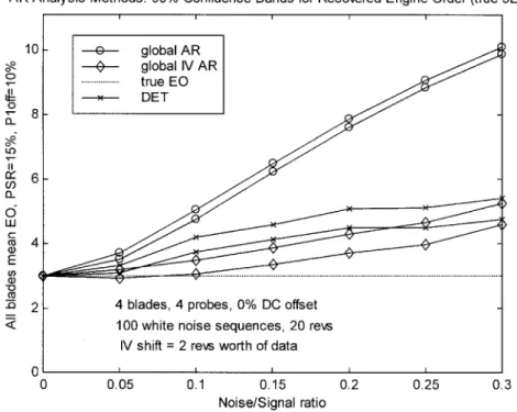
All the methods delivered exact answers in the absence of noise (i.e. when the noise level is zero). The results obtained from the Monte Carlo simulations are reproduced in Figs 4 to 9. The figures plot the 95% confidence intervals for the value of the engine order recovered by each method against NSR. NSR is defined as the ratio of the r.m.s. value of the noise to the r.m.s. value of the ‘clean’ probe displacements. Note that, even though the engine order resulting from each test was an integer (i.e. the estimated engine order was rounded to the nearest integer value), the confidence bounds plotted in the figures are real numbers.
The analysis of the test cases yields the following main conclusions:
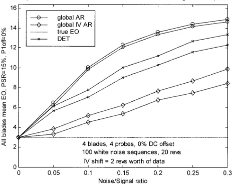
1. As expected, test 1 was a very difficult case. As shown in Fig. 4, all the methods produced biased results, even at low NSR values.
2. Increasing the number of blades from 4 to 12 produced a dramatic increase in the accuracy of the GARIV and DET methods. Figure 5 shows that GARIV results for test 2 were unbiased up to a noise level of 17.5 per cent while DET results were unbiased up to 5 per cent. The predictions of the GAR method, even though much closer to the true values than in test 1, were still biased. This increase in the quality of the results was due to the increase in the number of data points and the variety of response amplitudes used in the estimation procedures. The larger data samples alleviated to a certain extent the effect of the noise.
3. Increasing the number of revolutions over which data were used for the identification process also improved the results. However, as shown in Fig. 6, the improve-ment was not as dramatic as in the case of test 2 (Fig. 5). GARIV results were unbiased up to NSR ˆ 8 per cent but both DET and GAR predictions were still biased. The increase in quality was caused by the increase in the volume of data used in the estimation procedures.
4. Increasing the PSR value to 30 per cent produced the most dramatic improvement in the quality of the identification. Figure 7 shows that GARIV results were unbiased throughout the noise range investigated. In addition, the engine order data obtained using DET were also unbiased up to NSR ˆ 10 per cent. Finally, even though GAR results were still biased up to NSR ˆ 10 per cent, the GAR-recovered engine orders were below 3.5 which means that on average, when rounded, they would deliver the correct value. As already discussed, curve fits of higher PSR data are generally much more accurate than those of low PSR data.
5. Increasing the probe 1 offset to 10 per cent moved the data towards the peak of the response sine wave. Since the function is more curved around the peak, the data were more characteristic of a sine wave. Hence, the accuracy of the recovered engine orders improved, as
can be seen in Fig. 8. GARIV results were unbiased up to 7.5 per cent NSR. The engine orders recovered by the other two methods were less biased than in the test 1 case.
6. Increasing the engine order of the tip timing data had no visible effect on the accuracy of the identification. Figure 9, which shows the results for test 6, is a scaled version of Fig. 1. This is not surprising since the effect of the engine order is to scale the response frequency up or down while keeping the PSR constant.
The behaviour of individual methods can be summarized as follows:
1. The determinant method exhibited high levels of bias in general. However, in the case of higher values of probe spacing on the resonance (see Fig. 7), the approach became extremely accurate at noise levels up to 10 per cent NSR. This increased accuracy occurs because, at higher PSR, the determinant method permits only one or two frequencies to be possible solutions. Hence, a correct result for engine order is more likely.
2. The GAR method always returned the most highly biased results and provided the least accurate estimates, as can be seen in all the figures. However, it exhibited low scatter and was computationally more efficient than the determinant method.
3. GARIV gave the least biased results of all three
time di sp la ce m en t Dt time di sp la ce m en t noise-corrupted data x noise -free data high PSR
Low PSR Dt
Fig. 3 High and low PSR values Table 1 Test cases
PSR P1off B Probes R True E
Test 1 15% 0% 4 4 20 3 Test 2 15% 0% 12 4 20 3 Test 3 15% 0% 4 4 100 3 Test 4 30% 0% 4 4 20 3 Test 5 15% 10% 4 4 20 3 Test 6 15% 0% 4 4 20 8
methods. For tests 2 to 5, GARIV yielded unbiased results up to various values of NSR despite the fact that the other methods generally gave biased results at all noise levels. The cost of reducing the bias is clearly seen in all figures to be an increase in scatter, as compared
with the GAR scatter values.
Consequently, GARIV appears to be a very promising approach for analysing tip timing data. However, it should be mentioned that approach sometimes fails to recover an Fig. 4 Test 1 results: benchmark (EO, engine order)
engine order. The a1 term in equation (9), developed from an approximate treatment, is defined as a1ˆ (¢t2ö2n¡ 2). By performing the transformation from continuous to discrete time, it can be shown that a1 ˆ ¡2 cos(ön¢t). Hence, the engine order is given by
E ˆ¿ ¢t1 cos¡1 ¡a1 2
³ ´
(15) As a consequence, if the identified value of a1 is such that ja1=2j . 1, it is impossible to recover a real engine order.
Fig. 6 Test 3 results: effect of increased number of revolutions
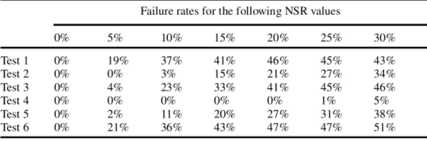
This failure can occur when using the GARIV method, especially at high NSR values. Table 2 shows the percent-age of failure of the technique for test cases 1 to 6.
Table 2 shows that the worst failure rates occur at cases
where the GARIV predictions are highly biased anyway and, consequently, do not greatly affect the ability of the approach to identify tip timing data. It should also be noted that, in practice, the NSR values rarely exceed 10 per cent. Fig. 8 Test 5 results: effect of increased P1off
6 CONCLUSIONS
Three new methods for the analysis of blade tip timing data have been presented and applied to a simple mathematical model of the blade tip timing measurement process. White noise was added to corrupt the data and Monte Carlo simulations were used to investigate the performance of the methods statistically. The object of the comparison was to assess analysis techniques for determining the vibration engine order.
The least biased results were obtained from the GARIV approach. At modestly high values of PSR (30 per cent), GARIV gave unbiased results. However, at low PSR and for certain combinations of parameters, all the methods exhibited biased behaviour. The noise at low PSR was very difficult to resolve because of the small number of probes. Hence, in some cases, a sufficient number of equations could not be obtained to counteract the bias. All the methods appeared to work better in the presence of a high probe 1 offset and a large number of blades and revolutions.
More refined techniques will be explored in future work on the analysis of blade tip timing data.
ACKNOWLEDGEMENTS
The authors would like to thank Rolls–Royce plc and EPSRC who supported this work under the Engineering Doctorate scheme.
REFERENCES
1 Heath, S., Slater, T., Mansfield, L. and Loftus, P.
Turboma-chinery blade tip measurement techniques. In AGARD Con-ference Proceedings 598 on Advanced Non-Intrusive
Instrumentation for Propulsion Engines, Brussels, Belgium,
1997.
2 Robinson, W. W. and Washburn, R. S. A real time
non-interference stress measurement system (NSMS) for determin-ing aero engine blade stress. In Proceeddetermin-ings of the 37th Symposium of the Instrumentation Society of America, San Diego, California, 1991, pp. 91–103.
3 Heath, S. and Imregun, M. A review of analysis techniques
for blade tip-timing measurements. In International Gas Turbine and Aero Engine Congress and Exhibition, Orlando, Florida, 1997, paper 97-GT-213.
4 Robinson, W. W. Overview of Pratt and Whitney NSMS. In
45th International Instrumentation Symposium, Albuquerque, New Mexico, May 1999.
5 Zielinski, M. and Ziller, G. Optical blade vibration
measure-ment at MTU. In AGARD Conference Proceedings 598 on
Advanced Non-Intrusive Instrumentation for Propulsion
En-gines, Brussels, Belgium, 1997.
6 Heath, S. A new technique for identifying synchronous
resonances using tip-timing. In International Gas Turbine and Aeroengine Congress and Exhibition, Indianapolis, Indiana, 1999, paper 99-GT-402.
7 Astrom, K. J. and Eykhoff, P. System identification—a
survey. Automatica, 1971, 7, 123 –162.
8 Cooper, J. E. Comparison of some time-domain-system
identification techniques using approximate data correlations.
J. Modal Anal., April 1989, 4, 51– 57.
9 James, P. N., Souter, P. and Dixon, D. C. A comparison of
parameter estimation algorithms for discrete systems. Chem.
Engng Sci., 1974, 29, 539 –547.
Table 2 Failure rate of GARIV method Failure rates for the following NSR values
0% 5% 10% 15% 20% 25% 30% Test 1 0% 19% 37% 41% 46% 45% 43% Test 2 0% 0% 3% 15% 21% 27% 34% Test 3 0% 4% 23% 33% 41% 45% 46% Test 4 0% 0% 0% 0% 0% 1% 5% Test 5 0% 2% 11% 20% 27% 31% 38% Test 6 0% 21% 36% 43% 47% 47% 51%