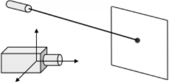
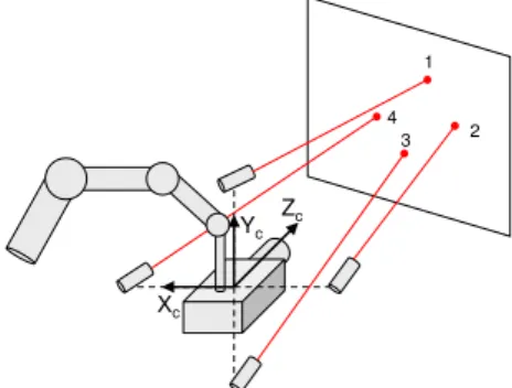
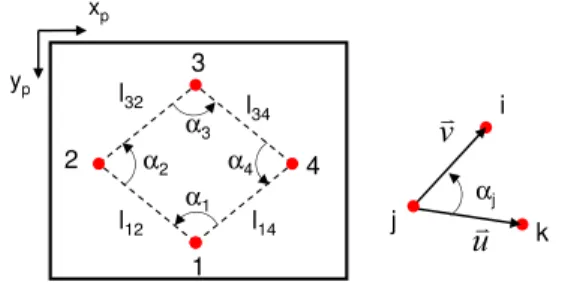
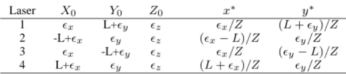
Plane-to-plane positioning from image-based visual servoing and structured light
Texte intégral
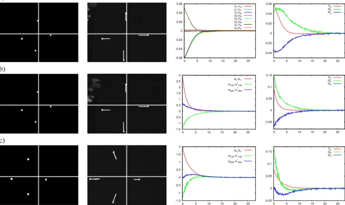
Figure
Documents relatifs
Ces doubles cursus médecine-sciences encouragent la validation d’un Master 2 scientifique avant le 2 e cycle des études médicales, idéalement suivie d’une thèse de sciences
We compared DNA preparation methodologies (DNA extraction directly from either phage lysates or CsCl purified phage particles), and sequencing strategies that utilize either
found recently in the iConnect study that a 1-year decrease in cycling for commuting (not for walking) was associated with a decrease in LTPA [19]. A limitation in previous
The operational semantics that we proposed, is useful for the formalization of refinement relation. In- deed, an operational semantics is concretely given as a guarded
Au-delà de l’échelon local, l’enjeu minier relève d’une politique sectorielle et globale (fiscale, économique, de développement, etc.) qui constitue le cadre général dans
Afin de comprendre comment TFIIA communique avec les activateurs pour stimuler la transcrip- tion, un complexe entre TFIIA, TFIID, Rap1 et l’ADN promoteur a été analysé [8]...
Para maturação muito precoce temos somente o Catucaí 785-15 com média de produtividade de 07 safras de 35,8 Sc/ha e está em destaque entre os 22 melhores genótipos testados
Pour des raisons différentes, ces deux scénarios ne four- nissent pas d’explications satisfaisantes à l’existence des virus géants, ni à la composition de leur génome, en
