Montréal
Série Scientifique
Scientific Series
2001s-56Exact Nonparametric
Two-Sample Homogeneity Tests for
Possibly Discrete Distributions
CIRANO
Le CIRANO est un organisme sans but lucratif constitué en vertu de la Loi des compagnies du Québec. Le financement de son infrastructure et de ses activités de recherche provient des cotisations de ses organisations-membres, d’une subvention d’infrastructure du ministère de la Recherche, de la Science et de la Technologie, de même que des subventions et mandats obtenus par ses équipes de recherche.
CIRANO is a private non-profit organization incorporated under the Québec Companies Act. Its infrastructure and research activities are funded through fees paid by member organizations, an infrastructure grant from the Ministère de la Recherche, de la Science et de la Technologie, and grants and research mandates obtained by its research teams.
Les organisations-partenaires / The Partner Organizations
•École des Hautes Études Commerciales •École Polytechnique
•Université Concordia •Université de Montréal
•Université du Québec à Montréal •Université Laval
•Université McGill
•Ministère des Finances du Québec •MRST
•Alcan inc. •AXA Canada •Banque du Canada
•Banque Laurentienne du Canada •Banque Nationale du Canada •Banque Royale du Canada •Bell Québec
•Bombardier •Bourse de Montréal
•Développement des ressources humaines Canada (DRHC) •Fédération des caisses Desjardins du Québec
•Hydro-Québec •Industrie Canada
•Pratt & Whitney Canada Inc. •Raymond Chabot Grant Thornton •Ville de Montréal
© 2001 Jean-Marie Dufour et Abdeljelil Farhat. Tous droits réservés. All rights reserved. Reproduction partielle permise avec citation du document source, incluant la notice ©.
Short sections may be quoted without explicit permission, if full credit, including © notice, is given to the source.
Ce document est publié dans l’intention de rendre accessibles les résultats préliminaires de la recherche effectuée au CIRANO, afin de susciter des échanges et des suggestions. Les idées et les opinions émises sont sous l’unique responsabilité des auteurs, et ne représentent pas nécessairement les positions du CIRANO ou de ses partenaires.
This paper presents preliminary research carried out at CIRANO and aims at encouraging discussion and comment. The observations and viewpoints expressed are the sole responsibility of the authors. They do not necessarily represent positions of CIRANO or its partners.
Exact Nonparametric Two-Sample Homogeneity Tests for
Possibly Discrete Distribution
*Jean-Marie Dufour
†, Abdeljelil Farhat
‡Résumé / Abstract
Dans ce texte, nous étudions plusieurs tests pour l'egalité de deux
distributions inconnues. Deux de ces tests sont basés sur des fonctions de
distribution empiriques, trois autres sur des estimateurs non-paramétriques de
fonctions de densité, et les trois derniers sur des moments empiriques. Nous
proposons de contrôler la taille des tests (sous des hypothèses non-paramétriques)
en employant des versions permutationnelles de ces tests conjointement avec la
méthode des tests de Monte Carlo ajustée pour tenir compte de la possibilité de
distributions discontinues. Nous proposons aussi une méthode pour combiner
plusieurs de ces tests, le niveau de ces procédures étant aussi contrôlé par la
technique des tests de Monte Carlo, laquelle possède de meilleures propriétés de
puissance que les tests individuels combinés. Finalement, nous montrons dans une
étude de simulation que la technique suggérée contrôle parfaitement la taille des
différents tests considérés et que les nouveaux tests proposés peuvent fournir de
notables améliorations de puissance.
In this paper, we study several tests for the equality of two unknown
distributions. Two are based on empirical distribution functions, three others on
nonparametric probability density estimates, and the last ones on differences
between sample moments. We suggest controlling the size of such tests (under
nonparametric assumptions) by using permutational versions of the tests jointly
with the method of Monte Carlo tests properly adjusted to deal with discrete
distributions. We also propose a combined test procedure, whose level is again
perfectly controlled through the Monte Carlo test technique and has better power
properties than the individual tests which are combined. Finally, in a simulation
experiment, we show that the technique suggested provides perfect control of test
size and that the new tests proposed can yield sizeable power improvements.
*
Corresponding Author: Jean-Marie Dufour, CIRANO, 2020 University Street, 25th floor, Montréal, Qc, Canada H3A 2A5 Tel.: (514) 985-4000 Fax: (514) 985-4039 email: [email protected] The authors thank Serge Tardif for his numerous comments. This work was supported by the Canada Research Chair Program, the Canadian Network of Centres of Excellence [program on Mathematics of Information Technology and Complex Systems (MITACS)], the Canada Council for the Arts (Killam Fellowship), the Natural Sciences and Engineering Research Council of Canada, the Social Sciences and Humanities Research Council of Canada, and the Fonds FCAR (Government of Québec).
Mots Clés :
Méthodes non-paramétriques, problème des deux échantillons, distribution
discrète, distribution discontinue, test d'ajustement, test de Kolmogorov-Smirnov,
estimateur à noyau pour une densité, test exact, test de permutations, test de
Monte Carlo, bootstrap, test combiné, test induit
Keywords:
Nonparametric methods, two-sample problem, discrete distribution, discontinuous
distribution, goodness-of-fit test, Kolmogorov-Smirnov test, Cramér-von Mises,
kernel density estimator, exact test, permutation test, Monte Carlo test, bootstrap,
combined test procedure, induced test
Contents
1. Introduction 1
2. Test statistics 2
3. Exact randomized permutation tests 5
4. Monte Carlo standardized combined tests 7
5. Simulation study 8
6. Conclusion 12
List of Tables
1 Continuous distributions with their means and variances . . . . 9 2 Empirical level and power for MC permutation tests of equality of two distributions 9 3 Some illustrations for empirical level for KS and CM tests of equality of two
con-tinuous distributions . . . . 10 4 Some illustrations for empirical level for KS and CM tests of . . . . 10 5 Empirical level and power for MC permutation tests of equality of two continuous
distributions having same mean and same variance . . . . 13 6 Empirical level and power for MC permutation tests of equality of two continuous
distributions having different means but same variance . . . . 14 7 Empirical level and power for MC permutation tests of equality of two continuous
distributions having same mean but different variances . . . . 15 8 Empirical level and power for MC permutation tests of equality of two continuous
distributions having different means and different variances . . . . 16 9 Empirical level and power for MC permutation tests of equality of two discrete
distributions having same mean but different variances . . . . 17 10 Empirical level and power for MC permutation tests of equality of two discrete
distributions having different means and same variance . . . . 18 11 Empirical level and power for MC permutation tests of equality of two discrete
1.
Introduction
An important problem in statistics consists in testing whether the distributions of two random vari-ables are identical against the alternative that they differ in some way. Specifically, consider two random samples X1, . . . , Xn and Y1, . . . , Ym such that F (x) = P[Xi ≤ x], i = 1, ... , n, and G(x) = P[Yj ≤ x], j = 1, ... , m. We shall not impose here additional restrictions on the form
of the cumulative distribution functions (cdf) F and G, which may be continuous or discrete. The problem consists in testing the null hypothesis
H0: F = G (1.1)
against the alternative
H1 : F 6= G . (1.2)
H0 is a nonparametric hypothesis, so testing H0 requires a distribution-free procedure. Thus, many users who have to make such a confrontation resort to a goodness-of-fit test, usually the two-sample Kolmogorov-Smirnov (KS) test [Smirnov (1939, 1948)] or the Cramér-von Mises (CM ) test [Lehmann (1951), Rosenblatt (1952) and Fisz (1960)]. Other procedures that have been sug-gested include permutation tests based on L1 and L2 distances between kernel-type estimators of the relevant probability density functions (pdf) [Allen (1997)] and tests based on the difference of the means of the two samples considered [Pitman (1937), Dwass (1957), Efron and Tibshirani (1993)]. Except for the last procedure, which is designed to have power against samples that differ through their means, the exact and limiting distributions of the test statistics are not standard, and tables for the exact distributions are only available for a limited number of sample sizes. Thus these tests are usually performed with the help of tables based on asymptotic distributions. This leads to procedures that do not have the targeted size (which can easily be too small or too large) and may have low power.
In this paper, we aim at finding test procedures with two basic features. Namely, the latter should be: (1) truly distribution-free, irrespective of whether the underlying distribution F is dis-crete or continuous, and (2) exact in finite samples (i.e., they must achieve the desired size even for small samples). In this respect, it is important to note that the finite and large sample distribu-tions of usual test statistics are not necessarily distribution-free under H0. In particular, while the KS and CM statistics are distribution-free when the observations are independent and identically
distributed (i.i.d.) with a continuous distribution, this is not anymore the case when they follow a discrete distribution. For the statistics based on kernel-type density estimators, distribution-freeness does not obtain even for i.i.d observations with a continuous distribution. This difficulty can be relaxed by considering a permutational version of these tests which uses the fact that all permuta-tions of the pooled observapermuta-tions are equally likely when the observapermuta-tions are i.i.d with a continuous distributions. The latter property, however, does not hold when the observations follow a discrete distribution. So none of the procedures proposed to date for testing H0 satisfies the double require-ment of yielding a test that is both distribution-free and exact.
Given recent progress in computing power, a way to solve this difficulty consists in using simulation-based methods, such as bootstrapping or Monte Carlo tests. The bootstrap technique
however does not ensure that the level will be fully controlled in finite samples [for further dis-cussion of bootstrapping, see Efron and Tibshirani (1993), Hall (1992), Shao and Tu (1995) and Davison and Hinkley (1997)]. For this reason, we favor Monte Carlo (MC) test methods. MC tests were introduced by Dwass (1957) and Barnard (1963). Further discussions and extensions are also available in Birnbaum (1974), Foutz (1980), Jöckel (1986), Dufour (1995), Kiviet and Du-four (1997), DuDu-four, Farhat, Gardiol and Khalaf (1998), DuDu-four and Kiviet (1998) and DuDu-four and Khalaf (2001)].
In this paper, we first show how the size of all the two-sample homogeneity tests described above can be perfectly controlled for both continuous and discrete distributions on considering their permutational distribution and using the technique of MC tests properly adjusted to deal with discrete distributions. As a result, in order to implement these tests, it is not anymore necessary to establish the distributions of the test statistics, either in finite samples or asymptotically.
Second, as a consequence of the great flexibility allowed by the MC test technique in selecting
test criteria, we suggest alternative procedures that can provide power gains. These include: (i) a statistic based on the L∞ distances between kernel-type pdf estimators; (ii) extensions of the
permutational test based on the difference of two-sample means to higher order moments, such as sample variances, asymmetry (as third moments) and kurtosis sample coefficients.
Thirdly, on observing that no single test uniformly dominates the others with respect to power,
we show that different tests can be combined easily to obtain procedures with better overall power and robustness properties. Note that such control would be much more difficult, using standard dis-tributional methods, which typically only yield finite-sample (conservative) bounds or large-sample approximations. Typically combined test procedures are based on the assumption of independence between the test statistics [see the review of Folks (1984)], which does not hold here, or the use of approximations based on bounds or large-sample arguments [see Miller (1981), Dufour (1989, 1990), Dufour and Torrès (1998, 2000), Westfall and Young (1993)]. Here, we shall control the size of the combined test through the use of the MC test technique which will automatically take account of the dependence between the test statistics.
Fourth, on observing that none of the different test statistics considered has the best power
against different alternatives, we consider procedures based on combining several tests. These in-volve three steps: (1) in order to make the different statistics comparable, the latter are standardized using first and second moments estimated by simulation; (2) the combined test statistic is defined as the maximum of the standardized test statistics; (3) the MC test technique is used to control the size of a test based on the combined statistic. Depending of the statistics considered different combined tests can be built in this way.
Fifth, we present the results of a MC experiment which shows clearly that usual large-sample
critical values do not control size, while the MC versions of the tests achieve this aim perfectly. Further, we see that the new procedures introduced, either individually or combined with other procedures, can lead to substantial power gains.
Section 2 presents the test statistics studied. In Section 3, we explain how the technique of MC tests can be applied to all these statistics to control the size of the corresponding tests under nonparametric assumptions. In Section 4, we describe the method for combining several tests us-ing simulation-based moments. Section 5 describes the results of our study, first for continuous
distributions and then for discrete distributions. We conclude in Section 6.
2.
Test statistics
Let X1, . . . , Xnbe a sample of independent and identically distributed observations with common
cdf F (x) = P[Xi ≤ x] and Y1, . . . , Yma sample i.i.d. observations with cdf G(x) = P[Yi ≤ x].
The problem is to test the homogeneity hypothesis H0 in (1.1) and, for that matter, our study will include the following test statistics. In all the tests presented below, H0 is rejected when the test statistic is large.
The first two criteria are the KS and CM statistics. The KS test was introduced by Smirnov (1939, 1948) and uses the statistic
KS = sup
x |Fn(x) − Gm(x)| (2.1)
where Fn(x) and Gm(x) are the usual empirical distribution functions (edf) associated with the X
and Y samples respectively. It is well known that KS is distribution-free [see Conover (1971, page 313)] under H0 when the common distribution function F is continuous, but its exact and limiting distributions are not standard [see Massey (1951b, 1951a, 1952), Drion (1952), Gnedenko (1954), Darling (1957), Hodges (1958), Birnbaum and Hall (1960), Korolyuk (1961), Barton and Mallows (1965), Kim (1969), Steck (1969), Kim and Jennrich (1970) and Gibbons and Chakraborti (1992, Chapter 7)]. In particular, Massey (1952), Birnbaum and Hall (1960), Kim (1969) and Kim and Jennrich (1970) have supplied tables for its distribution. Further, it is important to note that KS is not distribution-free when F is a discrete distribution, although it has been noted that the critical values obtained under continuity are conservative for discrete distributions [see Goodman (1954), Noether (1963), Walsh (1963), Hájek and Šidák (1967, Section 8.2)]. Consequently, power losses may occur if the discrete nature of the distribution is not taken into account.
The two-sample CM statistic is defined as
CM = mn (m + n)2 nXn i=1 £ Fn(Xi) − Gm(Xi) ¤2 + m X j=1 £ Fn(Yj) − Gm(Yj) ¤2o . (2.2)
CM is also distribution-free under H0 with F continuous and, again, the exact and limiting null distributions of CM are not standard. Anderson (1962) and Burr (1963, 1964) provide tables for the exact distribution in the case of small sample sizes (n + m ≤ 17). Otherwise, a table of the asymptotic distribution is available from Anderson and Darling (1952).
The next three statistics are based on distances (L1, L2 and L∞) between kernel-based pdf
estimators. If f is the pdf associated with the cdf F , Allen (1997) considered the following kernel-type density estimators:
fn(x) = CnX n X i=1 K[CX(x − Xi)] , fn(x) = CnY m X i=1 K[CY(x − Yi)] (2.3)
where CX = n1/5/(2sX), CY = n1/5/(2sY), K(x) = ½ 1 2, if |x| ≤ 1, 0 , if |x| > 1, and sX = £ Pn i=1 ¡ Xi− ¯X ¢2
/(n − 1)¤1/2 is the usual estimator of the population standard de-viation [if sX = 0, we set CX = 1, so fn(x) simply becomes the frequency of x]. If g is the
pdf associated with the cdf G, its estimator gm(x) is defined in a way analogous to (2.3). The L1-distance test initially proposed by Allen (1997) is based on the statistic
ˆ L1 = n X i=1 |fn(Xi) − gm(Xi)| + m X j=1 |fn(Yj) − gm(Yj)| . (2.4)
The L2-distance and L∞-distance tests are based on the statistics
ˆ L2= nXn i=1 £ fn(Xi) − gm(Xi) ¤2 + m X j=1 £ fn(Yj) − gm(Yj) ¤2o1/2 (2.5) and ˆ L∞= sup x |fn− gm| =1≤i≤n, 1≤j≤mmax © |fn(Xi) − gm(Xi)| , |fn(Yj) − gm(Yj)| ª (2.6) respectively. When the distribution function F is continuous, the KS and CM statistics are distribution-free under the null hypothesis, but this is not the case (at least in finite samples) for the statistics ˆL1, ˆL2and ˆL∞. When F and G are discrete, the pdf f and g are not well defined and
may have to be replaced by mass functions. However, the ˆL1, ˆL2 and ˆL∞ statistics remain well
defined and may still be used as test statistics; the main problem that remains consists in controlling the size of such tests (which will be done below). When F is discrete, none of the above statistics is distribution-free.
The next statistic to enter our study is the difference of the sample means
ˆθ1 = ¯X − ¯Y . (2.7)
Permutation tests based on ˆθ1 were initially proposed by Fisher (1935) and used by Dwass (1957) for testing the equality of means, but Efron and Tibshirani (1993, Chapter 15) suggested to extend their use, along with bootstrap tests, for testing the equality of two unknown distributions. Contrary to Allen (1997) who also considered bootstrap tests, the statistic based on the studentized difference of sample means ˆt = ( ¯X − ¯Y )/ q 1 n+ m1 nhPn i=1(Xi− ¯X)2+ Pm j=1(Yj− ¯Y )2 i /(n + m − 2) o1/2
see that such tests based on ˆθ1 and ˆt are equivalent [see, for instance, Lehmann (1986)]. Further, we suggest here alternative test statistics based on comparing higher-order moments. Namely, the difference between unbiased estimators of sample variances,
ˆθ2 = ¯ ¯ ¯ ¯ ¯ 1 n − 1 n X i=1 ¡ Xi− ¯X ¢2 − 1 m − 1 m X i=1 ¡ Yi− ¯Y ¢2¯¯¯ ¯ ¯, (2.8)
as well as statistics based on comparing sample skewness and kurtosis coefficients:
ˆθ3 = ¯ ¯ ¯ ¯ ¯ 1 n n X i=1 µ Xi− ¯X sX ¶3 − 1 m m X i=1 µ Yi− ¯Y sY ¶3¯¯ ¯ ¯ ¯ , (2.9) ˆθ4 = ¯ ¯ ¯ ¯ ¯ 1 n n X i=1 µ Xi− ¯X sX ¶4 − 1 m m X i=1 µ Yi− ¯Y sY ¶4¯¯ ¯ ¯ ¯ , (2.10) where s2X = 1 n n X i=1 (Xi− ¯X)2 and s2Y = 1 m m X i=1 (Yi− ¯Y )2.
By convention, if sX = 0, we set (Xi− ¯X)/sX = 0 for all i, because in such a case we have X1= · · · = Xn, and similarly for Y if sY = 0. Note that skewness and kurtosis coefficients play a
central role in testing normality [see Jarque and Bera (1987) and Dufour et al. (1998)].
3.
Exact randomized permutation tests
Except for the Dwass (1957) procedure, all the tests described in the previous section involve im-perfectly tabulated null distributions or are not distribution-free in finite samples. Consequently, the latter may lead to arbitrarily large size distortions. In view of obtaining distribution-free tests with known size in finite samples, we first note that truly distribution-free tests (for any given sample size) can be based on the statistics KS, CM, L1, L2, L∞, ˆt, ˆθ1, ˆθ2, ˆθ3 and ˆθ4 by considering the distribution obtained on permuting in all possible ways (with equal probabilities) the m + n grouped observations X1, . . . , Xn, Y1, . . . , Ym. Since these permutations are equally probable under the
null hypothesis H0, irrespective of the unknown distribution F , any test which rejects H0 by using an exact critical value obtained from its permutational distribution [i.e., its conditional distribution given the ordered statistics of the grouped observations] will have the same level conditionally (on the ordered statistics) as well as unconditionally.
If T designates a pivotal test statistic (i.e. its distribution does not depend on unknown pa-rameters under the null hypothesis), we can proceed as follows to conduct a MC test. De-note by T0 the test statistic computed from the observed sample. When the null hypothesis is rejected for large values of T0, the associated critical region of size α may be expressed as G(T0) ≤ α, where G(x) = P [T ≥ x | H0] is the p-value function. Generate N independent sam-ples (X1(i), . . . , Xn(i), Y1(i), . . . , Ym(i)), i = 1, , . . . , N, drawn from the specified null distribution
F0. This leads to N independent realizations T(i) = T
¡
X1(i), . . . , Xn(i), Y1(i), . . . , Ym(i)
¢
, i =
1, , . . . , N, from which we can compute an empirical p-value function: b pN(x) = N bGN(x) + 1 N + 1 (3.1) where b GN(x) = N1 N X i=1 1[0,∞)(T(i)− x), 1A(x) = ½ 1, x ∈ A 0, x /∈ A .
The associated MC critical region is defined as
b
pN(T0) ≤ α , (3.2)
where bpN(T0) may be interpreted as an estimate of G(T0). When T has a continuous distribution, it can be shown that [see Dufour (1995) or Dufour and Kiviet (1998)]:
P£pbN(T0) ≤ α | H0
¤
= I [α(N + 1)]
N + 1 , 0 ≤ α ≤ 1 , (3.3)
where I[x] denotes the largest integer not exceeding x. Thus if N is chosen such that α(N + 1) is an integer, the critical region (3.2) has the same size as the critical region G(T0) ≤ α. The MC test so obtained is theoretically exact, irrespective of the number N of replications used.
The above procedure is closely related to the parametric bootstrap, with a fundamental differ-ence however. Bootstrap tests are, in general, provably valid for N → ∞. In contrast, we see from (3.3) that N is explicitly taken into consideration in establishing the validity of MC tests. Although the value of N has no incidence on size control, it may have an impact on power which typically increases with N .
Note that (3.3) holds for tests based on statistics with continuous distributions. In such a case, ties have non-zero probability. Nevertheless, the technique of MC tests can be adapted to discrete distributions by appeal to the following randomized tie-breaking procedure [see Dufour (1995), Dufour and Kiviet (1998), and Dufour and Khalaf (2001)]. Draw N + 1 uniformly distributed variates U0, U1, ... , UN, independently of the T(i)’s and arrange the pairs (T(i), Ui) following the
lexicographic order:
(T(i), Ui) < (T(j), Uj) ⇔
h
T(i) < T(j) or (T(i) = T(j)and Ui < Uj)
i
.
Then, proceed as in the continuous case and compute
e
where e GN(x) = 1 − N1 N X i=1 1[0,∞)(x − T(i)) + 1 N N X i=1 1[0](T(i)− x) 1[0,∞)(Ui− U0).
The resulting critical region epN(T0) ≤ α has the same level as the region G(T0) ≤ α, provided again α(N + 1) is an integer. More precisely,
P£pˆN(T0) ≤ α | H0 ¤ ≤ P£p˜N(T0) ≤ α | H0 ¤ = I[α(N + 1)] N + 1 , 0 ≤ α ≤ 1. (3.5)
If a null hypothesis ensures that the random sample is made up of exchangeable variables and if it should be rejected for large values of the test statistic, a MC test of that hypothesis is carried out in five steps: first, the test statistic is computed with the help of the observed sample which gives a value T0, say; second, N permutations of the sample are chosen at random and without replacement from all possible permutations; third, the test statistic is recomputed for each of the permuted samples which gives the values T1, . . . , TN, say; fourth, if R0 designates the rank of T0 among the set {T0, T1, . . . , TN} [in the case of ties, one may resort to the randomization method
suggested by Dufour (1995)], the p-value associated with the MC test of the null hypothesis is given by 1 − R0/(N + 1); lastly, a decision is reached according to the chosen level [see Dufour (1995)]. The fact that the procedure is randomized plays a central role in controlling the size of the test. In bootstrap-type procedures, one does as if the number of replications were infinite.
4.
Monte Carlo standardized combined tests
Once the simulation study based on the above statistics was performed, we noticed that a group of MC tests gave rise to sizable power for a first subset of alternatives but to rather poor power for a second subset. On the other hand, another group of MC tests showed the opposite profile. Moreover, none of the six MC tests maintained a high power against all the alternatives considered. To exploit this fact, we suggest combining statistics having different profiles in the hope of improving the power of the corresponding test over the range of all considered alternatives. Further, through the use of the MC test technique, we will be able to automatically take account of the dependence between the test statistics, hence avoiding the assumption of independence often made in the literature on combining tests [see Folks (1984)] or the use of approximations based on bounds or asymptotic arguments [see Miller (1981), Dufour (1989, 1990), Dufour and Torrès (1998, 2000), Westfall and Young (1993)].
To be more specific, we shall consider here tests based on the maximum of several standardized statistics. The standardization aims at ensuring comparability between the different statistics and simply consists of subtracting the empirical mean from each statistic and dividing the result by the corresponding empirical standard error, where the empirical mean and standard error are computed from the observed and simulated values of the test statistics. Formally, if V = (T1, . . . , Tk)0
original grouped (X, Y )-sample and let V(i) = (T1(i), . . . , Tk(i)) , i = 1, . . . , N, be the values
based on the N random permutations of the (X1, . . . , Xn, Y1, . . . , Ym) sample. The standardized
statistics are then:
e Tj(i) = T (i) j − Tj sj , j = 1, . . . , k, i = 0, 1, . . . , N, (4.6) where Tj = N + 11 N X i=0 Tj(i), sj =n 1N N X i=0 ¡ Tj(i)− Tj ¢2o1/2 , j = 1, . . . , k . (4.7)
For the observed vector of test statistics V(0)and each simulated vector¡V(i), i = 1, . . . , N¢, we can then compute the following combined statistics:
b Q¡V(i)¢= max 1≤j≤k ©e Tj(i)ª, i = 0, 1, . . . , N, (4.8) and b Qa ¡ V(i)¢= max 1≤j≤k ©¯¯ e Tj(i)¯¯ª, i = 0, 1, . . . , N. (4.9) The combined test based on the statistic bQ rejects the null hypothesis when the maximum of the standardized statistics is “large”, while the one based on bQa does so when the absolute value of
the standardized statistics is “large”. In (4.8) - (4.9), bQ¡V(0)¢and bQa
¡
V(0)¢represent the statistics associated with the “actual sample” (although they also depend on randomly permuted samples thorough the empirical means and standard errors used to standardize the statistics), while bQ¡V(i)¢ and bQa
¡
V(i)¢for i 6= 0 can be interpreted as values based on “simulated” (permuted) samples. It is straightforward to see that the variables
b
Q¡V(i)¢, i = 0, 1, . . . , N, are exchangeable under H0, (4.10) and similarly for bQa
¡
V(i)¢, i = 0, 1, . . . , N. Consequently, we can write:
P£pˆN ¡b Q(0)¢≤ α¤≤ P£p˜N ¡b Q(0)¢≤ α | H0 ¤ = I[α(N + 1)] N + 1 , 0 ≤ α ≤ 1, (4.11)
where bQ(i) ≡ bQ¡V(i)¢, i = 0, 1, . . . , N, and ˆpN, ˜pN are defined as in (3.1) - (3.4) with Ti
replaced by bQ(i). Of course, the same holds for tests based on bQ(i)a ≡ bQa
¡
V(i)¢, i = 0, 1, . . . , N. Below we shall consider two special cases of such combined test statistics:
b
Qi≡ bQ(Vi) , Qbai ≡ bQa(Vi) , i = 1, 2 , (4.12)
where
The first choice (V1) emphasizes two overall distance measures between the two empirical distri-butions (KS and ˆL∞), while the second one (V2) also uses the differences between the first four moments of the two distributions, and thus should provide more sensitivity to differences that affect the first four moments. We will see below that no individual test has the best power against all the alternatives considered in this study.
5.
Simulation study
In the simulation study, all tests [both the original tests as well as their MC counterparts] were performed at the 5% level using 10000 trials. This entails that the 95% confidence interval for the nominal level is [4.57%, 5.43%]. Furthermore, they were all conducted with equal sample sizes
m = n = 22. As mentioned earlier, each MC test was carried out by picking at random N = 99
permutations of the original grouped sample and this was done by using the IMSL (1987) Program Library random number generator. In his simulation study, Allen (1997) used 2500 trials and each permutation or bootstrap test was carried out with 499 samples.
For the first part of the study where F and G are both continuous, the following distributions were considered: normal N (0, 1), exponential Exp(0, 1.5), gamma Γ (2, 1), beta B(2, 3), logistic
Log(−1, 1), lognormal Λ(4, 1.5) and uniform U (0, 1). In this choice, care was taken to have at the
same time simple parameters as well as appreciably different means and variances. Table 1 gives the list of those means and variances. Four types of situations were considered: (i) the distributions were standardized, and thus had common zero mean and unit variance; (ii) the distributions were only centered, and thus had the zero mean but different variances; (iii) the distributions were only scaled, and thus had different means and common unit variance; (iv) the distributions remained as is and thus had different means and different variances. Whatever the situation, a null hypothesis is obtained each time F and G share the same distribution from the list and an alternative hypothesis is obtained each time F and G possess different distributions from that list.
For the second part of the study where F and G are discrete, the five most commonly used distributions were retained: discrete uniform [DU (n)] on the integers {1, 2 , . . . , n}, binomial
[Bin(n, p)], geometric [Geo(p)], negative binomial [N bin(N, p)] and Poisson [P (λ)]. Since it
is a prohibitive task to find parameters that will simultaneously give rise to either common mean and common variance, the following three situations were considered: (i) the distributions were
DU (19), Bin(20, 0.5), Geo(0.1), N bin(8, 0.2), P (10) and, thus had common mean 10 and
variance 30, 5, 90, 2.5 and 10 respectively; (ii) the distributions were DU (10), Bin(33, 0.5),
Geo¡(√34 − 1)/16.5¢, N bin¡3, (√108 − 3)/16.5¢, P (8.25) and, thus had mean 5.5, 16.5,
3.42, 2.23 and 8.25 respectively but common variance 8.25; (iii) the distributions were DU (10),
Bin¡10, 0.1¢, Geo(0.3), N bin¡10, 0.2¢, P (5) and, thus had mean 5.5, 1, 3.33, 50 and 5
respec-tively and variance 8.25, 0.9, 7.78, 200 and 5 respecrespec-tively.
As a check on the accuracy of our study, Tables 1 and 2 of Allen (1997) were reproduced adding, however, the CM , the ˆL∞and the combined MC tests and by excluding the bootstrap tests. The
results appear in Table 2 and they are quite similar to those of Allen (1997).
Most statistics described in the preceding sections have not been well tabulated, so a study of the reliability of tabulated critical values can only be limited. In Tables 3 and 4, we present some
Table 1. Continuous distributions with their means and variances
Distribution N (0, 1) Exp(0, 1.5) Γ (2, 1) B(2, 3) Log(−1, 1) Λ(4, 1.5) U (0, 1)
Mean 0 1.50 2 .40 -1 168.17 .50
Variance 1 2.25 2 .04 0.55133−2 240055 1/12
Table 2. Empirical level and power for MC permutation tests of equality of two distributions
(m = n = 22, α = 0.05) F = N (0, 1) G KS CM ˆθ1 ˆθ2 ˆθ3 ˆθ4 Lˆ1 Lˆ2 Lˆ∞ Qb1 Qb2 Qba1 Qba2 N (0, 1) 5.0 4.8 4.7 5.1 4.8 5.0 5.0 5.0 4.8 5.1 4.8 5.1 4.7 N (0.2, 1) 5.7 5.9 5.7 5.2 4.9 5.1 5.9 5.8 5.8 5.7 5.5 5.8 5.5 N (0.3, 1) 8.0 8.9 9.6 4.3 5.4 5.2 6.6 6.5 6.2 7.3 7.4 7.3 7.4 N (0.4, 1) 13.1 15.0 15.7 4.9 5.3 5.4 10.0 9.7 9.0 11.8 10.5 11.6 10.5 N (0.5, 1) 28.2 33.0 36.0 3.7 6.3 5.8 19.3 18.8 17.0 24.3 22.8 24.2 22.8 N (0.7, 1) 49.2 56.8 61.9 3.2 6.5 6.7 35.2 34.2 31.7 43.5 43.1 43.4 43.1 N (0, 1.22) 5.6 5.3 4.5 12.1 4.8 5.0 10.0 10.3 10.6 8.7 7.7 8.7 7.7 N (0, 1.42) 7.1 6.7 4.8 28.5 4.2 5.0 22.6 23.1 23.4 18.7 15.3 18.6 15.3 N (0, 1.62) 9.6 8.6 4.7 48.7 3.4 4.4 41.5 42.0 42.1 35.0 28.8 34.9 28.8 N (0, 1.82) 13.4 11.8 4.9 67.9 3.2 3.7 60.4 61.2 60.4 52.8 43.8 52.7 43.8 N (0, 2.02) 17.5 15.9 5.2 80.4 2.7 3.4 74.7 75.5 75.0 67.8 59.8 67.8 59.8
Table 3. Some illustrations for empirical level for KS and CM tests of equality of two continuous distributions (α = 0.05)
Original tests MC tests
n = m = 8 n = m = 22 n = m = 50 n = m = 8 n = m = 22 n = m = 50 F = G KS CM KS CM KS CM KS CM KS CM KS CM N 1.9 4.9 5.0 4.9 2.3 4.9 4.7 4.8 5.0 4.8 5.0 4.7 Exp 1.8 4.7 4.8 4.8 2.2 5.0 4.8 4.5 4.9 4.8 4.7 5.2 Gam 1.9 5.3 4.9 5.0 2.1 5.1 5.3 5.0 5.0 5.1 4.9 5.2 B 1.8 5.1 5.0 5.1 2.3 4.7 5.1 5.1 4.9 5.1 4.6 4.6 Log 1.8 5.0 5.3 5.4 2.2 5.3 5.1 5.2 5.4 5.3 5.4 5.3 Ln 1.9 5.2 5.3 5.5 2.3 5.1 4.9 4.9 5.4 5.1 5.2 5.1 U 1.9 5.0 5.1 5.2 2.4 4.9 4.7 4.9 5.4 5.0 5.0 5.1
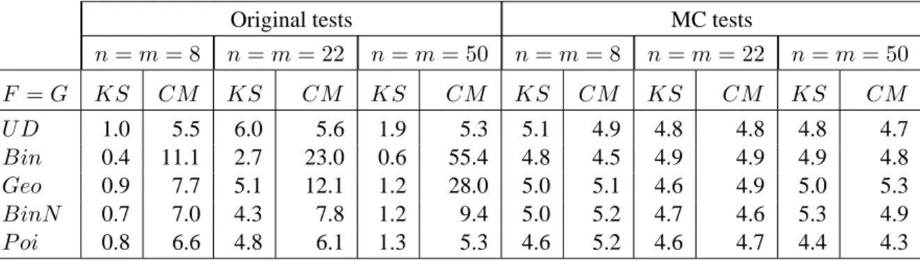
Table 4. Some illustrations for empirical level for KS and CM tests of equality of two discrete distributions (α = 0.05)
Original tests MC tests
n = m = 8 n = m = 22 n = m = 50 n = m = 8 n = m = 22 n = m = 50 F = G KS CM KS CM KS CM KS CM KS CM KS CM U D 1.0 5.5 6.0 5.6 1.9 5.3 5.1 4.9 4.8 4.8 4.8 4.7 Bin 0.4 11.1 2.7 23.0 0.6 55.4 4.8 4.5 4.9 4.9 4.9 4.8 Geo 0.9 7.7 5.1 12.1 1.2 28.0 5.0 5.1 4.6 4.9 5.0 5.3 BinN 0.7 7.0 4.3 7.8 1.2 9.4 5.0 5.2 4.7 4.6 5.3 4.9 P oi 0.8 6.6 4.8 6.1 1.3 5.3 4.6 5.2 4.6 4.7 4.4 4.3
results on this issue for the KS and CM tests. For continuous distributions, we see that the standard
KS and CM tests satisfy the level constraint, although the rejection frequencies of the KS test are
in some cases notably lower than the level. This can be explained by the fact the 0.05 level cannot be achieved by a non-randomized procedure (due to the discrete character of the distribution), so that the critical values used correspond to smaller sizes. In the case of discrete distributions, it is of interest to note that the KS test can be quite conservative (as predicted by earlier theoretical results), while the CM test can substantially overreject: the CM test is not generally conservative for discrete distributions. In all cases, irrespective of whether the distributions are continuous or discrete, the permutational MC tests have rejection frequencies essentially identical to their nominal levels (as expected).
Tables 5 to 8 contain the results of our study for the case where both F and G are continuous. The following conclusions can be drawn. First, it is clear the test based on ˆθ1 has little power for detecting distributions that differ through other characteristics than their mean. Two distributions cannot be equal if they do not have the same mean but the converse is not true. Consequently, if the test based on ˆθ1accepts the hypothesis H0, it should not be interpreted as an acceptance of the fact that F = G but rather that these distributions have equal means.
Second, ˆθ2 has the best power for testing the Gaussian distribution against most of the other distributions considered, but it does not perform as well in the other cases.
Thirdly, the ˆL1 and ˆL2 tests behave almost identically and differ slightly from the ˆL∞test. In
the same way, the power of the KS test is not very different from that of the CM test.
Fourth, if we compare the powers of the tests based on edf‘s (KS and CM ) with those based on pdf estimates ( ˆL1, ˆL2 and ˆL∞), we notice some large power differences, one cannot conclude
that a test from one group is more powerful than all the tests in the other group. The edf tests are more powerful than those based on pdf estimates when two distributions have the same variance but different means (see Tables 2 and 6). On the other hand, if the two distributions have the same mean but different variances, the tests based on pdf estimates are the most powerful (see Tables 2 and 7). Fifth, the combined MC tests exhibit a robust performance in the sense that their power is either the best or is only slightly lower than the one of any other test. There is no uniform dominance
between the test based on the smaller set of statistics ( bQ1) and the one based on the larger one ( bQ2). Not surprisingly, bQ2tends to perform better than bQ1when the distributions compared have different variances (because ˆθ2is used by bQ2but not by bQ1). The combined statistics bQ and bQaexhibit very
similar behaviors, so there appears to be little ground for preferring one over the other.
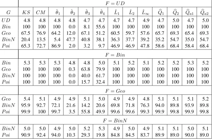
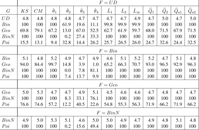
Let us now consider the case where both F and G are discrete. The results of our simulation are presented in Tables 9 to 11. From a qualitative viewpoint, the conclusions that emerge from these are quite similar to those reached in the continuous case: size is perfectly controlled by the MC test technique, the powers of different tests can differ widely depending on the case considered, no test procedure uniformly dominates the others, and the combined test procedures exhibit a good robust overall performance.
6.
Conclusion
In this paper, we first showed that finite-sample distribution-free two-sample homogeneity tests, for both continuous and discrete distributions, can be easily obtained on combining two techniques: (1) by considering permutational versions of most proposed tests for that problem; (2) by implementing the permutation procedures as Monte Carlo tests with an appropriate tie-breaking technique to take account of the discreteness of the test null distributions. Second, due to the flexibility of the Monte Carlo test technique, we could easily introduce and implement several alternative procedures, in-cluding permutation tests comparing higher-order moments and procedures based on combining several test statistics. Thirdly, in a simulation study, it was shown that the procedures proposed work as expected form the viewpoint of size control, while the new test statistics suggested yield power gains.
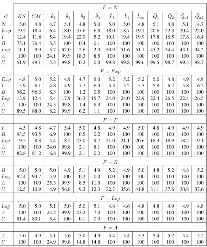
Table 5. Empirical level and power for MC permutation tests of equality of two continuous distributions having same mean and same variance (m = n = 22 and α = 0.05)
F = N G KS CM ˆθ1 ˆθ2 ˆθ3 ˆθ4 Lˆ1 Lˆ2 Lˆ∞ Qb1 Qb2 Qba1 Qba2 N 5.0 4.8 4.7 5.1 4.8 5.0 5.0 5.0 4.8 5.1 4.8 5.1 4.7 Exp 13.8 12.4 5.6 10.5 42.0 15.8 17.3 17.1 15.6 17.1 24.2 17.1 24.1 Γ 8.9 8.8 5.3 7.7 27.0 9.5 11.1 11.0 10.4 10.5 14.2 10.4 14.2 B 5.4 4.9 4.9 5.4 7.5 7.0 5.7 5.9 5.8 5.7 6.4 5.5 6.4 Log 5.7 5.3 5.6 5.1 5.4 6.3 5.3 5.2 5.5 5.4 5.7 5.3 5.7 Λ 71.8 65.2 5.7 59.0 70.2 62.7 68.6 67.6 65.7 79.4 88.9 79.7 88.3 U 6.7 5.7 4.9 6.0 6.4 16.6 6.1 6.5 6.9 6.6 11.1 6.6 11.1 F = Exp Exp 4.8 5.0 5.2 4.9 4.7 5.0 5.2 5.2 5.2 5.0 4.8 4.9 4.9 Γ 6.0 6.0 4.7 5.6 8.3 6.5 6.0 5.9 5.9 6.1 6.8 6.2 6.9 B 11.1 9.1 4.8 12.9 35.9 20.8 15.9 16.0 15.8 15.2 24.6 15.1 24.6 Log 13.4 12.7 5.4 8.5 36.4 11.7 14.5 14.3 12.9 15.3 19.6 15.2 19.5 Λ 85.4 73.1 5.4 50.3 30.6 31.5 54.9 54.6 54.5 86.7 86.8 86.9 86.7 U 17.1 13.7 5.5 17.2 54.8 35.3 22.5 22.7 24.1 23.4 41.5 23.3 41.5 F = Γ Γ 4.5 4.8 4.7 5.4 5.0 4.8 4.9 4.9 5.0 4.8 4.9 4.9 4.9 B 7.3 6.6 5.0 8.8 20.3 12.5 9.8 9.9 9.6 9.2 13.8 9.3 13.8 Log 9.7 8.8 5.5 6.3 23.4 7.4 10.0 10.1 9.3 10.1 11.7 10.0 11.6 Λ 80.5 67.6 5.3 54.2 41.8 42.5 60.9 60.5 60.6 84.1 86.9 84.3 86.7 U 10.5 9.5 5.1 12.6 35.9 25.1 14.6 14.8 15.2 14.0 26.2 13.8 26.2 F = B B 5.0 5.0 5.0 4.9 5.1 4.9 5.2 4.9 5.0 4.8 5.2 4.8 5.2 Log 6.1 5.6 4.7 6.0 8.3 10.9 6.8 6.7 6.9 6.6 9.1 6.6 9.0 Λ 77.2 70.4 5.5 62.5 74.9 70.3 71.8 71.2 69.6 84.0 93.2 84.2 92.8 U 5.5 5.2 5.1 5.4 8.1 10.5 5.6 5.5 5.8 5.6 8.5 5.6 8.5 F = Log Log 5.0 5.0 5.1 5.0 5.0 5.1 4.6 4.6 4.8 4.8 4.9 4.9 4.8 Λ 66.9 59.8 5.8 54.9 60.2 52.6 64.2 63.3 61.2 75.1 83.9 75.4 83.4 U 8.0 6.7 5.2 8.3 8.9 25.6 8.7 9.0 9.6 9.4 16.6 9.3 16.6 F = Λ Λ 5.0 4.9 5.1 5.6 5.0 4.9 5.4 5.4 5.3 5.4 5.2 5.4 5.2 U 82.2 77.4 5.8 65.5 90.3 83.5 76.6 75.6 73.4 88.0 96.5 88.6 96.1
Table 6. Empirical level and power for MC permutation tests of equality of two continuous distributions having different means but same variance (m = n = 22 and α = 0.05)
F = N G KS CM ˆθ1 ˆθ2 ˆθ3 ˆθ4 Lˆ1 Lˆ2 Lˆ∞ Qb1 Qb2 Qba1 Qba2 N 5.0 4.8 4.7 5.1 4.8 5.0 5.0 5.0 4.8 5.1 4.8 5.1 4.7 Exp 90.1 88.9 92.5 5.0 19.3 13.8 38.0 38.6 47.7 83.8 86.6 83.9 86.4 Γ 98.6 99.4 99.9 1.4 14.5 10.2 77.2 77.6 82.2 97.0 98.7 97.1 98.8 B 100 100 100 0.1 7.2 12.4 99.1 99.1 99.4 100 100 100 100 Log 36.1 40.4 42.6 3.8 7.2 8.0 23.6 22.8 21.0 30.4 29.5 30.2 29.4 Λ 88.4 75.7 22.8 55.8 66.0 62.9 68.5 67.8 67.8 90.1 94.0 90.3 93.5 U 99.6 99.9 100 0.1 6.6 18.2 95.2 95.3 96.2 98.9 99.8 98.9 99.8 F = Exp Exp 4.8 5.0 5.2 4.9 4.7 5.0 5.2 5.2 5.2 5.0 4.8 4.9 4.9 Γ 36.9 42.1 30.0 4.5 11.4 9.6 17.9 17.3 15.7 30.8 27.1 30.8 27.0 B 90.3 94.0 86.5 4.4 51.4 41.3 78.8 78.5 75.9 87.9 85.5 87.9 85.5 Log 100 100 100 1.9 35.1 18.1 84.3 85.6 92.9 99.9 100 100 100 Λ 93.4 96.0 76.7 18.7 33.7 30.6 60.7 59.4 55.3 90.5 88.9 90.6 88.7 U 67.6 72.7 63.4 12.0 64.2 49.3 61.4 60.8 57.5 66.6 69.1 66.6 69.1 F = Γ Γ 4.5 4.8 4.7 5.4 5.0 4.8 4.9 4.9 5.0 4.8 4.9 4.9 4.9 B 48.5 53.7 48.0 5.5 28.6 20.7 40.5 40.2 36.6 45.1 42.6 45.1 42.6 Log 100 100 100 0.5 32.0 19.8 98.5 98.8 99.6 100 100 100 100 Λ 100 100 93.0 9.6 51.7 47.8 82.6 81.7 80.5 99.9 99.8 99.9 99.8 U 24.7 24.5 19.4 11.7 41.5 30.5 28.0 27.5 24.7 26.9 34.9 26.7 34.9 F = B B 5.0 5.0 5.0 4.9 5.1 4.9 5.2 4.9 5.0 4.8 5.2 4.8 5.2 Log 100 100 100 0.1 17.0 33.8 100 100 100 100 100 100 100 Λ 100 100 98.2 14.2 86.9 79.2 95.7 95.7 96.7 100 100 100 100 U 8.7 10.0 12.6 4.6 6.8 8.2 6.9 7.0 6.8 8.1 9.5 8.0 9.5 F = Log Log 5.0 5.0 5.1 5.0 5.0 5.1 4.6 4.6 4.8 4.8 4.9 4.9 4.8 Λ 100 99.5 93.3 41.8 66.4 57.6 76.0 75.7 79.9 99.9 99.9 99.9 99.9 U 100 100 100 0.0 14.9 43.4 99.8 99.8 99.9 100 100 100 100 F = Λ Λ 5.0 4.9 5.1 5.6 5.0 4.9 5.4 5.4 5.3 5.4 5.2 5.4 5.2 U 100 100 96.4 45.9 91.5 81.0 91.4 91.3 92.9 100 100 100 100
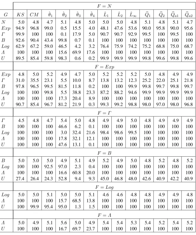
Table 7. Empirical level and power for MC permutation tests of equality of two continuous distributions having same mean but different variances (m = n = 22 and α = 0.05)
F = N G KS CM ˆθ1 ˆθ2 ˆθ3 ˆθ4 Lˆ1 Lˆ2 Lˆ∞ Qb1 Qb2 Qba1 Qba2 N 5.0 4.8 4.7 5.1 4.8 5.0 5.0 5.0 4.8 5.1 4.8 5.1 4.7 Exp 19.2 18.4 6.4 18.0 37.6 6.8 18.0 18.7 19.1 20.6 22.3 20.4 22.0 Γ 12.4 11.8 5.4 19.4 22.9 5.2 19.1 19.4 19.9 17.8 16.5 17.6 16.4 B 75.1 76.4 5.5 100 0.4 0.1 100 100 100 100 100 100 100 Log 11.1 9.9 5.7 57.0 2.6 2.3 50.9 51.6 51.1 43.2 34.4 43.1 34.2 Λ 100 100 24.1 99.9 18.3 8.5 100 100 100 100 100 100 100 U 51.9 49.1 5.3 99.8 0.2 0.0 99.8 99.8 99.6 99.5 98.7 99.5 98.7 F = Exp Exp 4.8 5.0 5.2 4.9 4.7 5.0 5.2 5.2 5.2 5.0 4.8 4.9 4.9 Γ 5.9 6.1 4.8 4.9 7.7 6.0 5.3 5.2 5.3 5.8 6.2 5.8 6.2 B 96.2 96.3 8.3 100 1.2 0.5 100 100 100 100 100 100 100 Log 13.9 12.4 5.4 17.9 36.3 15.7 24.0 24.0 22.9 22.4 26.5 22.4 26.5 Λ 100 100 24.5 99.8 1.4 8.3 100 100 100 100 100 100 100 U 89.5 88.0 8.2 99.9 6.2 1.1 100 100 100 100 100 100 100 F = Γ Γ 4.5 4.8 4.7 5.4 5.0 4.8 4.9 4.9 5.0 4.8 4.9 4.9 4.9 B 93.5 93.5 6.9 100 0.5 0.2 100 100 100 100 100 100 100 Log 9.5 8.8 5.4 18.2 23.0 9.7 21.0 21.1 20.6 18.3 18.9 18.2 19.1 Λ 100 100 24.0 99.8 2.1 8.1 100 100 100 100 100 100 100 U 82.8 81.2 6.8 99.9 2.1 0.2 100 100 100 100 100 100 100 F = B B 5.0 5.0 5.0 4.9 5.1 4.9 5.2 4.9 5.0 4.8 5.2 4.8 5.2 Log 92.4 93.7 5.9 100 0.2 0.0 100 100 100 100 100 100 100 Λ 100 100 25.3 99.9 8.5 11.0 100 100 100 100 100 100 100 U 12.5 10.9 4.9 56.8 9.3 12.3 32.7 35.6 41.8 31.1 37.6 30.8 37.6 F = Log Log 5.0 5.0 5.1 5.0 5.0 5.1 4.6 4.6 4.8 4.8 4.9 4.9 4.8 Λ 100 100 24.2 99.9 23.2 7.0 100 100 100 100 100 100 100 U 81.4 80.1 5.4 100 0.1 0.0 100 100 100 100 100 100 100 F = Λ Λ 5.0 4.9 5.1 5.6 5.0 4.9 5.4 5.4 5.3 5.4 5.2 5.4 5.2 U 100 100 24.9 99.8 14.8 14.8 100 100 100 100 100 100 100
Table 8. Empirical level and power for MC permutation tests of equality of two continuous distributions having different means and different variances (m = n = 22 and α = 0.05)
F = N G KS CM ˆθ1 ˆθ2 ˆθ3 ˆθ4 Lˆ1 Lˆ2 Lˆ∞ Qb1 Qb2 Qba1 Qba2 N 5.0 4.8 4.7 5.1 4.8 5.0 5.0 5.0 4.8 5.1 4.8 5.1 4.7 Exp 94.9 96.8 99.0 0.5 15.5 4.0 48.1 47.6 53.6 90.0 95.8 90.0 95.6 Γ 99.9 100 100 0.1 17.9 5.0 90.7 90.7 92.9 99.5 100 99.5 100 B 92.6 90.4 43.4 99.8 0.7 0.1 100 100 100 100 100 100 100 Log 62.9 67.2 59.0 46.5 4.2 3.2 76.4 75.9 74.2 75.2 68.8 75.0 68.7 Λ 100 100 100 15.6 69.9 17.6 100 100 100 100 100 100 100 U 89.5 85.4 59.8 98.3 0.6 0.2 99.9 99.9 99.9 99.8 99.6 99.8 99.6 F = Exp Exp 4.8 5.0 5.2 4.9 4.7 5.0 5.2 5.2 5.2 5.0 4.8 4.9 4.9 Γ 31.0 35.5 23.1 5.5 10.0 8.7 13.8 13.2 12.3 25.2 22.0 25.1 21.8 B 97.8 96.5 99.5 81.5 11.8 0.2 100 100 99.9 99.8 99.7 99.8 99.7 Log 100 100 99.8 5.5 38.8 23.3 87.2 88.2 94.6 99.9 99.9 99.9 99.9 Λ 100 100 100 17.3 20.4 8.9 100 100 100 100 100 100 100 U 90.7 85.4 96.7 81.2 21.9 0.3 99.3 99.2 98.8 98.0 97.0 98.0 96.8 F = Γ Γ 4.5 4.8 4.7 5.4 5.0 4.8 4.9 4.9 5.0 4.8 4.9 4.9 4.9 B 100 100 100 46.6 6.2 0.1 100 100 100 100 100 100 100 Log 100 100 100 3.0 32.4 21.6 98.4 98.6 99.5 100 100 100 100 Λ 100 100 100 17.8 32.1 12.1 100 100 100 100 100 100 100 U 100 100 100 47.6 13.1 0.1 100 100 100 100 100 100 100 F = B B 5.0 5.0 5.0 4.9 5.1 4.9 5.2 4.9 5.0 4.8 5.2 4.8 5.2 Log 100 100 92.5 97.0 2.3 0.4 100 100 100 100 100 100 100 Λ 100 100 100 16.6 60.8 20.0 100 100 100 100 100 100 100 U 27.4 26.4 24.3 52.8 9.4 9.3 45.0 46.8 48.0 42.6 40.9 42.2 40.9 F = Log Log 5.0 5.0 5.1 5.0 5.0 5.1 4.6 4.6 4.8 4.8 4.9 4.9 4.8 Λ 100 100 100 15.7 68.5 13.8 100 100 100 100 100 100 100 U 100 99.9 95.4 95.0 1.3 1.5 100 100 100 100 100 100 100 F = Λ Λ 5.0 4.9 5.1 5.6 5.0 4.9 5.4 5.4 5.3 5.4 5.2 5.4 5.2 U 100 100 100 16.7 69.7 23.7 100 100 100 100 100 100 100
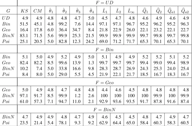
Table 9. Empirical level and power for MC permutation tests of equality of two discrete distributions having same mean but different variances (m = n = 22 and α = 0.05)
F = U D G KS CM ˆθ1 ˆθ2 ˆθ3 ˆθ4 Lˆ1 Lˆ2 Lˆ∞ Qb1 Qb2 Qba1 Qba2 U D 4.9 4.9 4.8 4.8 4.7 5.0 4.5 4.7 4.8 4.6 4.9 4.6 4.9 Bin 51.5 45.1 4.8 99.2 7.6 14.4 97.1 97.1 96.7 95.2 96.2 95.2 96.3 Geo 16.4 17.8 6.0 36.4 34.7 8.4 21.8 22.9 26.0 22.1 23.2 22.1 22.7 BinN 83.1 71.5 5.6 99.9 25.3 21.5 99.9 99.9 99.9 99.7 99.8 99.7 99.8 P oi 25.1 20.5 5.0 82.8 12.3 24.2 69.0 71.2 71.7 65.3 70.1 65.3 70.1 F = Bin Bin 5.1 5.0 4.9 5.2 4.9 5.0 5.1 4.9 4.9 5.2 5.2 5.1 5.2 Geo 82.4 82.2 8.5 99.6 13.9 1.3 99.7 99.7 99.7 99.4 99.0 99.4 98.9 BinN 10.2 7.4 5.0 33.8 16.6 9.8 28.3 28.7 26.9 24.3 25.3 24.0 25.4 P oi 8.4 8.0 5.0 29.0 5.5 4.5 21.9 22.1 21.7 18.5 16.7 18.3 16.7 F = Geo Geo 5.0 4.9 4.8 4.7 4.8 4.8 4.4 4.6 4.5 4.8 4.8 4.8 4.8 BinN 97.1 91.7 8.5 99.9 1.2 2.6 100 100 100 100 99.9 100 99.9 P oi 61.0 57.3 7.1 94.7 11.0 2.1 92.9 93.6 93.5 91.7 87.8 91.6 87.4 F = BinN BinN 4.7 4.9 4.9 4.8 4.7 4.9 4.6 4.5 4.5 4.8 4.7 4.9 4.7 P oi 23.5 21.4 5.4 78.1 9.3 9.2 62.9 64.4 65.0 58.4 60.3 58.3 60.5
Table 10. Empirical level and power for MC permutation tests of equality of two discrete distributions having different means and same variance (m = n = 22 and α = 0.05)
F = U D G KS CM ˆθ1 ˆθ2 ˆθ3 ˆθ4 Lˆ1 Lˆ2 Lˆ∞ Qb1 Qb2 Qba1 Qba2 U D 4.8 4.8 4.8 4.8 4.7 4.7 4.7 4.7 4.9 4.7 5.0 4.7 5.0 Bin 100 100 100 0.0 8.1 55.6 100 100 100 100 100 100 100 Geo 67.5 76.9 64.2 12.0 67.1 51.2 60.5 59.7 57.6 65.7 69.3 65.4 69.3 BinN 20.4 13.5 5.4 47.7 40.8 38.1 36.3 37.7 39.2 35.2 54.7 35.0 54.7 P oi 65.3 72.7 86.9 2.0 3.2 9.7 46.9 46.9 47.8 58.6 68.4 58.4 68.4 F = Bin Bin 5.3 5.3 5.3 4.8 4.8 5.0 5.1 5.2 5.1 5.2 5.2 5.3 5.2 Geo 100 100 100 0.3 63.8 79.9 100 100 100 100 100 100 100 BinN 100 100 100 0.0 40.0 61.7 100 100 100 100 100 100 100 P oi 100 100 100 0.0 15.7 32.4 100 100 100 100 100 100 100 F = Geo Geo 5.4 5.1 4.9 4.9 5.1 5.0 4.9 4.9 4.8 5.1 5.1 5.1 5.2 BinN 95.9 92.7 72.1 21.6 14.2 20.6 69.8 71.8 76.3 94.0 89.8 93.9 89.8 P oi 99.9 100 99.7 3.5 55.8 49.9 99.6 99.6 99.3 99.9 99.8 99.9 99.8 F = BinN BinN 5.0 5.0 4.9 5.0 5.2 5.3 4.9 5.0 4.9 5.1 5.1 5.0 5.1 P oi 90.9 92.4 94.0 10.3 29.3 19.8 84.8 84.5 83.7 89.9 89.0 90.0 89.0
Table 11. Empirical level and power for MC permutation tests of equality of two discrete distributions having different means and different variances (m = n = 22 and α = 0.05)
F = U D G KS CM ˆθ1 ˆθ2 ˆθ3 ˆθ4 Lˆ1 Lˆ2 Lˆ∞ Qb1 Qb2 Qba1 Qba2 U D 4.8 4.8 4.8 4.8 4.7 4.7 4.7 4.7 4.9 4.7 5.0 4.7 5.0 Bin 100 100 100 61.9 19.6 11.1 99.8 99.9 99.9 100 100 100 100 Geo 69.8 79.1 67.2 13.0 67.0 52.5 62.7 61.9 59.7 68.0 71.5 67.9 71.5 BinN 100 100 100 0.2 27.4 33.3 100 100 100 100 100 100 100 P oi 15.5 13.1 9.4 32.8 14.4 26.2 25.7 26.5 26.0 24.7 32.6 24.4 32.5 F = Bin Bin 5.1 4.8 5.2 4.9 4.7 4.9 4.6 5.1 5.2 5.2 4.7 5.1 4.8 Geo 94.0 84.4 99.7 14.8 3.9 1.0 65.2 66.3 70.7 93.0 96.5 92.9 96.3 BinN 100 100 100 0.0 7.8 81.1 100 100 100 100 100 100 100 P oi 100 100 100 7.4 13.7 9.9 100 100 100 100 100 100 100 F = Geo Geo 5.0 5.3 4.7 4.7 4.9 5.1 4.5 4.6 4.6 4.7 4.8 4.7 4.7 BinN 100 100 100 8.3 33.1 76.1 100 100 100 100 100 100 100 P oi 76.6 74.6 57.2 12.2 40.5 22.6 54.8 55.3 56.3 71.9 66.2 71.9 66.2 F = BinN BinN 4.9 5.0 5.3 5.1 4.6 5.0 5.0 4.9 4.7 4.9 4.8 5.1 4.8 P oi 100 100 100 0.2 15.6 49.4 100 100 100 100 100 100 100
References
Allen, D. L. (1997), ‘Hypothesis testing using an L1-distance bootstrap’, The American Statistician
51, 145–150.
Anderson, T. W. (1962), ‘On the distribution of the two-sample Cramér-von Mises criterion’, Annals
of Mathematical Statistics 33, 1148–1159.
Anderson, T. W. and Darling, D. A. (1952), ‘Asymptotic theory of certain ‘goodness of fit’ criteria based on processes’, Annals of Mathematical Statistics 23, 193–212.
Barnard, G. A. (1963), ‘Comment on ‘The spectral analysis of point processes’ by M. S. Bartlett’,
Journal of the Royal Statistical Society, Series B 25, 294.
Barton, D. E. and Mallows, C. L. (1965), ‘Some aspects of the random sequence’, Annals of
Math-ematical Statistics 36, 236–260.
Birnbaum, Z. W. (1974), Computers and unconventional test-statistics, in F. Proschan and R. J. Serfling, eds, ‘Reliability and Biometry’, SIAM, Philadelphia, PA, pp. 441–458.
Birnbaum, Z. W. and Hall, R. A. (1960), ‘Small sample distributions for multi-sample statistics of the Smirnov type’, Annals of Mathematical Statistics 31, 710–720.
Burr, E. J. (1963), ‘Distribution of the two-sample Cramér-von Mises criterion for small equal samples’, Annals of Mathematical Statistics 34, 95–101.
Burr, E. J. (1964), ‘Small samples distributions of the two-sample Cramér-von Mises’ W2 and Watson’s U2’, Annals of Mathematical Statistics 35, 1091–1098.
Conover, W. J. (1971), Practical Nonparametric Statistics, John Wiley & Sons, New York.
Darling, D. A. (1957), ‘The Kolmogorov-Smirnov, Cramér-von Mises tests’, Annals of
Mathemati-cal Statistics 28, 223–238.
Davison, A. and Hinkley, D. (1997), Bootstrap Methods and Their Application, Cambridge Univer-sity Press, Cambridge (UK).
Drion, E. F. (1952), ‘Some distribution free tests for the difference between two empirical cumula-tive distributions’, Annals of Mathematical Statistics 23, 563–564.
Dufour, J.-M. (1989), ‘Nonlinear hypotheses, inequality restrictions, and non-nested hypotheses: Exact simultaneous tests in linear regressions’, Econometrica 57, 335–355.
Dufour, J.-M. (1990), ‘Exact tests and confidence sets in linear regressions with autocorrelated errors’, Econometrica 58, 475–494.
Dufour, J.-M. (1995), Monte Carlo tests with nuisance parameters: A general approach to finite-sample inference and nonstandard asymptotics in econometrics, Technical report, C.R.D.E., Université de Montréal.
Dufour, J.-M., Farhat, A., Gardiol, L. and Khalaf, L. (1998), ‘Simulation-based finite sample nor-mality tests in linear regressions’, The Econometrics Journal 1, 154–173.
Dufour, J.-M. and Khalaf, L. (2001), Monte Carlo test methods in econometrics, in B. Baltagi, ed., ‘Companion to Theoretical Econometrics’, Blackwell Companions to Contemporary Eco-nomics, Basil Blackwell, Oxford, U.K., chapter 23, pp. 494–519.
Dufour, J.-M. and Kiviet, J. F. (1998), ‘Exact inference methods for first-order autoregressive dis-tributed lag models’, Econometrica 66, 79–104.
Dufour, J.-M. and Torrès, O. (1998), Union-intersection and sample-split methods in econometrics with applications to SURE and MA models, in D. E. A. Giles and A. Ullah, eds, ‘Handbook of Applied Economic Statistics’, Marcel Dekker, New York, pp. 465–505.
Dufour, J.-M. and Torrès, O. (2000), ‘Markovian processes, two-sided autoregressions and exact inference for stationary and nonstationary autoregressive processes’, Journal of Econometrics
99, 255–289.
Dwass, M. (1957), ‘Modified randomization tests for nonparametric hypotheses’, Annals of
Mathe-matical Statistics 28, 181–187.
Efron, B. and Tibshirani, R. J. (1993), An Introduction to the Bootstrap, Vol. 57 of Monographs on
Statistics and Applied Probability, Chapman & Hall, New York.
Fisher, R. A. (1935), The Design of Experiments, Oliver and Boyd, London.
Fisz, M. (1960), ‘On a result by M. Rosenblatt concerning the Mises-Smirnov test’, Annals of
Mathematical Statistics 31, 427–429.
Folks, J. L. (1984), Combination of independent tests, in P. R. Krishnaiah and P. K. Sen, eds, ‘Handbook of Statistics 4: Nonparametric Methods’, North-Holland, Amsterdam, pp. 113– 121.
Foutz, R. V. (1980), ‘A method for constructing exact tests from test statistics that have unknown null distributions’, Journal of Statistical Computation and Simulation 10, 187–193.
Gibbons, J. D. and Chakraborti, S. (1992), Nonparametric Statistical Inference, Third Edition,
Re-vised and Expanded, Marcel Dekker, New York.
Gnedenko, B. V. (1954), ‘Tests of homogeneity of probability distributions in two independent samples (in Russian)’, Doklady Akademii Nauk SSSR 80, 525–528.
Goodman, L. A. (1954), ‘Kolmogorov-Smirnov tests for psychological research’, Psychological
Bulletin 51, 160–168.
Hájek, J. and Šidák, Z. (1967), Theory of Rank Tests, Academic Press, New York. Hall, P. (1992), The Bootstrap and Edgeworth Expansion, Springer-Verlag, New York.
Hodges, Jr., J. L. (1958), ‘The significance probability of Smirnov two-sample test’, Arkivfoer
Matematik, Astronomi och Fysik 3, 469–486.
Jarque, C. M. and Bera, A. K. (1987), ‘A test for normality of observations and regression residuals’,
International Statistical Review 55, 163–172.
Jöckel, K.-H. (1986), ‘Finite sample properties and asymptotic efficiency of Monte Carlo tests’, The
Annals of Statistics 14, 336–347.
Kim, P. J. (1969), ‘On the exact and approximate sampling distributions of the two sample Kolmogorov-Smirnov crirerion Dmn, m ≤ n’, Journal of the American Statistical
Associ-ation 64, 1625–1637.
Kim, P. J. and Jennrich, R. I. (1970), Tables of the exact distribution of the two sample Kolmogorov-Smirnov crirerion Dmn, m ≤ n, in H. L. Harter and D. B. Owen, eds, ‘Selected Tables in
Methematical Statistics’, Vol. 1, American Mathematical Society, Providence, Rhode Island, pp. 79–170.
Kiviet, J. and Dufour, J.-M. (1997), ‘Exact tests in single equation autoregressive distributed lag models’, Journal of Econometrics 80, 325–353.
Korolyuk, V. S. (1961), ‘On the discrepancy of empiric distributions for the case of two independent samples’, Selected Translations in Mathematical Statistics and Probability 1, 105–121. Lehmann, E. L. (1951), ‘Consistency and unbiasedness of certain nonparametric tests’, Annals of
Mathematical Statistics 22, 165–179.
Lehmann, E. L. (1986), Testing Statistical Hypotheses, 2nd edition, John Wiley & Sons, New York. Massey, F. J. (1951a), ‘The distribution between of the maximum deviation between two sample
cumulative step functions’, Annals of Mathematical Statistics 22, 125–128.
Massey, F. J. (1951b), ‘A note on a two sample test’, Annals of Mathematical Statistics 22, 304–306. Massey, F. J. (1952), ‘Distribution table for the deviation between two sample cumulatives’, Annals
of Mathematical Statistics 23, 435–441.
Miller, Jr., R. G. (1981), Simultaneous Statistical Inference, second edn, Springer-Verlag, New York. Noether, G. E. (1963), ‘Note on the Kolmogorov statistic in the discrete case’, Metrika 7, 115–116. Pitman, E. J. G. (1937), ‘Significance tests which may be applied to samples from any populations’,
Journal of the Royal Statistical Society, Series A 4, 119–130.
Rosenblatt, M. (1952), ‘Limit theorems associated with variants of the von Mises statistic’, Annals
of Mathematical Statistics 23, 617–623.
Smirnov, N. V. (1939), ‘Sur les écarts de la courbe de distribution empirique (Russian/French sum-mary)’, Matematiˇceskiˇı Sbornik N.S. 6, 3–26.
Smirnov, N. V. (1948), ‘Table for estimating the goodness of fit of empirical distributions’, Annals
of Mathematical Statistics 19, 279–281.
Steck, G. P. (1969), ‘The Smirnov two sample tests as rank tests’, Annals of Mathematical Statistics
40, 1449–1466.
Walsh, J. E. (1963), ‘Bounded probability properties for Kolmogorov-Smirnov and similar statistics for discrete data’, Annals of the Institute of Statistical Mathematics 15, 153–158.
Westfall, P. H. and Young, S. S. (1993), Resampling-Based Multiple Testing: Examples and Methods