Bellemare: Département d’économique, Université Laval, CIRPÉE
Sebald: Department of Economics, University of Copenhagen
Strobel: Department of Economics, Maastricht University
We thank the team at CentERdata for support throughout the experiment. The first author thanks the Canada Chair of Research in the Economics of Social Policies and Human Resources for support. We also thank Martin Dufwenberg, Chuck Manski, Christoph Vanberg, Sigrid Suetens, and participants at the Workshop on Subjective Expectations in Econometric Models in Québec, as well as participants at conferences in Copenhagen, Haifa, Granada, Maastricht and Oslo for helpful comments and suggestions.
Cahier de recherche/Working Paper 10-11
Measuring the Willingness to Pay to Avoid Guilt: Estimation using
Equilibrium and Stated Belief Models
(Forthcoming, Journal of Applied Econometrics)
Charles Bellemare Alexander Sebald Martin Strobel
Abstract:
We estimate structural models of guilt aversion to measure the population level of willingness to pay (WTP) to avoid feeling guilt by letting down another player. We compare estimates of WTP under the assumption that higher-order beliefs are in equilibrium (i.e. consistent with the choice distribution) with models estimated using stated beliefs which relax the equilibrium requirement. We estimate WTP in the later case by allowing stated beliefs to be correlated with guilt aversion, thus controlling for a possible source of a consensus effect. All models are estimated using data from an experiment of proposal and response conducted with a large and representative sample of the Dutch population. Our range of estimates suggests that responders are willing to pay between 0.40 and 0.80 Euro to avoid letting down proposers by 1 Euro. Furthermore, we find that WTP estimated using stated beliefs is substantially overestimated (by a factor of two) when correlation between preferences and beliefs is not controlled for. Finally, we find no evidence that WTP is significantly related to the observable socio-economic characteristics of players.
Keywords: Guilt aversion, Willingness to pay, Equilibrium and stated beliefs models
1
Introduction
Persistent findings in experimental economics suggest that in many strategic environments people’s preferences do not only depend upon the strategies played but also on the beliefs
they hold about other people’s intentions and expectations (see e.g. Falk, Fehr, and Fis-chbacher, 2008; Charness and Dufwenberg, 2006). One specific type of belief-dependent
preferences which has received a lot of attention recently is guilt aversion (Charness and Dufwenberg, 2006; Battigalli and Dufwenberg, 2007; Vanberg, 2008; Ellingsen,
Johannes-son, Tjøtta, and Torsvik, 2009). In that literature an individual is defined as guilt averse if he values living up to his expectations of what other individuals expect of him. Not
doing so causes a feeling of guilt which negatively affects the individual’s utility and thus influences decision making.
The aim of this paper is to estimate structural models of guilt aversion to measure the level of willingness to pay (WTP) in the Dutch population to avoid feeling guilty.1
Existing works test for the presence of guilt aversion by measuring the correlation between players’ decisions and their second-order beliefs: their expectations of what others expect
of them. The estimated correlations typically suggest significant guilt aversion in student populations (e.g. Charness and Dufwenberg, 2006). While such tests provide indications
of the relevance of guilt aversion, they provide little information concerning the quan-titative importance of guilt aversion relative to self-interest. Measuring WTP thus has
the potential to provide new insights on the quantitative importance of guilt aversion for players.
To proceed, we conducted an experiment with a large and representative sample of the Dutch population. The experiment was based on a simple sequential two player game
of proposal and response with two additional inactive players. In the main treatment (henceforth treatment S) responders made their decisions and were then asked to state
1Hence, this paper relates to recent attempts to measure population parameters using controlled
experiments as opposed to parameters characterizing student populations (see eg. Bellemare, Kr¨oger, and van Soest, 2008).
their second-order beliefs: their expectations of the first-order beliefs of proposers.
Measuring WTP using stated second-order beliefs and decisions from treatment S raises some important issues. In particular, it has recently been argued that observing a
significant correlation between responders’ decisions and their stated second-order beliefs does not necessarily imply guilt aversion (see Charness and Dufwenberg, 2006; Vanberg,
2008; Ellingsen, Johannesson, Tjøtta, and Torsvik, 2009). The observed correlation may instead reflect a consensus effect which occurs when individuals condition on their behavior
(and preferences) when stating their beliefs (Ross, Greene and House, 1977).2 This effect has been thoroughly studied in psychology. For our simple game it means that responders’
stated second-order beliefs are affected by their intended decisions rather than vice-versa. We address these issues by jointly modeling decisions and stated second-order beliefs of
players in treatment S, allowing for correlation between guilt aversion and stated beliefs.3 We use our estimated model to quantify how much of the estimated WTP is due to
genuine guilt aversion, and how much is due to correlation between preferences and stated beliefs. Furthermore, we compare our estimates of WTP obtained using stated beliefs
with those obtained using decisions and beliefs in treatment X. Treatment X is identical to treatment S except that responders where informed about the true first-order beliefs of
proposers before they made their decisions. Hence, second-order beliefs and preferences of responders in treatment X are uncorrelated by design.4 The comparison of our estimates
in treatment S with those of treatment X will provide further indication of the possible bias in estimated WTP which results from correlation between preferences and stated
2We will call it a consensus effect although in the original definition Ross, Greene and House (1977)
speak of a false consensus effect. Dawes (1989, 1990) argues that the label false is not justified because the effect can be rationalized in a Bayesian framework. Engelmann and Strobel (2000) experimentally investigate this issue and found clear evidence against the falsity. For our purpose this distinction is however secondary.
3A similar econometric approach was followed by Bellemare, Kr¨oger, and van Soest (2008). There,
they estimate a structural model of choice under uncertainty using ultimatum game data where beliefs are allowed to be correlated with inequity averse preferences.
beliefs.
In the final part of the paper we estimate WTP assuming that beliefs are consistent with the relevant choice distributions. This equilibrium approach is especially appealing
for two reasons. First, it is firmly grounded in theory (see e.g. Harsanyi 1967, Battigalli and Dufwenberg, 2007 and Battigalli and Dufwenberg, 2009).5 Second, the consistency
requirement closes the model and thus circumvents the need to collect data on (higher-order) beliefs. As a result, the equilibrium approach avoids possible biases due to
consen-sus effects which arise when using stated beliefs. Obviously, one potential drawback of the equilibrium approach is that the consistency of decisions and beliefs may be an overly
restrictive assumption in one shot games as players do not have any opportunity to learn about the expectations of others. In fact, we will show that the assumption that beliefs
are in equilibrium appears to be rejected by the data. Hence, our goal is to investigate whether the equilibrium model can nevertheless provide reasonable estimates of WTP as
a first approximation.
Our main results are the following. First, we find that the estimated WTP is
signifi-cantly higher (by a factor of 2) in treatment S than in treatment X when we do not control for correlation between stated beliefs and preferences in treatment S. However, the
esti-mated WTP using stated beliefs is substantially smaller (but remains significant) once controlling for this correlation. In fact, controlling for correlation between preferences
and beliefs produces estimates of WTP in treatment S which are closer in magnitude and insignificantly different from the level of WTP estimated in treatment X. These result
suggest that ignoring correlation between preferences and beliefs can result in important overestimation of WTP when using stated beliefs. Second, our range of estimates suggests
that responders are on average willing to pay between 0.40 Euro and 0.80 Euro to avoid letting down proposers by 1 Euro. Third, the WTP estimated under the assumption that
5Theoretical models of guilt aversion do not necessary require that beliefs be in equilibrium to generate
predictions about behavior. Battigalli and Dufwenberg (2009) for example also analyze strategic behavior in psychological games under the weaker requirement that beliefs are rationalizable. See their section 5.2 for a discussion.
beliefs are in equilibrium is significant and falls within this range of estimates. Fourth, we
do not find that WTP to avoid letting down any player varies significantly across various socio-economic dimensions (age, education, income, etc.).6 Finally, we find no evidence
that second movers are willing to pay to avoid letting down inactive players. This result holds for both the stated and equilibrium belief models.
The organization of the paper is as follows. In section 2 we describe the game and experimental setup. In section 3 we present our data. Section 4 presents a model of
simple guilt. Section 5 presents our econometric model using stated beliefs while section 6 presents our econometric model assuming equilibrium beliefs. Section 7 concludes.
2
The Game and the Experimental Setup
The experiment was conducted via the CentERpanel, an Internet survey panel managed by CentERdata at Tilburg University. The panel consists of about 4000 households, a
representative sample of the Dutch population. Households are contacted every Friday and are asked to answer several questions. Members of each household have until Sunday
night to respond. Most of these questions are survey questions about household decisions but CentERdata also allows for simple interactive experiments.7 Our experiment is based
on the following game:
6Recent experimental studies sampling the same population (Bellemare and Kr¨oger, 2007;,
Belle-mare, Kr¨oger, and van Soest, 2008) have on the other hand found that distributional preferences vary significantly across socio-economic dimensions.
7For more details and a description of the recruitment, sampling methods, and past usages of the
CentERpanel see: www.centerdata.nl. Computer screens from the original experiment (in Dutch) with translations are available upon request.
Player A L @@ R @ @ Player B l @@ r @ @ yA(l) yB(l) yC(l) yD(l) yA(r) yB(r) yC(r) yD(r) xA(R) xB(R) xC(R) xD(R)
In this simple sequential game, there are four players: A, B, C and D. Player A can choose either the outside option R or he can choose L to let player B decide. If player A
chooses R then the game ends and the players receive their payoffs xA(R), xB(R), xC(R) and xD(R), respectively. If player A decides to choose L then player B has to choose
either l or r. In both cases the game ends and the players receive their corresponding payoffs, either yA(l), yB(l), yC(l) and yD(l), respectively or yA(r), yB(r), yC(r) and yD(r),
respectively.
Players C and D are dummy players whose monetary payoffs are determined by the
choices of player A and (possibly) B.8 We included C and D players to analyze how B’s decision is affected by the presence of strategically uninvolved players. The existing
literature (e.g. G¨uth and Van Damme, 1998; Kagel and Wolfe, 2001) indicates that the presence of one inactive player has a weak influence of behavior in simple games. Here,
we use two inactive players in order to make their presence in the game more salient. Payoffs were systematically varied across games with the help of Optimal Design Theory
(see Mueller and Ponce de Leon, 1996). Payoffs were presented in CentERpoints - the currency that is usually used in experiments conducted with the CentERpanel. In total
8Our game is similar to that analyzed by Charness and Rabin (2005) with the difference that we
include the dummy players C and D. Furthermore, contrary to them, A players in our experiment could not communicate to B players their preferences over the possible choices of B players.
we invited 3000 panel members to participate for both treatments. From all invited
participants, 1962 responded and went through the whole experiment. We next describe both treatments of our experiment in detail.
Treatment S
Treatment S was conducted at the beginning of 2007. We invited 2000 CentERpanel members to participate in this treatment. 1666 out of the 2000 invited panel members
responded to the invitation by reading the opening screens of the experiment. They were provided with a description of the game, the possible choices that players in the
different roles could make and their associated consequences. Before the revelation of their roles and monetary payoffs, members were given the chance to resign from the
experiment. 264 members resigned at this stage, leaving us with 1402 members who where then randomly assigned to a specific game and to one of the four different roles
A, B, C and D. Following the information about their role and their game’s payoffs,
participants were asked to make their choices. We used the strategy method (see Selten
1967). This means that A and B players made their decisions separately, which B players
asked to make a decision conditional on player A choosing L. This helped us overcome the problems of coordinating interactions in real time via the panel.
After making their decision, A players was asked to state their first-order beliefs
con-cerning the behavior of player B if they chose to let this player decide the final allocation.9
In particular, A players were presented the following question
(First-order beliefs of A players) What do you think, how many B-Persons out of 100 will choose l and how many r. Please indicate this number for each possible allocation.
1. Number of B Persons out of 100 that will choose B.1 : XA
2. Number of B Persons out of 100 that will choose B.2 : YA
9 Asking beliefs after their decisions implies that the later are unaffected by the belief elicitation. As
a result, we are able to use the decisions of B players in treatment S to estimate the equilibrium model presented in Section 6.
The computer program automatically ensured that the numbers entered (XA+YA) added
up to 100. To simplify the task of participants, all beliefs were elicited using natural frequencies.10
After their decisions (l or r), B players were asked to state their second-order beliefs. In particular, they were asked to answer the following question:
(Second-order beliefs of B players) What do you think about Person A’s beliefs about the behavior of Persons B? Please indicate this number for each possible allocation.
1. Person A believes that XB B-Persons out of 100 choose B.1
2. Person A believes that YB B Persons out of 100 choose B.2
Again, the computer program automatically ensured that the numbers XB+ YB added up to 100.11 We did not pay players for accuracy of their beliefs.12
The decisions of A and B players were matched after the experiment to determine the final payoff of all players. Before the experiment participants were informed that we
expect at most 2000 persons to participate and 50 played games (50 players of each role) would be paid.13 In order to increase the number of B-player decisions which were most
interesting for us, we put more persons into the role of B than into the other roles. More
10This follows Hoffrage, Lindsey, Hertwig, and Gigerenzer (2000) who found that people are better at
working with natural frequencies than with percent probabilities.
11Our elicitation procedure elicits a single point of the subjective distribution of the beliefs of B
players. There is uncertainty over the interpretation of these point estimates. Recent research suggests that respondents may interpret differently the belief question. As a result, they may report different points (eg. means, medians, modes) of their subjective distribution. See Manski (2004) for a recent review.
12Several studies have found that rewarding subjects for the accuracy of their expectations using
an incentive compatible scoring rule does not produce significantly different elicited expectations; see Friedman and Massaro (1998) and Sonnemans and Offerman (2001).
13The experiment was conducted using CentERpoints, the usual currency for CentERpanel members.
For the sake of simplicity we state directly the amounts in Euro. The exchange-rate was 100 CentERpoints = 1e.
specifically, we had prepared 1600 payoff-wise different games for treatment S. Given these
1600 games, we decided a priori to randomly allocate each of our initial 2000 invited panel members to one of the four roles in the following proportions: 1600 B player roles (one for
each game), 300 A players, 50 C players, and 50 D-players. We randomly picked 50 out of the 300 games consisting of A and a B players to which we assigned C and D players.
This means, we a priori randomly picked 50 payoff-wise different games (out of 1600) and paid all players in those selected games. Hence, in the beginning of the experiment
participants were randomly allocated to a specific role and a game ensuring that a-priori everybody had an equal chance to be in a game which was paid off at the end (for
details see also the translated screens of the experiment in the appendix). As announced before the experiment, participants of the games that were paid out received information
on the outcome of their game and their final payoffs a few weeks after the experiment. Furthermore, the corresponding amounts were credited to their bank accounts. Of the
1402 participants that completed the experiment there were 1114 B players, 214 A players and 74 C and D players.14
Treatment X
Treatment X was conducted during the summer of 2008. For this treatment, we (i) selected all 214 games in treatment S with decisions and stated first-order beliefs of A players, (ii)
we re-contacted the A, C and D players who had played these specific games and asked them whether we could use their decisions and beliefs (if any) for a follow-up experiment
and (iii) invited 1000 new members of the CentERpanel to participate in the experiment. Note, in order to avoid any deception, all A, C and D players that were recontacted
were given the possibility to decline, preventing us to use their decisions and beliefs. No player declined our request. Furthermore, 719 out of the 1000 new invited panel members
responded to the invitation by reading the opening screens of the experiment. As in
14Table 1 presents data from treatment S. As can be seen, the sample size of treatment S is N=1078.
1078 represents the number of B players (out of the 1114) for whom we had a complete record of background characteristics.
treatment S, they were given the chance to resign from the experiment after the structure
of the game was explained but before they learned their role and the detailed payoffs. 159 members resigned at this stage, leaving us with 560 new members who where then all
assigned to the role of player B and confronted with their specific game.15 In contrast to treatment S, the B players in treatment X were not asked for their second-order beliefs but
were presented the first-order beliefs of their matched A player (taken from treatment S) before making their decisions. All other features of the treatment are otherwise identical
to treatment S. We informed participants before the experiment that 25 games played were going to be randomly selected and paid. As before the subjects received information
about the decisions a few weeks later and for the players of the selected games including
A, C and D players the corresponding amounts were credited to their bank account.
3
Data
Table 1 presents the sample means and standard deviations of the allocations to A, B, C, and D players at the three end nodes of the game. The average allocation ranges between
20 and 25 Euros per player depending on the role and the terminal node.
First-order beliefs of A players were elicited in treatment S and are provided to
B-players in treatment X. We analyze the first-order beliefs of A B-players in treatment S by estimating the following linear regression
bAi = α0+ α1∆yiA+ α2∆yiB+ α3∆yCi + α4∆yiD+ ϵi (1)
where bA
i denotes the stated probability of player A on player B playing r (first-order
beliefs of player A), and where ∆yik = yik(r)− yik(l) denotes the payoff difference when player B chooses r relative to l for player k ∈ {A, B, C, D}. The estimated equation is
15Hence the 214 games were used on average more than twice. Table 1 presents data from treatment
X. The sample size of treatment X is N=540. Analogous to treatment S, 540 represents the number of
the following (with robust standard errors in parenthesis) bbA i = 0.473 (0.019)+ 0.001(0.001)∆y A i + 0.006∗∗∗ (0.001) ∆y B i + 0.001 (0.001)∆y C i + 0.000 (0.000)∆y D i
We find that A players expect that B players are more likely to choose r the more B players
can benefit from this choice. Interestingly, first-order beliefs do not vary significantly with payoffs of other players. This suggests that A players do not expect that B players will
take into account the well being of other players when making their decisions.
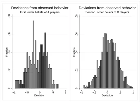
We next investigated whether stated expectations of A and B players are rational, that
is consistent with observable outcomes. We first compared the stated first-order beliefs of A players with the realized choice probabilities of B players. To compute the later, let
pi denote the vector of payoffs differences (ie. ∆yik) of all players involved in the game
played by the i’th player A. Furthermore, let bA
i denote player A’s subjective probability
that player B will chose to play r. We estimated nonparametrically Pr(c = r|pi) for
each player A, where Pr(c = r|pi) denotes the probability that B players choose r given
pi.16 We then computed bAi − cPr(c = r|pi) for each player A, that is the difference
between the stated first-order beliefs of player A and the corresponding estimated choice
probability of B players in the game played by i. The left hand graph of Figure 1 plots the distribution of differences for all A players in treatment S. Rational expectations would
imply a distribution concentrated around zero. We find substantial deviations, suggesting that expectations of A players are far from consistent with the observed choice behavior.
We next compared the stated second-order beliefs of each B player in treatment S (denoted bAi ) with the expected first-order beliefs of A players. To compute the later,
we estimated nonparametrically E(bAi |pi) for each B player, where E(bAi |pi) denotes the
objective expected first-order beliefs of A players given the game played by the i’th player
B. We then computed bAi − bE(bAi |pi) for each i. The right hand graph of Figure 1
presents the deviations for all B players in treatment S. Rational expectations would
again imply that this distribution would be concentrated around zero. However, we also
16All nonparametric regressions use the Nadaraya-Watson estimator with gaussian kernel. See Li and
find substantial deviations, suggesting that stated second-order beliefs of B players are
also inconsistent with the observed first-order beliefs of A players.
4
A model of simple guilt aversion
In this section, we specify a structural econometric model of guilt version. Our starting
point is the model of ‘simple guilt’ proposed by Battigalli and Dufwenberg (2007).17 We
start by assuming that the utility of of choosing r for player B is given by
Ui(r) = yiB(r) + ϕAi GAi (r) + ϕCDi GCDi (r) (2)
where yB
i (r) denotes his payoff, GAi (r) denotes guilt towards player A (conditional on
player A’s beliefs), and where GCDi (r) denotes guilt towards players (C, D) (conditional on players C and D’s beliefs). Player B’s utility of choosing l is defined analogously and
is omitted for brevity. The parameter ϕA
i controls player B’s sensitivity to guilt towards player A. Similarly,
ϕCDi controls player B’s sensitivity to guilt towards players (C, D). Note, as marginal utility of own income yB
i is normalized to 1, the (absolute) values of ϕAi and ϕCDi also
rep-resent player B’s willingness to pay to avoid letting down A and C, D players respectively by 1 CentERpoint.
The guilt variables from choosing r are defined as
GAi (r) = [E(YiA)− yiA(r)]1[yAi (r) < yiA(l)] (3)
GCDi (r) = [E(YiCD)− yiCD(r)]1[yiCD(r) < yiCD(l)] (4) where E(YiA)denotes the expected payoff of player A, where yiCD(n)≡ yiC(n) + yiD(n) for
n ∈ {l, r}, and where E(YCD i
)
denotes the expectation of the sum of payoffs of players
17Note, Battigalli and Dufwenberg (2007) also present an extended model of ‘guilt from blame’ which
assumes that a player cares about others inferences regarding the extent to which he is willing to let down.
C and D.18 These expectations are given by E(YiA) = bAi yAi (r) + (1− bAi )yiA(l) (5) = bAi [yiA(r)− yAi (l)]+ yiA(l) E(YiCD) = bCDi yiCD(r) + (1− bCDi )yiCD(l) (6) = bCDi [yiCD(r)− yiCD(l)]+ yiCD(l) where bA
i denotes player A’s subjective belief that player B will play r, while bCDi denotes
players C and D’s subjective belief that player B will play r. Player B ‘lets down’ player
A by choosing r if this provides player A with a final payoff yA
i (r) below his expectation.
Similarly, player B ‘lets down’ players C and D by choosing r if this provides these players with a final payoff yCD
i (r) below their expectation. Hence, we assume that a player cares
about the extent to which he lets other players down, where GAi (r) and GCDi (r) measure the amount of let down from choosing r. From (2), (3), and (4) it also follows that player
i can only let down player A (or players CD) by choosing the alternative providing A (or
players CD) with his lowest payoff.19
So far, the analysis has assumed that player B knows bAi and bCDi . In reality, player
B forms expectations (his second-order beliefs) bAi = E(bA
i ) and b CD
i = E(bCDi ) over the
possible values of the first-order beliefs of the other players. Player B’s expected utility
E(Ui(r)) (conditional on the game) can be derived by replacing bAi in (5) with E(bAi ) and
bCDi in (5) with E(bCDi ). The expectation E(Ui(l)) is derived analogously.20
18We also estimated a model allowing separate guilt from letting down players C and D. The results
are essentially identical to those obtained by grouping players C and D together and led to no significant increase in the log-likelihood function.
19For example, if yA
i (r) < yAi (l), then GAi (r) > 0 and GAi (l) = 0.
20We do not model the fact that only a random subset of players will be selected to be paid (see Section
2). This omission should have only small effects on our results under the maintained assumption that B players are risk neutral.
5
Estimation using stated beliefs
In this section we estimate the model of the previous section using stated second-order beliefs. As said in the introduction, our estimation framework deals with a possible
con-sensus effect in two different ways. First, we estimate our stated belief model combining data from both treatments and allow estimates of ϕA to differ across treatments. Second,
we explicitly allow for a correlation between stated beliefs and guilt aversion controlling for one possible source of consensus effect. In our model, this source of consensus effect
im-plies that B players with guilt aversion (i.e. higher values of ϕAi ) state second-order beliefs
bA
i (r) resulting in higher implied levels of GAi (·) of the relevant alternative. Furthermore,
by allowing for different estimates of ϕA across the two different treatments, we can eval-uate how much of the differences in estimated ϕA across both treatments is attributable
to the possible correlation between stated beliefs and guilt aversion in treatment S. To proceed, we assume that the sensitivity to guilt towards player A is given by
ϕAi = ϕASDi+ ϕAX(1− Di) + uϕ
A
i (7)
where uϕiA is a normally distributed idiosyncratic component of guilt aversion with mean zero and variance σ2
ϕ. Di denotes a dummy variable taking a value of 1 for players
in treatment S, and 0 for players in treatment X. Hence, our specification allows the sensitivity to guilt in treatment to differ from the sensitivity to guilt in treatment X.21
We next model stated second-order beliefs bAi in treatment S. Since reported proba-bilities may well be zero or one, we allow for censoring at 0 and 1, as in a two-limit tobit
model. In particular, we model the stated second-order beliefs as: where ub
i denotes a mean zero normally distributed random variable with variance σ2b,
and xi denotes a vector of payoffs characterizing the game. Note, the model above allows
the unobserved part of guilt aversion uϕiA to affect the stated beliefs in a manner which is consistent with the consensus hypothesis when ρ > 0. To see this, consider first games
21We also estimated a model where we allowed the sensitivity parameters to depend on observable
characteristics of players (age, gender, education, and income). We failed to find any significant increase in the model log-likelihood. Results are available upon request.
bA⋆i (r) = x′iδ− ρuϕiA1[yA i (r) < yiA(l)] + ρu ϕA i 1[yiA(r) > yAi (l)] + ubi bAi = 0 if bA⋆i < 0 = bA⋆i if 0 < bA⋆i < 1 = 1 if bA⋆i > 1
where playing right provides guilt to player B, that is games such that yA
i (r) < yiA(l).
Recall that there is no guilt from playing left in this case. Then it follows from (5) that
B-players with relatively higher guilt aversion (higher values of uϕiA) are more likely to
think that player A expects that a lower proportion of B players will choose r. Hence, lower values of bAi will be stated which (from (3) and (5)) results in higher guilt GA
i (r)
from choosing r. Next consider games where playing left provides guilt to player B, that is games such that yA
i (r) > yAi (l). Recall that there is no guilt from playing right in this
case. Then it follows from (5) that B players with relatively higher guilt aversion (higher values of uϕiA) are more likely to think that player A expects that a higher proportion of
B players will choose r. Hence, higher values of bAi will be stated which results in higher guilt GA
i (l) from choosing l.
The previous discussion implies that omitting to control for correlation between second-order beliefs and guilt aversion may lead to a downward bias of the sensitivity parameter
ϕAS, hence an overestimation of the WTP. A formal test of the correlation between guilt aversion and beliefs can be performed by testing the null hypothesis ρ = 0 against the
alternative ρ > 0.
As second-order beliefs of B-players concerning C- and D-players were not elicited, it
will not be possible to estimate ϕCDi . However, it is possible to control for the effect of guilt towards inactive players when estimating ϕA
i . To do so, we replace (6) into (4) and
(4) into (2). Taking expectations over bAi we get an expression of the expected utility of player B from choosing r
E(Ui(r)) = yiB(r) + ϕ A i G A i (r) (8) +ϕCDi (1− bCDi )(yiCD(l)− yCDi (r))1[yCDi (r) < yCDi (l)]
where GAi (r) is now evaluated at bAi .22 Note from (8) that guilt towards inactive players is a function of a known variable (yCD
i (l)− yiCD(r))1 [ yCD i (r) < yiCD(l) ] and an unknown
parameter ϕCDi (1− bCDi ) which can be estimated.23
Finally, we assume that player B has private information about a part of his utility of
choosing left and of choosing right. We model this by adding λεri to E(Ui(r)) in (8) and
λεl
i to E(Ui(l)) (not presented), where λ denotes a scale parameter. We assume that the
unobserved private utilities εni for n∈ {l, r} are i.i.d across players and choices and follow a type 1 extreme value distribution.24 The model is estimated using full information
maximum simulated likelihood.25
We estimated a restricted and unrestricted version of the model with stated beliefs.
The restricted model was estimated setting ρ = 0, thus imposing no correlation between stated beliefs and preferences. Our unrestricted version of the model consisted of
esti-mating all parameters including ρ, thus allowing for a correlation between guilt aversion and stated beliefs.
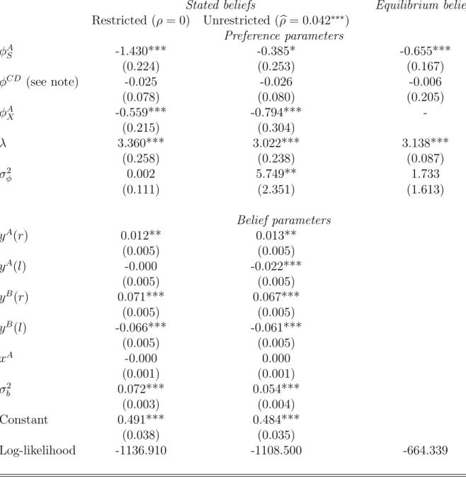
Table 2 presents the results of the restricted and unrestricted versions of the model using stated beliefs. We discuss first the results of the restricted model. We find that
the estimate of ϕAS is -1.430 and highly significant. The estimated magnitude of ϕAS is surprisingly large. It suggests that B players are on average willing to pay up to 1.430
Euros to avoid letting down A players by 1 Euro in treatment S. As argued before the
22Note that we implicitly assume risk neutrality, which implies that we can ignore the players risk
which results from choosing to pay out only a randomly selected subset of games.
23Estimating ϕCD
i (1− b
CD
i ) as a single parameter implicitly assumes that ϕCDi (1− b CD
i ) does not vary across i. We also experimented with a random coefficient specification allowing ϕCDi (1− bCDi ) to vary across i. This did not lead to a signification increase in the log-likelihood function value. We thus report point estimates of ϕCDi (1− bCDi ).
24An extension would be to additionally model possible correlation between beliefs and εn
i. This would allow to control for correlation between decisions and beliefs even in the absence of guilt aversion (see Vanberg (2010) for a discussion).
25Details concerning the log-likelihood function and computation can be found in the appendix of the
estimated value of ϕA
S in the restricted model could be biased upwards due to correlation
between preferences and stated beliefs. Indirect evidence of such a bias can be seen from the estimates of ϕA
X for treatment X. There, correlation between preferences and
beliefs is zero by construction. We find that the estimated value of ϕAX is -0.559 and significant. Furthermore, we reject the null hypothesis that ϕA
S = ϕAX in favor of the
alternative ϕAS < ϕAX (p-value = 0.003). This suggests that WTP estimated in treatment S is significantly higher than the corresponding level estimated in treatment X.
The estimated value of ϕCDi (1−bCDi ) is negative and insignificant, suggesting weak guilt aversion from letting down inactive players. The estimated variance of uϕiA is small and
insignificant. Hence, the restricted model predicts that there is no significant unobserved heterogeneity in guilt aversion across the population. Concerning the parameters in the
belief equations, we find that payoffs enter the equation with the expected signs: B-players state higher probabilities of choosing r when their own payoffs of playing right
yB(r) is higher, and lower probabilities when their payoffs of playing left yB(l) is higher. We also find that B-players state significantly higher probabilities bAi of choosing r when
the payoff of player A increases when choosing r.
We next discuss results of the unrestricted model. First, note that the estimate of ρ
is positive and significant, indicating a significant correlation between guilt aversion and stated beliefs. As we discussed above, a positive and significant estimate of ρ is consistent
with the presence of a consensus effect. Allowing for this correlation has an important impact on our main model estimates. In particular, the estimated value of ϕA
S increases
to -0.385 and is significant against the alternative hypothesis that ϕAS < 0 (p-value =
0.064). On the other hand, the estimated value ϕA
X is -0.794 and remains significant.
Moreover, the estimated value of ϕA
S is no longer significantly different from the estimated
value of ϕA
X (p-value = 0.322) once correlation between preferences and stated beliefs is
accounted for. These results indicate that ignoring the correlation between preferences and stated beliefs in treatment S leads to a upward bias of the estimated level of WTP.
Quantitatively, our model predicts that B players are on average willing between 0.40 and 0.80 Euros to avoid letting down A players by 1 Euro.
The estimated parameters of the belief equation in the unrestricted model are similar
to those of the restricted model. In particular, B players state higher probabilities of choosing r when their payoffs of playing right yB(r) is higher, and lower probabilities
when their payoffs of playing left yB(l) is higher. We also find that B-players state signif-icantly higher probabilities bAi of choosing r when the payoff of player A when choosing
r increases. Hence, it seems that B players think that A players will expect them to
take into account their well being when making their decisions. This finding seemingly
contradicts descriptive evidence presented in Section 3. There, our analysis of the beliefs of A players suggests that A players do not expect that their well-being will be taken into
account by B players. Finally, the estimated value of ϕCDi (1− bCDi ) remains negative and insignificant, suggesting again weak guilt aversion from letting down players C and D.
6
Estimation assuming equilibrium beliefs
In this section we estimate WTP to avoid guilt under the assumption that second-order beliefs are in equilibrium. As we will discuss below, the assumptions underlying the
equilibrium model appear rejected by the data. Hence, purpose of this section is to see whether the equilibrium model can provide reasonable estimates of WTP as a first
approximation.
We do so using only data from treatment S. Estimation of an equilibrium model
using data from treatment S is reasonable given that B players made their decisions in that treatment before knowing that they later had to state their second-order beliefs.
As a result, decisions in treatment S could not have been influenced by the subsequent elicitation of beliefs. We exclude data from treatment X at this point since each B
player in that treatment was provided the first-order beliefs of player A before making his decision. As these first-order beliefs were not restricted to be consistent with the choice
distributions, imposing consistency for estimation of the model parameters in treatment X would almost surely result in a misspecified model.
To estimate the equilibrium model, we use the following specifications of ϕA
ϕAi = ϕAS + uϕiA (9)
ϕCDi = ϕCD+ uϕiCD (10)
where the elements of (9) have been defined previously in (7), ϕCD
i denotes the mean of
ϕCDi , and where uϕiCD is a normally distributed idiosyncratic component with mean zero and variance σ2
ϕ.26 Contrary to (7), we do not estimate a separate value of ϕ for treatment
X as data of the later treatment is not used in the estimation. Under these assumptions, the probability pi(r) that player B will play r in a given game given beliefs (b
A i , b CD i ) is given by pi(r) = ∫ ∫ exp (E(Ui(r))/λ) exp(E(Ui(r))/λ) + exp(E(Ui(l))/λ) hA(uϕiA)hCD(uiϕCD)duϕiAduϕiCD (11)
where the integration is taken over the distributions of uϕiA and uϕiCD and where E(Ui(r))
is given in (8).
To close the model, we assume that beliefs of B players are consistent with the choice
distribution. This restriction implicitly suggests the following assumptions on the infor-mation sets of the players in the game. First, this model assumes that A, C, and D
players know the distributions of ϕAi and ϕCDi . They do not know however the exact val-ues of ϕA
i and ϕCDi of the B player they are matched with. Second, A, C, and D-players
do not know the private component εi(n) of the B player they are matched with, but
they know their population distributions. All other elements of the utility function are
assumed to be known. Hence, A, C and D players can use this information to derive their first-order beliefs concerning the behavior of player B. These first-order beliefs have two
characteristics. First, they are identical across players in the same game (bAi = bCDi ) given all players share the same information set. Second, first-order beliefs will coincide with
the observed distribution pi(r) given in (11). Finally, B-players are assumed to know all
26Hence we assume that the variances of uϕA i and u
ϕCD
i are identical. Allowing these variances to differ does not produce significant increases in the log-likelihood function value (p-value = 0.912).
this, i.e. they know what A, C, and D-players can infer. Hence, they align their
second-order beliefs with the first-second-order beliefs of other players. This generates the following equilibrium restrictions on beliefs
bAi = bCDi = pi(r) for all i = 1, 2, ..., N (12)
Note that these restrictions imply that ϕCD
i can be identified. This differs from the stated
belief model of Section 5 where only the product ϕCDi (1−bCDi ) is identified. Identification of ϕCD
i follows from (8) and the equilibrium restrictions (12) which provide identification
of bCDi . Note also that the equilibrium restrictions on beliefs appear to contradict some of our previous results. In particular, the descriptive evidence in Section 3 suggests that
A players do not expect that B players will take into account the well-being of other
players. On the other hand, estimates of the belief equation in the disequilibrium model
suggest that B-players think that A players will expect them to take into account their well being when making their decisions. Hence, stated second-order beliefs of B players
do not appear in line with the stated first-order beliefs of A players. However, note that these differences do not a priori imply that results of the equilibrium approach will differ
from those of the disequilibrium approach since stated beliefs of A players are not used to estimate any of our models.
To estimate our equilibrium model, let di(r) denote a binary decision variable taking
a value of 1 when player i ∈ {1, 2, ..., N} chooses r, and 0 otherwise. The model log-likelihood is given by QN(θ) = 1 N N ∑ i=1 log [di(r)· pi(r) + (1− di(r))· (1 − pi(r))] (13)
where θ denotes the vector of model parameters. Estimation of θ is done iteratively. In
particular, for a given value of θ, it is simple to solve for the fixed point pi(r) for each
player i. Given these fixed points, we then update θ to maximize (13) given the games {
(yiA(l), yiA(r), yBi (l), yiB(r), yiCD(l), yCDi (r)) : i = 1, 2, ..., N}
As a result, the fixed points are updated iteratively with each new value of θ until equation
Estimates of the equilibrium model are given in the last column of Table 2. We find
that the estimated value of ϕAS is -0.655 and significantly different from zero. Interestingly, the estimated value of ϕA
S is within the range of estimates obtained using the stated belief
model.27 Furthermore, the estimated guilt aversion towards the inactive players ϕCD is small and insignificant. This parallels our findings using the stated belief model and
indicates that we do not loose much by excluding guilt towards inactive players. This result is in line with earlier experimental research documenting the insensitivity towards
inactive players (see e.g. G¨uth and van Damme (1998), Kagel and Wolfe (2001)). Finally, we find that σ2
ϕ is positive but imprecisely measured. This suggests that there is no
unobserved heterogeneity in guilt aversion across the population.
7
Conclusion
This paper has focused on estimating the population level of WTP to avoid guilt using
equilibrium and stated belief models of guilt aversion. Our application focused on a simple game of proposal and response played by a large and representative sample of the Dutch
population.
We found that WTP estimated using stated belief data can be substantially
over-estimated if correlation between stated beliefs and preferences is not accounted for. In particular, the estimated level of WTP in treatment S was found to be significantly greater
(by a factor of 3) than the corresponding level estimated in treatment X. However, we found that the estimated WTP in treatment S was substantially smaller (but remained
significant) when we controlled for this correlation. In fact, controlling for correlation between preferences and beliefs produces estimates of WTP in treatment S which are
insignificantly different from those obtained in treatment X. These result suggest that
27A formal test of the null hypothesis that WTP using exogenously induced beliefs is equal to WTP
in the equilibrium model is complicated by the fact that the equilibrium model uses only data from treatment S (the stated belief models uses data from both treatments) and by the fact that both models are not nested.
ignoring correlation between preferences and beliefs can result in important
overestima-tion of WTP when using stated beliefs. Overall, our range of estimates suggests that responders are on average willing to pay between 0.40 and 0.80 Euro to avoid letting
down proposers by 1 Euro. On the other hand, we fail to find that players are willing to pay to avoid letting down inactive players. This result holds for all models estimated.
Interestingly, replacing stated beliefs by equilibrium restrictions produces estimates of WTP which are significant and fall into the range of estimates obtained when using
ex-ogenously induced beliefs. We interpret this finding as an indication that the equilibrium model provides a good first approximation of the level of WTP in the population even in
one shot games. Future research is needed to investigate whether this result applies to more general models incorporating second-order beliefs (see Dufwenberg and Kirchsteiger,
2004).
Finally, our experimental design shares important similarities with the one used by
Ellingsen, Johannesson, Torsvik and Tjøtta (2009). Like them, we exogenously induced second-order beliefs in our treatment X. Contrary to them however, we find significant
WTP to avoid guilt with exogenously induced second-order beliefs. An interesting di-rection for future research is to examine the factors which can explain this difference.
Socio-economic and cultural differences across subject pools are in principle possible ex-planations. Yet, we found no evidence that guilt aversion varies significantly across
socio-economic dimensions (e.g. age, education, income) which distinguish our representative subject pool from student subject pools. This suggests that cultural (or other
unobserv-able) characteristics can possibly account for the differences in measured guilt aversion across both populations.
A
Technical appendix
We present here the log-likelihood function of the model with stated beliefs. We observe for each player in treatment S a choice and a stated belief. Let ci ∈ {l, r} denote the
choice of player i, and let bAi denote his stated second-order belief concerning the choice of playing r. Finally, define xi ={(yji(r), y
j
i(l)) : j ∈ {A, B, CD}} as the relevant payoff
vector for player i.
Given our model assumptions, it follows that conditional on uϕiA, the likelihood of
observing ( ci, b A i )
is the product of the conditional choice and belief likelihoods
L(ci, b A i |xi, uϕ A i ) = 1 [ci = l] Pr ( ci = l|xi, uϕ A i ) F ( bAi |xi, uϕ A i ) +1 [ci = r] Pr ( ci = r|xi, uϕ A i ) F ( bAi |xi, uϕ A i ) where Pr ( ci = r|xi, uϕ A i ) = exp (E(Ui(r))/λ)
exp (E(Ui(r))/λ) + exp (E(Ui(l))/λ)
Pr ( ci = l|xi, uϕ A i ) = 1− Pr ( ci = r|xi, uϕ A i ) and F ( bAi |xi, uϕ A i ) = Φ ( −x′ iδ+ρu ϕA i 1[y A i (r)<y A i(l)]−ρu ϕA i 1[y A i(r)>y A i (l)] σb ) , if bAi = 0 = f ( bAi−x′iδ+ρu ϕA i 1[yAi(r)<yiA(l)]−ρu ϕA i 1[yiA(r)>yAi(l)] σb ) /σb , if 0 < b A i < 1 = Φ ( 1−x′iδ+ρuϕAi 1[yA i(r)<yAi(l)]−ρu ϕA i 1[yiA(r)>yAi(l)] σb ) , if bAi = 1,
where Φ (·) and f (·) denote respectively the standard normal cumulative and density functions. The likelihood contribution of player i is obtained by integrating out over the distribution of uϕiA L(ci, b A i |xi) = ∫ L(ci, b A i |xi, uϕ A i )h ( uϕiA ) duϕiA (14)
where h (·) denotes the normal density function with mean zero and variance σ2 ϕ. For
players in the treatment X, beliefs are assumed exogenous. Hence, their likelihood con-tribution is simply their conditional choice probability
L(ci|xi) = ∫ L(ci|xi, uϕ A i )h ( uϕiA ) duϕiA (15) = ∫ [ 1 [ci = l] Pr ( ci = l|xi, uϕ A i ) + 1 [ci = r] Pr ( ci = r|xi, uϕ A i )] h ( uϕiA ) duϕiA
The sample log-likelihood is given by
1 N N ∑ i=1 ( log ( L(ci, b A i |xi) ) Ti+ log (L(ci|xi)) [1− Ti] )
where Ti is a dummy variable taking the value of 1 when player i took part in treatment
X, and 0 otherwise. Given no closed form solution exists to this integrals in (14) and (15), a numerical approximation must be performed. In the paper, we approximate the
likelihood contribution by simulation. In particular, we approximate (14) and (15) using the following simulators
eL(ci, b A i |xi) = 1 R R ∑ r=1 L(ci, b A i |xi, uϕ A i,r) eL(ci|xi) = 1 R R ∑ r=1 L(ci|xi, uϕ A i,r) where { uϕi,rA : r = 1, ..., R }
denotes a sequence of R draws taken from the distribution
h
(
uϕiA
)
. Sequences are randomly drawn for each of the N players in the experiment. We use Halton draws to lower the simulation noise of the estimator (see Train (2003) for
Treatment S Treatment X
x y(l) y(r) x y(l) y(r)
Player A 24.935 20.634 20.617 24.648 19.683 21.441 (9.978) (16.750) (16.416) (9.900) (16.778) (16.491) Player B 24.860 22.498 21.511 24.851 24.420 19.904 (7.806) (17.703) (17.138) (8.022) (17.574) (16.964) Player C 25.102 20.782 20.449 25.250 19.920 21.575 (2.194) (16.393) (16.120) (2.039) (16.722) (16.780) Player D 25.102 21.327 21.250 25.250 19.918 21.855 (2.194) (16.683) (16.768) (2.039) (15.826) (16.717)
Table 1: Sample mean and standard deviations of the payoffs of players in treatments S (N = 1078) and X (N = 540). Entries are measured in Euros. The minimum and maximum payoffs for y(l) and y(r) are 0 and 50 Euros respectively for both players and in both treatments. The minimum and maximum payoffs for the outside option x are 10 and 40 Euros for players A and B in both treatments, and 20 and 30 Euros for players C and D in both treatments.
0 .02 .04 .06 .08 Fraction −1 −.5 0 .5 1 Deviation
First−order beliefs of A players
Deviations from observed behavior
0 .02 .04 .06 .08 Fraction −1 −.5 0 .5 1 Deviation
Second−order beliefs of B players
Deviations from observed behavior
Figure 1: Left graph: deviations between stated first-order beliefs of A players and the estimated choice probability of B players (N = 214). Right graph: deviations between the stated second-order beliefs of B players and the estimated expected first-order beliefs of A players (N = 1078).
Stated beliefs Equilibrium beliefs Restricted (ρ = 0) Unrestricted (bρ = 0.042∗∗∗) Preference parameters ϕA S -1.430*** -0.385* -0.655*** (0.224) (0.253) (0.167) ϕCD (see note) -0.025 -0.026 -0.006 (0.078) (0.080) (0.205) ϕAX -0.559*** -0.794*** -(0.215) (0.304) λ 3.360*** 3.022*** 3.138*** (0.258) (0.238) (0.087) σ2 ϕ 0.002 5.749** 1.733 (0.111) (2.351) (1.613) Belief parameters yA(r) 0.012** 0.013** (0.005) (0.005) yA(l) -0.000 -0.022*** (0.005) (0.005) yB(r) 0.071*** 0.067*** (0.005) (0.005) yB(l) -0.066*** -0.061*** (0.005) (0.005) xA -0.000 0.000 (0.001) (0.001) σ2 b 0.072*** 0.054*** (0.003) (0.004) Constant 0.491*** 0.484*** (0.038) (0.035) Log-likelihood -1136.910 -1108.500 -664.339
Table 2: Estimated parameters of the stated and equilibrium belief models. Estimates of the stated belief model (restricted and un-restricted versions) are obtained using decisions and beliefs from treatments S (N =1078) and X (N =540). Estimates of the equilibrium model are obtained using only the decisions in treatment X (N =540). Asymptotic stan-dard errors are in parenthesis. Estimates for the stated belief model presented under the heading ϕCD correspond to estimates of ϕCDi (1− bCDi ). See section 5 for details. ’*’,’**’,’***’ denote significance at the 10%, 5%, and 1% level respectively. Significance of
ϕA
S, ϕAX, and ϕCD are based one one-sided alternatives (eg. ϕAS < 0). Estimates are based
References
Battigalli, P., andM. Dufwenberg (2007): “Guilt in Games,” American Economic
Review Papers and Proceedings, 97, 170–176.
(2009): “Dynamic Psychological Games,” Journal of Economic Theory, 144, 1–35.
Bellemare, C.,and S. Kr¨oger (2007): “On Representative Social Capital,” European
Economic Review, 51, 183–202.
Bellemare, C., S. Kr¨oger, andA. van Soest (2008): “Measuring Inequity Aversion in a Heterogeneous Population using Experimental Decisions and Subjective Probabil-ities,” Econometrica, 76, 815–839.
Charness, G., and M. Dufwenberg (2006): “Promises and Partnerships,”
Econo-metrica, 74, 1579–1601.
Charness, G., and M. Rabin (2005): “Expressed preferences and behavior in experi-mental games,” Games and Economic Behavior, 53, 151–169.
Dawes, R. (1989): “Statistical Criteria for Establishing a Truly False Consensus Effect,”
Journal of Experimental Social Psychology, 25, 1–17.
(1990): “The Potential Nonfalsity of the False Consensus Effect,” in: R. M.
Hogarth (Ed.), Insights in Decision Making: A Tribute to Hillel J. Einhorn.
Dufwenberg, M., and G. Kirchsteiger (2004): “A Theory of Sequential Reci-procity,” Games and Economic Behavior, 47, 268–298.
Ellingsen, T., M. Johannesson, S. T. tta, and G. Torsvik (2009): “Testing Guilt Aversion,” forthcoming, Games and Economic Behavior.
Engelmann, D., and M. Strobel (2000): “The False Consensus Effect Disappears if Representative Information and Monetary Incentives Are Given,” Experimental
Eco-nomics, 3, 241–260.
Falk, A., E. Fehr, and U. Fischbacher (2008): “Testing theories of fairness-Intentions matter,” Games and Economic Behavior, 62, 287–303.
Friedman, D., and D. W. Massaro (1998): “Understanding Variability in Binary and Continuous Choice,” Psychonomic Bulletin and Review, 5, 370–389.
G¨uth, W., and E. van Damme (1998): “Information, Strategic Behavior and Fair-ness in Ultimatum Bargaining - An Experimental Study,” Journal of Mathematical
Harsanyi, J. (1967): “Games with Incomplete Information Played by Bayesian Players, I-III,” Management Science, Theory Series, 14, 159–182, 320–334, 486–502.
Hoffrage, U., S. Lindsey, R. Hertwig, and G. Gigerenzer (2000): “Communi-cating Statistical Information,” Science, 290 (5500), 2261–2262.
Kagel, J., and K. Wolfe (2001): “Tests of Fairness Models Based on Equity Consid-erations in a Three-Person Ultimatum Game,” Experimental Economics, 4, 203–220.
Li, Q.,and J. Racine (2007): Nonparametric Econometrics. Princeton University Press.
Manski, C. F. (2004): “Measuring Expectations,” Econometrica, 72(5), 1329–1376.
Mueller, W., and A. P. de Leon (1996): “Optimal Design of an Experiment in Economics,” The Economic Journal, 106, 122–127.
Ross, L., D. Greene,andP. House (1977): “The false consensus effect: An egocentric bias in social perception and attribution processes,” Journal of Experimental Social
Psychology, 13, 279–301.
Selten, R. (1967): “Die Strategiemethode zur Erforschung des eingeschr¨ankt rationalen Verhaltens im Rahmen eines Oligopolexperiments,” in: H. Sauermann (ed.), Beitr¨age zur experimentellen Wirtschaftsforschung, Vol. I, pp. 136–168.
Sonnemans, J., and T. Offerman (2001): “Is the Quadratic Scoring Rule Really Incentive Compatible?,” Working paper CREED, University of Amsterdam.
Train, K. E. (2003): Discrete Choice Methods with Simulation. Cambridge University Press.
Vanberg, C. (2008): “Why do people keep their promises? An experimental test of two explanations,” Econometrica, 76, 1467–1480.
(2010): “A Short Note of the Rationality of the False Consensus Effect,” Mimeo,