Fabre : Aix Marseille University (Aix Marseille School of Economics, CNRS & EHESS), Château Lafarge, Route
des Milles, 13290 Les Milles Aix-en-Provence, France; tel : 33.4.42.93.59.93 [email protected]
Pallage : ESG UQAM, CIRPÉE and Département des Sciences Économiques, Université du Québec à Montréal, PO
Box 8888 Downtown Station, Montréal, QC, Canada H3C 3P8; tel.1-514 987-3000 ext. 8370; fax : 1 514 987-8494 [email protected]
Zimmermann : Federal Reserve Bank of St. Louis, IZA, RCEA and CESifo, P.O. Box 442, St. Louis, MO
63166-0442, USA; tel. 1 314 444-8647 [email protected]
The views expressed are those of individual authors and do not necessarily reflect official positions of the Federal Reserve Bank of St. Louis, the Federal Reserve System, or the Board of Governors.
The first draft of this paper was written when Fabre was visiting ESG UQAM. Support from AMSE is gratefully acknowledged. The authors thank Steve Ambler, Philippe De Donder, Jean-Denis Garon, and seminar participants at University of Basle, the Swiss National Bank, IZA, the 2013 European Economic Association Meeting in Göteborg, the 2013 Public Economic Theory Meeting in Lisbon and the 2013 Journées Louis-André Gérard-Varet in Aix-en-Provence for useful comments on earlier drafts.
Cahier de recherche/Working Paper 14-27
Universal Basic Income versus Unemployment Insurance
Alice Fabre
Stéphane Pallage Christian Zimmermann
Abstract:
In this paper we compare the welfare effects of unemployment insurance (UI) with an universal basic income (UBI) system in an economy with idiosyncratic shocks to employment. Both policies provide a safety net in the face of idiosyncratic shocks. While the unemployment insurance program should do a better job at protecting the unemployed, it suffers from moral hazard and substantial monitoring costs, which may threaten its usefulness. The universal basic income, which is simpler to manage and immune to moral hazard, may represent an interesting alternative in this context. We work within a dynamic equilibrium model with savings calibrated to the United States for 1990 and 2011, and provide results that show that UI beats UBI for insurance purposes because it is better targeted towards those in need.
Keywords: Universal basic income, Idiosyncratic shocks, Unemployment insurance,
Heterogeneous agents, Moral hazard
Introduction
In recent years, universal basic income policies have been proposed by economists and po-litical scientists as credible alternatives to existing social programs. The idea is simple: Provide citizens with a minimum allowance without means-testing that would give everyone the means to live on a basic level with dignity. A recent example is a constitutional initiative launched in October 2013 in Switzerland.1
Advocates of universal basic income [UBI] can be found all over the political spectrum and in many academic circles, according to the “rainbow coalition” image provided by Anthony Atkinson (Atkinson, 1995). From economists James Meade, Milton Friedman, James Tobin, and Anthony Atkinson to philosophers John Rawls and Philippe Van Parijs, the concept has received much support over the years, for a wide range of reasons: alleviating poverty, simplifying the social protection system, providing additional freedom, etc.
James Meade was one of the first to voice the idea of a social dividend back in 1935 (Meade, 1935, 1989). Juliet Rhys-Williams in the 1940s and then Milton Friedman in the 1960s reintroduced the idea in the form of a negative income tax (Rhys-Williams, 1943; Friedman, 1968), and Tobin offered the concept of a credit income tax (Tobin, 1966; Tobin, Pechman, & Mieszkowski, 1967).2 Friedman’s interest in UBI was motivated by the fact
that free markets did not guarantee that everyone could meet basic needs. Seeking ways for society to correct for this result, he saw efficiency gains in the simplicity of the program. Milton Friedman argued that there were too many problems with existing social programs and that they should be replaced by a unique program, i.e. a negative income tax (Frank, 2006). Rawls (1971) agreed with Friedman on that point.
UBI programs vary in scope according to the perspective of their advocates. While Philippe Van Parijs highlights its universal, unconditional aspect (Van Parijs, 1991),
An-1See, for instance, M¨uller (2013). This debate has contributed to similar questionning in North America
and in Europe (Lowrey, 2013; Van Parijs, 2013, for example).
2Although the UBI policy and the negative income tax can theoretically achieve the same result, there
are slight differences between the two: the negative income tax is distributed at the end of the fiscal year to those capable of filling a tax return. Technically, UBI is paid upfront to all adult members of society. Tobin’s credit income tax is quite close to the negative income tax, yet it may differ in its administration. It inspired the “Demogrant” proposal of the US democratic presidential candidate George McGovern (defeated in 1971 by Richard Nixon). It should be noted Martin Luther King also promoted the idea of a guaranteed income for all Americans to reduce poverty (King, 1967).
thony Atkinson views it rather as a participation income program (Atkinson, 1995). Van Parijs (2000, 2004) thinks of the basic income as a way to provide everyone with the same minimum income, but also as a way to avoid much of the moral hazard of other social pro-grams. For him, UBI certainly reduces poverty, but it is also motivated by ethical reasons: beneath this premise is a sense of social justice and the social reponsibility of a free state for its members. For freedom to be meaningful, a free society must provide everyone with the proper means to exert that freedom (Van Parijs, 1991).3 Herbert Simon also made a state-ment in favor of a UBI policy, praising its justice while highlighting its possible disincentives (Simon, 2000).
Alaska provides one version of basic income, through the Permanent Fund passed in 1976 (Alaska Constitution, Article IX, Section 15), with the very special case of sharing dividends from an Alaskan natural resource, oil. Some field experiments, close to what a basic income could be, were tried in the 1970s in the United States and Canada; see Harris (2005) for a review.
In the economic literature, UBI is sometimes viewed as a way to help the unemployed (Van der Linden, 2002; Lehmann, 2003; Van der Linden, 2004). Dr`eze (1993) shows for instance that a basic income policy could be a good alternative to the reduction of social se-curity contributions (RSSC) if associated with some deregulation of the labor market. There is currently an important debate in Europe on the appropriateness of using UBI as a way to overcome poverty and to replace the existing grant systems (see Vanderborght (2013), for a summary of the political arguments in favor of this system). In a very interesting paper, Van der Linden (2004) uses a dynamic general equilibrium model to analyze the effect of UBI policies on welfare and employment. He shows that the UBI policy reduces the equilib-rium unemployment rate in an environment with risk-neutral agents. The actual comparison between UBI and unemployment insurance [UI] in a framework with self-insurance via sav-ings, moral hazard, and monitoring costs, in the spirit of Friedman’s criticism, has not been investigated.
In this paper, we focus on the welfare comparison between a UBI policy and the
often-3In this sense, basic income can meet the requirement of justice and freedom advocated by Sen (Sen,
1980, 2006, 2009), which implies that people should be given sufficient capabilities to exercise their individual responsibility and choose what they want to do with them. We should note a controversy between Rawls and Van Parijs on the unconditionality of basic income. Although he considers some leisure to be a basic need, Rawls (1993) argued that a social policy should not subsidize those whose life is devoted to leisure. The example used by both authors is that of surfers in Malibu, California.
criticized yet resilient UI. The latter does clearly suffer from several serious flaws, such as tax distortion, the lower savings it generates, moral hazard, and disincentives to work. Designed to offer temporary support to those affected by involuntary unemployment, UI requires important monitoring of beneficiaries. Do they actually look for employment with reasonable effort? Krueger & Mueller (2010) find that the time spent searching is on average a few minutes a day. Do they refuse offers and still try to collect unemployment benefits? Monitoring makes the management of an unemployment insurance program costly. In the state of Oregon, for example, the cost of running the unemployment agency is about $500 per unemployed person per year. This is the type of cost some want to avoid with this simpler policy. Furthermore, since monitoring is never perfect, a proportion of individuals who refuse employment offers manage to go undetected. Moreover, it is common in some countries to disguise quits as lay-offs (Barros, Corseuil, & Foguel, 1999). Hence, the burden of financing an unemployment insurance system can be substantial. This is another type of social cost, which Van Parijs (1991) suggests should matter when comparing the two policies. Clearly, those who contribute most to this burden are workers who may enjoy being rewarded by a basic transfer.
A UBI program is indeed much simpler to manage than a UI program, even if it still generates a tax distortion. Moral hazard, in the sense just described, is not an issue with a basic income policy because workers and unemployed agents receive the same amount. It provides no a priori disincentive to look for work, unless set much too high. It may be socially desirable, therefore, to substitute a properly chosen UBI program for the UI program.4
We test this conjecture within a dynamic model with heterogeneous agents facing em-ployment lotteries and borrowing constraints, which we calibrate to the United States’ labor market dynamics. Our results indicate that, in spite of its many drawbacks, the UI in-stitution is socially very robust to the introduction of a UBI policy. It takes empirically implausible monitoring costs and shirking success probabilities for the optimal basic income policy to dominate the unemployment insurance policy. Also, combining unemployment insurance and universal basic income does not present a socially desirable alternative for reasonable values of our model parameters.
4Another paper that quantitatively investigates the effects of UBI policies is Van der Linden (2002).
The author verifies how UBI affects unemployment in a dynamic general equilibrium model of a unionized economy and shows that some basic income schemes lower the steady-state unemployment rate; in this context, the dynamic adjustment of such reforms can be Pareto-improving.
1
The Model
We work in an environment that mimics the major labor market shocks experienced by both the employed and unemployed. Our model features a job-market lottery `a la Hansen & ˙Imrohoro˘glu (1992) and Pallage & Zimmermann (2001), and a dynamic, discrete-time economy with a continuum of infinitely lived agents of unit measure. These face consumption and labor decisions in the context of borrowing constraints and social policies in the form of a universal basic income and/or an unemployment insurance policy. The model is presented below in a generic way, allowing for all possibilities (UI, UBI, or both).
Model agents are heterogeneous in two important dimensions. At any given time t, they may or may not have a job opportunity and they may have accumulated different amounts of savings to self-insure beyond what the existing policy mix offers against employment shocks.
Employment opportunities occur randomly. Let st∈ {0, 1} denote the result for a specific
agent of the employment lottery at the beginning of period t. It takes value 1 if the agent is offered a job (or the continuation of a job) and value 0 otherwise. The outcomes of the employment lottery follow a Markov process with probabilities p(st|st−1). When observing
that he has the chance to work (st= 1), the agent decides whether or not to accept the offer.
The agent who elects to work is paid an income normalized to 1.
While model agents face a borrowing constraint, they have access to a storage technology that allows them to accumulate assets to smooth consumption against potential future ad-verse employment shocks. We call mt the asset available to the agent at time t. The budget
constraint of an agent in period t can be written as
mt+1+ ct= mt+ ydt, (1)
where ctis the agent’s consumption at time t, mt+1is his future asset, and ydt is his disposable
income. Normalizing an agent’s productivity to 1, we can write the disposable income as one of three possible types depending on the work status and eligibility for unemployment benefits: ytd= (1 − τ )(1 + ω) if he works (1 − τ )(θ + ω) if he collects UI benefits (1 − τ )ω otherwise (2)
agent receives as income replacement from the UI agency, and ω a UBI. The UBI policy is characterized by a constant periodic transfer to all agents.
Eligibility for unemployment benefits is restricted to those agents without a job offer. The unemployment insurance agency’s monitoring of applicants, however, may be imperfect. We model moral hazard by allowing a fraction π of agents who refuse job offers to succeed in fraudulently collecting unemployment benefits.
Unemployment insurance and basic income transfers are financed with a proportional income tax. The endogenous tax rate, τ , is such that the government balances its budget. Unlike the case for basic income, which is given to all, with no questions asked and no strings attached, there is a cost to the provision of unemployment benefits. The necessary – albeit imperfect – monitoring of applicants involves a management cost of the unemployment in-surance agency. Let λ represent the management cost per unemployed per period, regardless of the size of benefits. This cost is taken into account in the government’s budget balancing rule below.
Individual agents have preferences over consumption, ct, and leisure, lt, every period,
which can be represented by the following utility function:
u(ct, lt) =
[c1−σt lσ
t]1−γ − 1
1 − γ , (3)
where γ is the degree of risk aversion of the agent and σ is the elasticity of substitution between consumption and leisure. We assume for simplicity that labor is indivisible, i.e., an agent works either a fixed proportion ¯h of his unit time endowment or does not work at all.
Agents are infinitely lived. They maximize the expected present-value of infinite streams of utility, subject to the above budget constraint:
max E
∞
X
t=0
βtu(ct, lt), (4)
with β ∈ [0, 1), a discount factor.
This problem is recursive and can be written in the form of a Bellman equation (Bellman, 1954), where we drop time subscripts and use prime symbols for future states. The binary decision to work is denoted by x, with x = 1 if a job offer is accepted and 0 otherwise. For an agent with asset m and a job offer (s = 1), the Bellman equation is therefore:
max x ( x max m0 " u((1 − τ )(1 + ω) + m − m0, 1 − ¯h) +X s0 p(s0|1)V (s0, m0) # +(1 − x)(1 − π) max m0 " u((1 − τ )ω + m − m0, 1) +X s0 p(s0|1)V (s0, m0)] # +(1 − x)π max m0 " u((1 − τ )(θ + ω) + m − m0, 1) +X s0 p(s0|1)V (s0, m0)] #) .
For an agent of asset m without a job offer (s = 0), the Bellman equation is:
V (s = 0, m) = max m0 " u((1 − τ )(θ + ω) + m − m0, 1) +X s0 p(s0|0)V (s0, m0)] # .
Once Bellman equations are solved and optimal decision rules extracted, we can construct the distribution of agents f (s, m). We then obtain a series of useful aggregate statistics. The number of workers, for example, is
L =
Z
m
f (1, m)x(1, m)dm. (5)
The number of voluntary unemployed is thus
UV =
Z
m
f (1, m)[1 − x(1, m)]dm. (6)
The number of involuntarily unemployed is simply UI = p(0|1) + p(0|0). Hence the
govern-ment’s budget constraint can be written as
τ [L + ω + θ(πUV + UI)] = ω + θ(πUV + UI) + λ(1 − L). (7)
In the sections to come, we investigate separately the optimal UI policy and the optimal UBI policy for calibrations of the model to the United States at two different time periods. We then turn to the optimal mix of UI and UBI.
2
Solution technique and equilibrium definition
Solving the agents’ problem implies finding, for every possible level of assets and lottery outcome, the optimal labor, consumption, and savings decisions of the agent, as well as the
value function V (s, m). Since there is no closed-form solution for the problem just displayed, we use numerical methods. After properly parametrizing the model, we make use of the fact that the value function is a contraction mapping. Applying Banach’s fixed-point theorem (Kolmogorov & Fomin, 1970), given a policy vector (θ, ω) and a tax rate τ , we iterate on the value function from an arbitrary starting point. This ensures convergence to the unique value function that solves the Bellman equation. We then extract optimal decision rules, given the policy vector, and construct the corresponding stationary distribution of agents, f∗(s, m). We then verify if the government balances its budget for the given tax rate. When needed, we adjust the tax rate and start over until the government budget is balanced.
A steady-state equilibrium in this economy is a choice of labor, consumption, and savings for every individual at every state of the world (s, m); a distribution of agents over states f∗; a policy vector (θ, ω), and a flat tax rate τ , such that (1) all agents maximize their objective function given the policy vector, (2) the distribution of agents is stationary, and (3) the government balances its budget.
When assessing the social desirability of a series of policy vectors, we use a utilitarian social welfare criterion and compare the average value in the steady states corresponding to each policy vector.
3
Parametrization
To conduct numerical simulations, we need to quantify all model parameters to reflect the specific conditions of the United States as closely as possible. We do so for two different time periods: in the 1990s when unemployment risk in the United States was low and in 2011, when unemployment risk was much higher and more persistent in the aftermath of the 2008 crisis and comparable to some European labor markets. This parametrization enables us to compare two policies, unemployment insurance (UI) and universal basic income (UBI), in the context of shocks of very different amplitudes.
We set the length of a period to six weeks, the longest that can accommodate the un-employment durations of the 1990s, as in Hansen & ˙Imrohoro˘glu (1992) and Pallage & Zimmermann (2001), and set the discount factor, β, to 0.995, corresponding to a 4% annual real interest rate.
Table 1: US unemployment statistics
1990 2011
unemployment rate 6% 9%
unemployment duration 12 weeks 36 weeks
Source: Bureau of Labor Statistics (2010-2011)
Table 2: Transition probabilities
1990 p(1|0) p(0|0) p(1|1) p(0|1) 0.5 0.5 0.9892 0.06 2011 p(1|0) p(0|0) p(1|1) p(0|1) 0.1667 0.8333 0.9835 0.0165
the risk aversion parameter, γ, to 2.5 and the elasticity of substitution between consumption and leisure, σ, to 0.67 as in Kydland & Prescott (1982) and Hansen & ˙Imrohoro˘glu (1992).
Since we have normalized a worker’s income to 1, we can interpret all quantitative results in terms of GDP per worker. We consider that an individual works for 45% of his available time when employed, as in Hansen & ˙Imrohoro˘glu (1992). The monitoring costs introduced represent the costs of running the UI agency; while we do not have data for the whole of the United States, we have a reliable figure for Oregon, a state that exhibits features similar to the national US labor market (Pallage & Zimmermann, 2010). The cost of monitoring and administration in that state was $500 per unemployed worker in 2010.5 Based on this figure, we infer a monitoring cost of λ = 0.0048, i.e., the ratio of $500 and the 2010 US GDP per employed person, $104,257 (OECD Economic Outlook, 2010). We assume that the relative monitoring cost is the same in 1990 and 2011.
Shocks in the labor market match the Markov transition probabilities we have computed using the US unemployment rates and unemployment durations provided in Table 1. The probability p(1|0) to exit from unemployment — i.e., to receive an offer if previously without an offer — is the inverse of the average unemployment duration. Using Bayes laws, we can compute the remaining transition probabilities. Table 2 provides the resulting numbers.
4
Quantitative results
We want to compare the socially optimal universal basic income (UBI) and the socially optimal unemployment insurance (UI) in 1990 and in 2011 in terms of average welfare. We do so by comparing steady-state outcomes for various policy parameter values, and we compare their respective effects on welfare, voluntary unemployment, and asset accumulation.
According to our results (Tables 3 and 4), both policies can make individuals better off than a self-insurance mechanism (θ = 0 or ω = 0) and are sustainable at relatively low tax rates.
Table 3 and Figure 1 present the UI results for the 1990 and 2011 United States labor markets, assuming a success rate of shirkers (π) of 20%6 and a monitoring cost, λ, of 0.0048
per unemployed person. Based on the average utility of agents in our model of the 2011 labor market, the optimal replacement ratio in the UI policy is 25%. This number is not far from the observed coverage once you take into account eligibility requirements. As is standard in this literature, as the replacement ratio θ increases, average assets diminish and the number of voluntarily unemployed (shirkers) rises. The optimal replacement rate is higher in 2011 than in 1990, reflecting the higher riskiness of the 2011 labor market (higher unemployment rate and average unemployment duration). This also implies a stronger tendency for agents to accumulate assets in the steady state. Average welfare is clearly higher in the less risky 1990 economy.
Table 4 and Figure 2 are the UBI counterparts to Table 3 and Figure 1. Moral hazard is no longer relevant as every agent in the economy is eligible for UBI benefits whether employed or unemployed; consequently there is no need to monitor agents and, hence, the monitoring cost is zero. Our results indicate that the average welfare is maximized in 1990 and 2011 for UBI allowances of, respectively, 1.25% and 2.25% of a worker’s usual labor income. A UBI program is clearly sustainable, but its socially optimal form implies very small transfers that are equivalent to a yearly supplement of about $2,000 in 2011, before tax. We do not observe large numbers of agents quitting employment in the neighborhood of the optimal UBI policy. But quitters quickly become a problem as the UBI transfer is increased. For a 5% income supplement, for instance, the voluntary unemployment rate would be close to 4%
6It is commonly agreed that 20% is a reasonable number for π, the proportion of agents refusing job offers
who nevertheless manage to collect UI benefits (Pallage & Zimmermann, 2005). We provide results for other levels of shirking success in Table 5.
under both the 1990 and 2011 calibrations. Of course, with fewer agents employed, the tax rate required to sustain the policy becomes rapidly large and induces more quitting behavior. Unlike in Van der Linden (2004), the UBI policy thus raises the actual unemployment rate. The likelihood of quitting rises exponentially in response to increases in UBI benefits.7 This
explains why the socially optimal UBI policy cannot be very generous.
We now want to compare both policies. As previously noted, both UI and UBI programs are significant improvements over the laissez-faire, i.e., self-insurance shown in the first lines of Tables 3 and 4. The UBI policy around its optimum may appear as a credible alternative to UI in both periods. However, for the shirking success probability considered in Table 3 (π = 0.20) and the monitoring cost calibrated to Oregon, the optimal UI policy is socially more desirable, as a comparison of average welfare across Tables 3 and 4 suggests. For both calibrations, UI is clearly a better insurance mechanism against idiosyncratic employment shocks than UBI, and the inefficiency caused by monitoring costs and cheating behavior do not offset this fact in our simulations. In fact, for society to switch from UI to UBI would require a transfer corresponding to 0.02% and 0.18% of consumption in 1990 and 2011, respectively.8 Given the small benefits, such small consumption equivalence numbers should not be surprising. Indeed, self-insurance can at least partially offset what either of the policies does not offer through its lack of generosity. Figure 3 gives a good idea of the respective impacts of UI and UBI on all variables in the 2011 calibration. A similar figure could be produced for the 1990 calibration with somewhat smaller effects.
Why doesn’t UBI measure up to UI? While proponents of the UBI policy stress the insurance factor and the reduced administrative and monitoring cost, the main argument against it has always been that it could significantly reduce the labor supply. We find that this latter effect is very strong, to the point that UBI in the optimal results barely provides any transfer and thus provides little insurance. UI is socially preferred because it does provide insurance — that is, a conditional transfer — and transfers are not “wasted” on people who do not need them (employed workers). Moral hazard under UI does not seem to be enough of a problem to overturn this in our calibrations of the US labor market in 1990 and 2011.
7Quitting is not necessarily bad for well-being, as quitters enjoy leisure, but it drives up the tax rate very
fast.
8The transfer is computed as the increase in consumption at all states needed to equate the average value
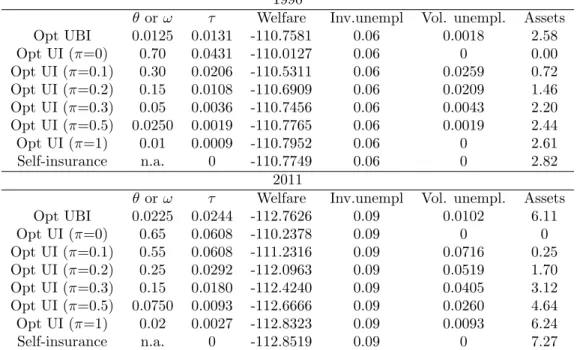
Of course, it is a standard result in the optimal unemployment insurance literature—as visible in Table 5—that increased moral hazard drives down the optimal replacement rate. Similar results were reported by Hansen & ˙Imrohoro˘glu (1992), Wang & Williamson (1996, 2002), Hopenhayn & Nicolini (1997), and Pallage & Zimmermann (2001). We show here that society, on average, does dislike moral hazard, but not as much as the implicit free riding that comes with UBI in our model economies.9 In fact, it would take shirking success
probabilities or monitoring costs substantially larger than our base scenario in Table 3 for UBI to be socially preferred to UI. Table 5 shows that moral hazard needs to be quite high in both economies for society to favor UBI (more than 50% of shirkers succeeding in collecting UI benefits in 2011 and 30% in 1990). Similarly, setting shirking success at π = 0.20, Table 6 shows that for monitoring costs in the neighborhood of that calibrated from Oregon, UI dominates UBI in terms of the average welfare it provides. The table also shows how monitoring costs affect the average well-being and the degree of optimal UI generosity, as measured by the replacement ratio θ. We restrict ourselves in Table 6 to reasonable values of monitoring costs and illustrate their impact on average utility. As we increase monitoring costs beyond those values, however, we eventually reach a level in which UBI starts dominating UI on the social preference scale.
In the space of shirking success π and monitoring costs λ, Figure 4 provides society’s indifference frontiers between both polices for the job market calibrations of 1990 and 2011. For every point east of either frontier, UBI is socially preferred to UI for the relevant period. The higher riskiness of labor markets in 2011 pushes the indifference frontier to the east of that in 1990. For every level of shirking success, society in 2011 is willing to tolerate higher monitoring costs to keep its unemployment insurance or, alternatively, for given monitoring costs, society is willing to tolerate higher levels of shirking success. The switch to UBI requires more extreme values of shirking success or monitoring costs than in 1990.
We also tested whether a combination of UI and UBI would be socially preferred. It turns out that the optimal combination of both policies implies UBI transfers of zero. Figure 5 illustrates this for the 2011 calibration. The universal basic income makes it easier for agents to shirk. In an economy with moral hazard and idiosyncratic shocks, shirking is costly as it imposes a higher tax burden on those who finance the social policy. The addition of a UBI
9Interestingly, moral hazard is less detrimental for the UI system with large shocks (2011 case) than with
small shocks (1990 case). With large shocks, a UI system is always preferred to a self-insurance system, even with high moral hazard (see Table 5); with smaller shocks, it is not that definite.
component to a UI policy thus never improves average welfare for reasonable values of the parameters. One way to think of why UI so clearly dominates UBI is that UI is simply better at targeting support where it is needed most. UBI has the major disadvantage of requiring much higher (distorting) taxes to sustain the same level of support for the needy, while wasting most of its payments on those with low marginal utility of consumption. Clearly UBI, even if it is sustainable for the economy, is not a good insurance mechanism against shocks.
The model economy we consider here is obviously a very crude approximation and could benefit from some bells and whistles. We want to argue that such additions are not necessary, as they would only reinforce our results that UI generally dominates UBI. For example, suppose we add heterogeneity with regard to the employment lottery: some have lower employability as is typical for lower-skilled workers. These would prefer the targeted help from UI. The most-skilled workers would prefer UI as well, as they do not need the income support from UBI (low marginal utility of consumption) and would reduce their labor supply due to the distorting taxes. Just as in the benchmark case we presented, UBI would end up contributing very little. UBI would help those who cannot work at all. But it is easy to argue that they would be better helped with a program specifically addressing this inability to work, as is the case in many countries.
One could also argue that our UI policy is oversimplified. For example, almost every UI system in the world has a finite eligibility period or a cap for unemployment generosity. Even when unemployed, one has to satisfy some additional criteria to qualify. And the level of benefits is often adjustable to the needs of the claimant, such as the family situation or capacity to overcome an unemployment spell, through the means of an asset test. Adding all these features would enhance the targeting ability of UI and thus increase its advantage over UBI.
We should note that in countries in which it is difficult for the unemployment agency to distinguish between quits and lay-offs, moral hazard is likely much higher than in the base scenario considered here for the United States. In such case, the relevant value for π is closer to 1. As Figure 4 shows, UBI may dominate UI policies in such a scenario. A relevant example may be Brazil according to Barros et al. (1999).
5
Conclusion
In this paper, we provide a quantitative comparison of an optimal universal basic income policy and an optimal unemployment insurance program in an economy with idiosyncratic shocks. While an unemployment insurance program is better equipped to respond to em-ployment shocks, it suffers from moral hazard and is costly to manage. Monitoring costs are not trivial and add to the social cost of administering the policy. So does moral hazard, by allowing a fraction of agents to abuse the unemployment insurance program. A universal basic income policy, however, has no such social costs and is very simple to manage.
We test the conjecture that a universal basic income may, under moral hazard and in the presence of monitoring costs, perform better. We conduct a wide variety of experiments and compare the social desirability of these policies.
Our results show that an optimal UBI is feasible. Nevertheless, the UI policy is socially robust to the introduction of UBI in the presence of idiosyncratic shocks. It takes empirically implausible monitoring costs and shirking success probabilities for the optimal basic income policy to dominate in terms of welfare the unemployment insurance policy in the economy calibrated to the 2011 United States labor market. With idiosyncratic shocks of smaller amplitude (such as those characterizing the 1990 US labor market dynamics), UBI may represent a more reasonable alternative, even if the UI policy remains socially preferred.
The superiority of UI is anchored in its ability to help those who are most in need. Even a very crude UI system with no asset tests and indefinite eligibility is able to easily beat UBI, which distributes funds blindly and must be financed through distortionary taxation.
Of course, this paper limits the study of universal basic income to its comparison with a UI policy in a particular model. It does not claim to have the last word on UBI systems. Other paths could be explored. We could consider different skills among the population; in this case we have argued that UBI is likely to reinforce the dominance of UI. One could study the impact of transitions. Indeed, we have only compared steady states so far. Transitions can induce large costs in the short-term that can outweigh long-term advantages. Given that the status quo in industrialized countries is typically a UI policy, it is very unlikely that a transition to UBI would prove to be beneficial overall.
References
Atkinson, A. B. (1995). Public Economics in Action: The Basic Income/Flat Tax Proposal. Clarendon Press, Oxford. Barros, R. P., Corseuil, C. H., & Foguel, M. (1999). Os incentivos adversos dos programas de seguro-desemprego e do FGTS
no Brasil. Mimeo, IPEA, Rio de Janeiro, Brazil.
Bellman, R. (1954). The theory of dynamic programming. Bulletin of the American Mathematical Society, 60, 503–516. Dr`eze, J. H. (1993). Can varying social insurance contributions improve labour market efficiency?. In Atkinson, A. B. (Ed.),
Alternatives to Capitalism: The Economics of Partnership. MacMillan, London.
Frank, R. H. (2006). The other Milton Friedman: a conservative with a social welfare program. The New York Times. November 23.
Friedman, M. (1968). The case for a negative income tax. In Laird, M. R. (Ed.), Republican Papers, pp. 202–220. Anchor, Garden City, NY.
Hansen, G. D. & ˙Imrohoro˘glu, A. (1992). The role of unemployment insurance in an economy with liquidity constraints and moral hazard. Journal of Political Economy, 100 (1), 118–142.
Harris, R. (2005). The guaranteed income movement of the 1960s and 1970s. In Widerquist, K., Lewis, M., & Pressman, S. (Eds.), The Ethics and Economics of the Basic Income Guarantee, pp. 77–94. Ashgate Publishing, Hampshire UK and Burlington VT.
Hopenhayn, H. A. & Nicolini, J. (1997). Optimal unemployment insurance. Journal of Political Economy, 105 (2), 412–438. King, M. L. J. (1967). Where Do We Go from Here: Chaos or Community? Harper and Row, New York, NY.
Kolmogorov, A. & Fomin, S. (1970). Introductory Real Analysis. Dover, Mineola, NY.
Krueger, A. B. & Mueller, A. (2010). Job search and unemployment insurance: new evidence from time use data. Journal of Public Economics, 94 (3-4), 298–307.
Kydland, F. E. & Prescott, E. C. (1982). Time to build and aggregate fluctuations. Econometrica, 50 (6), 1345–1370. Lehmann, E. (2003). Evaluation de la mise en place d’un syst`´ eme d’allocation universelle en pr´esence de qualifications
h´et´erog`enes : le rˆole institutionnel du salaire minimum. ´Economie et Pr´evision, 157 (1), 31–50.
Lowrey, A. (2013). Switzerland’s proposal to pay people for being alive. The New York Times Magazine. November 12. Meade, J. E. (1935). Outline of an economic policy for a labour government. In Howson, S. (Ed.), The Collected Papers of
James Meade. Volume I: Employment and Inflation. Unwin Hyman Ltd, 1988, London.
Meade, J. E. (1989). Agathotopia: The Economics of Partnership. Aberdeen University Press, Aberdeen.
M¨uller, J. (2013). D´ebat sur le revenu de base: lib´eration de la Suisse ou attaque contre l’Etat social. Revue Suisse, pp. 17–18. Pallage, S. & Zimmermann, C. (2001). Voting on unemployment insurance. International Economic Review, 42 (4), 903–924. Pallage, S. & Zimmermann, C. (2005). Heterogeneous labor markets and the generosity towards the unemployed: an
interna-tional perspective. Journal of Comparative Economics, 33, 88–106.
Pallage, S. & Zimmermann, C. (2010). Unemployment Accounts: A Better Way to Protect the Unemployed. Cascade Policy Institute, Portland, Oregon.
Rawls, J. (1971). A Theory of Justice. Harvard University Press, Cambridge, MA. Rawls, J. (1993). Political Liberalism. Columbia University Press, New York, NY. Rhys-Williams, J. (1943). Something to look forward to. MacDonald, London.
Sen, A. K. (1980). Equality of what?. In McMurrin, S. (Ed.), The Tanner Lectures on Human Values, Vol. 1. University of Utah Press.
Sen, A. K. (2009). The Idea of Justice. Harvard University Press, Cambridge. MA. Simon, H. A. (2000). Ubi and the flat tax. Boston Review.
Tobin, J. (1966). The case of an income guarantee. The Public Interest, 4, 31–41.
Tobin, J., Pechman, J. A., & Mieszkowski, P. M. (1967). Is a negative income tax practical?. The Yale Law Journal, 77 (1), 1–27.
Van der Linden, B. (2002). Is basic income a cure for unemployment in unionized economies? a general equilibrium analysis. Annales d’´economie et de statistique, 66, 81–105.
Van der Linden, B. (2004). Active citizen’s income, unconditional income and participation under imperfect competition: a welfare analysis. Oxford Economic Papers, 56 (1), 98–117.
Van Parijs, P. (1991). Why surfers should be fed: the liberal case for an unconditional basic income. Philosophy & Public Affairs, 20 (2), 101–131.
Van Parijs, P. (2000). A basic income for all. Boston Review, 25 (5), 4–8.
Van Parijs, P. (2004). Basic income: a simple and powerful idea for the twenty-first century. Politics and Society, 32 (1), 7–39. Van Parijs, P. (2013). Pour la mise en place d’un revenu universel. Le Monde. 13 d´ecembre.
Vanderborght, Y. (2013). Basic income, social justice and poverty. In Sciurba, A. (Ed.), Trends in Social Cohesion #25: Redefining and Combating Poverty: Human Rights, Democracy and Common Goods in Today’s Europe, pp. 267–283. Council of Europe Publishing, Strasbourg.
Wang, C. & Williamson, S. (1996). Unemployment insurance with moral hazard in a dynamic economy. Carnegie-Rochester Conference Series on Public Policy, 44, 1–41.
Table 3: UI with π=0.2 and λ=0.0048
1990
θ τ Welfare Inv.unempl Vol.unempl. Assets
0 0 -110.7749 0.06 0.0000 2.82 0.05 0.0035 -110.7328 0.06 0 2.20 0.10 0.0070 -110.6931 0.06 0.0091 1.80 0.15* 0.0108 -110.6909 0.06 0.0209 1.46 0.20 0.0151 -110.7360 0.06 0.0352 1.16 0.25 0.0200 -110.8332 0.06 0.0518 0.91 0.30 0.0256 -110.9870 0.06 0.0697 0.68 0.35 0.0318 -111.1998 0.06 0.0890 0.50 0.40 0.0386 -111.4552 0.06 0.1077 0.36 2011
θ τ Welfare Inv.unempl Vol.unempl. Assets
0 0 -112.8519 0.09 0.0000 7.27 0.05 0.0054 -112.6159 0.09 0.0023 5.31 0.10 0.0107 -112.3922 0.09 0.0111 4.12 0.15 0.0163 -112.2290 0.09 0.0226 3.16 0.20 0.0225 -112.1350 0.09 0.0370 2.36 0.25* 0.0292 -112.0963 0.09 0.0519 1.70 0.30 0.0366 -112.1332 0.09 0.0689 1.16 0.35 0.0449 -112.2727 0.09 0.0887 0.72 0.40 0.0541 -112.4968 0.09 0.1097 0.39
Note: In the table, average welfare is computed as the weighted sum of households’ value function at the steady state corresponding to the given UI policy. The tax rate presented guarantees a balanced budget for the chosen policy. The socially optimal UI replacement ratio, θ, is identified with a?. All statistics are aggregated from equilibrium households’ decisions.
Table 4: Universal Basic Income
1990
ω τ Welfare Inv.unempl Vol.unempl. Assets
0 0 -110.7749 0.06 0.0000 2.82 0.01 0.0105 -110.7585 0.06 0.0000 2.61 0.0125* 0.0131 -110.7581 0.06 0.0018 2.58 0.0150 0.0158 -110.7596 0.06 0.0039 2.55 0.0175 0.0184 -110.7629 0.06 0.0064 2.52 0.02 0.0210 -110.7647 0.06 0.0077 2.49 0.03 0.0315 -110.7921 0.06 0.0168 2.37 0.05 0.0526 -110.9219 0.06 0.0396 2.15 0.10 0.1073 -111.7223 0.06 0.1078 1.68 0.20 0.2249 -115.6647 0.06 0.2507 1.00 0.30 0.3569 -124.6774 0.06 0.3994 0.53 2011
ω τ Welfare Inv.unempl Vol.unempl. Assets
0 0 -112.8519 0.09 0.0000 7.2739 0.01 0.0109 -112.7925 0.09 0.0022 6.59 0.0125 0.0136 -112.7834 0.09 0.0035 6.49 0.0150 0.0163 -112.7774 0.09 0.0057 6.39 0.0175 0.0190 -112.7705 0.09 0.0066 6.29 0.02 0.0217 -112.7689 0.09 0.0093 6.20 0.0225* 0.0244 -112.7626 0.09 0.0102 6.11 0.0250 0.0271 -112.7669 0.09 0.0134 6.02 0.0275 0.0298 -112.7633 0.09 0.0143 5.93 0.03 0.0325 -112.7714 0.09 0.0179 5.84 0.05 0.0541 -112.8397 0.09 0.0360 5.21 0.10 0.1100 -113.5896 0.09 0.1011 3.90 0.20 0.2305 -117.7240 0.09 0.2422 2.08 0.30 0.3639 -126.9929 0.09 0.3856 0.95
Note: In the table, average welfare is computed as the weighted sum of households’ value function at the steady state corresponding to the given UBI policy. The tax rate presented guarantees a balanced budget for the chosen policy. The socially optimal UBI, ω, is identified with a?. All statistics are aggregated from equilibrium households’ decisions.
Figure 3:
Table 5: Policy comparisons for different levels of shirking success, with λ = 0.0048
1990
θ or ω τ Welfare Inv.unempl Vol. unempl. Assets Opt UBI 0.0125 0.0131 -110.7581 0.06 0.0018 2.58 Opt UI (π=0) 0.70 0.0431 -110.0127 0.06 0 0.00 Opt UI (π=0.1) 0.30 0.0206 -110.5311 0.06 0.0259 0.72 Opt UI (π=0.2) 0.15 0.0108 -110.6909 0.06 0.0209 1.46 Opt UI (π=0.3) 0.05 0.0036 -110.7456 0.06 0.0043 2.20 Opt UI (π=0.5) 0.0250 0.0019 -110.7765 0.06 0.0019 2.44 Opt UI (π=1) 0.01 0.0009 -110.7952 0.06 0 2.61 Self-insurance n.a. 0 -110.7749 0.06 0 2.82 2011
θ or ω τ Welfare Inv.unempl Vol. unempl. Assets Opt UBI 0.0225 0.0244 -112.7626 0.09 0.0102 6.11 Opt UI (π=0) 0.65 0.0608 -110.2378 0.09 0 0 Opt UI (π=0.1) 0.55 0.0608 -111.2316 0.09 0.0716 0.25 Opt UI (π=0.2) 0.25 0.0292 -112.0963 0.09 0.0519 1.70 Opt UI (π=0.3) 0.15 0.0180 -112.4240 0.09 0.0405 3.12 Opt UI (π=0.5) 0.0750 0.0093 -112.6666 0.09 0.0260 4.64 Opt UI (π=1) 0.02 0.0027 -112.8323 0.09 0.0093 6.24 Self-insurance n.a. 0 -112.8519 0.09 0 7.27
Table 6: Policy comparisons for different levels of monitoring costs with π=0.20
1990
θ or ω τ Welfare Inv.unempl Vol. unempl. Assets Opt UBI 0.0125 0.0131 -110.7581 0.06 0.0018 2.58 Opt UI (λ=0) 0.15 0.0104 -110.6402 0.06 0.0209 1.46 Opt UI (λ=0.001) 0.15 0.0105 -110.6529 0.06 0.0209 1.46 Opt UI (λ=0.0048) 0.15 0.0108 -110.6909 0.06 0.0209 1.46 Opt UI (λ=0.01) 0.10 0.0073 -110.7393 0.06 0.0091 1.20 Self-insurance n.a. 0 -110.7749 0.06 0 2.82 2011
θ or ω τ Welfare Inv.unempl Vol. unempl. Assets Opt UBI 0.0225 0.0244 -112.7626 0.09 0.0102 6.11 Opt UI (λ=0) 0.25 0.0284 -112.0027 0.09 0.0521 1.70 Opt UI (λ=0.001) 0.25 0.0286 -112.0226 0.09 0.0521 1.70 Opt UI (λ=0.0048) 0.25 0.0292 -112.0963 0.09 0.0519 1.70 Opt UI (λ=0.01) 0.25 0.0300 -112.1992 0.09 0.0517 1.70 Self-insurance n.a. 0 -112.8519 0.09 0 7.27