Using a Jiles-Atherton vector hysteresis model for isotropic magnetic materials with the FEM, Newton-Raphson method and relaxation procedure
Texte intégral
Figure

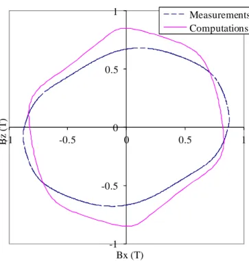
![Figure 4 shows the b ax h sx - and b ay h sy -loops obtained at point 1. The appearance is almost the same as the loops of figure 14 of [3]](https://thumb-eu.123doks.com/thumbv2/123doknet/5631113.136000/15.892.184.702.240.805/figure-shows-loops-obtained-point-appearance-loops-figure.webp)
Documents relatifs
In the present paper, a microsphere model taking into account rate-independent hysteresis is proposed and applied to model filled silicone rubbers behavior.. The hysteresis model
In magnetization processes, these independent contributions cannot evidently be found at the level of single spins, and neither a t the one of single Bloch walls ,
The corresponding solution method by use of the finite element method FEM is called FE2 , since FE analyses have to be carried out to solve the microscopic BVPs with input data of
Dynamic magnetic scalar hysteresis lump model, based on Jiles-Atherton quasi- static hysteresis model extended with dynamic fractional derivatives.. INTERMAG 2018 – GT 05 – 27/04/2018
In the case of magneto-elastic behaviour, the equivalent stress for a given multiaxial loading σ is defined as the uniaxial stress σ eq - applied in the direction parallel to
∆E effect for an iron-cobalt alloy: longitudinal and transverse magnetostriction strain as a function of the applied stress σ, modeling (line) and experimental (points) results.
Abstract— The aims of this work is the modeling of the hysteresis loop in ferromagnetic materials, and allowed to highlight of the difficulty that exists in the choice of an model,
2014 A brief survey is made of some of the problems involved in the development of experimental methods of obtaining information on the domain processes involved in
