This is an author-deposited version published in:
http://oatao.univ-toulouse.fr/
Eprints ID: 5305
To link to this article: DOI: 10.1504/EJIE.2011.042742
http://dx.doi.org/10.1504/EJIE.2011.042742
To cite this version:
Haït, Alain and Artigues, Christian An hybrid
CP/MILP method for scheduling with energy costs. (2011) European
Journal of Industrial Engineering, 5 (4). pp. 471-489. ISSN 1751-5254
O
pen
A
rchive
T
oulouse
A
rchive
O
uverte (
OATAO
)
OATAO is an open access repository that collects the work of Toulouse researchers and
makes it freely available over the web where possible.
Any correspondence concerning this service should be sent to the repository
administrator:
[email protected]
An hybrid CP/MILP method for scheduling
with energy costs
Abstract: This paper deals with energy-related job scheduling for a foundry, in order to minimize the electricity bill. Accounting for energy and human resource constraints leads to better solutions in terms of cost and overall energy consumption. We propose a hybrid heuristic based on a two-step constraint/mathematical programming approach that improves significantly the computation time, compared to the full MILP model.
Keywords: Scheduling, Energy, Human resources, Parallel machines, Hybrid approach.
1 Introduction
The problem of energy consumption in industry exists for several decades, but has become much more critical in the beginning of this century. The main reasons are demand increase with the industrialization of China and India, inducing higher prices, and environmental aspects (reliance on fossil energy, global warming). The reflexion about a better energy consumption is a real challenge now and for the future.
Consequently, energy consumption is a matter of concern in the industrial sector. Long range solutions are about alternative sources of energy and design of new types of industrial networks (Gibbs and Deutz, 2007). Waiting for these solutions to be effective, shorter-range responses can be found for industry. Integration of the energy aspects into production guarantees a better use of energy (Cheung and Hui, 2004). For example, the use of co generation, along with a coordination of product and energy operations is a promising issue in the process industry (Agha et al., 2008, 2009; Korhonen, 2002).
These new constraints force to reconsider production planning and scheduling models. From a scheduling point of view, accounting for energy, and more generally utilities or secondary resources involve changes due to the availability of these re-sources, their cost or their impact on the duration of the operations. In this paper, we present an example of scheduling for a foundry, with electricity costs, accounting for energy and human resource constraints. Next section presents informally the problem and the related work. Section 3 presents the mathematical model, and in section 4 we propose a constraint/mathematical programming heuristic to solve efficiently the problem. Section 5 shows some experimental results.
2 Problem statement
The addressed problem comes from a pipe-manufacturing plant, presented in Ha¨ıt et al. (2007), and more precisely, the foundry where metal is melted in induc-tion furnaces and then cast in individual billets.
The foundry has five lines of production (furnaces). Each melting operation has to be assigned to a furnace and scheduled within a time window. Furthermore, it has a variable duration that depends on the power given to the furnace (constrained by physical and operational considerations). A melting job is thus composed of three sequential parts (Fig. 1): loading, heating and unloading. Each furnace has un-availability periods representing operator temporary operator unun-availability. While heating can be performed during an unavailability period, loading and unloading operations need the presence of an operator. The durations of loading and un-loading are known (Dl and Du), but heating duration depends on the following
conditions:
• melting duration depends on the power given to the furnace, in a range [Pmin, Pmax]. Melting of job j ends when an amount Ej of energy has been
supplied.
• when melting is complete, the temperature must be hold in the furnace until an operator is ready to unload it. To this aim, power Phold is applied to the
furnace.
Furnace
t
load. heating unload.
tl tm th tu
Dl Melting Holding Du
load. unavailable unload. Operator
t
Figure 1 Job description and corresponding operator’s tasks.
The goal is to minimize the cost of the schedule, depending on the energy con-sumed and on penalties when the overall power in the foundry exceeds a given subscribed value. The energy consumption is recorded and the power is evaluated every 15’ interval by the electricity provider, using a counter.
From a scheduling view-point, this facility can easily be recognized as a parallel machine problem. Parallel machine scheduling without energy considerations has been widely studied (Chen and Sin, 1990), specially because it appears as a re-laxation of more complex shop or project scheduling problems like the hybrid flow shop scheduling problem or the resource-constrained project scheduling problem. Several methods have been proposed to solve this problem. In Chen and Powell (1999), a column generation strategy is proposed. Pearn et al. (2007) propose a linear program and an efficient heuristic for solving large-size instances of a priority constraints and family setup times problem. Salem et al. (2000) solve the problem
local search methods for a parallel machine scheduling problem with precedence constraints and sequence-dependent setup times. Neron et al. (2008) compare two different branching schemes and several tree search strategies for the problem with release dates and tails for the makespan minimization case. In Baptiste et al. (2000), a constraint programming-based approach is proposed to solve the weighted number of late jobs problem. In Sadykov and Wosley (2006), An hybrid Integer/Constraint Programming approach is propose to solve a minimum-cost assignment problem. Among the variants presented in the latter, the most effective strategy is to com-bine a tight and compact, but approximate, mixed integer programming (MIP) formulation with a global constraint testing single machine feasibility.
Energy consumption management is a critical issue in computer systems, net-works and embbeded systems where many (online) algorithmic problems are raised and well studied Irani and Pruhs (2005). On the other hand, these considerations are recent in production. Production scheduling for steel manufacturing has been studied, but few papers focus on energy cost (Nolde and Morari, 2010). Complexity is a major difficulty for the integration of energy constraints to production schedul-ing (Sec. 3.5) and the literature on the subject is rather sparse. This generally leads to develop heuristics. For example, Boukas et al. (1990) propose a hierarchi-cal approach for scheduling a steel plant subject to a global limitation on the power supplied to the furnaces. Harjunkoski and Grossmann (2001) use a decomposition approach to solve a steel manufacturing scheduling problem with multiple products.
3 Mathematical programming model
In this section, we propose a continuous-time MILP model of the addressed problem. Then this model will be included in a two-level heuristic presented in the next section.
3.1 Scheduling model
Jobs are defined by the operation start times tl (loading), tm (melting, tm =
tl+ Dl), th (holding) and tu (unloading). These times are continuous variables in
the model. Job assignment and sequencing are represented by the following binary variables (the nomenclature is given in Appendix A):
• x(f, j) = 1 if furnace f is allocated to job j, 0 otherwise; • y(j1, j2) = 1 if job j1 precedes job j2, 0 otherwise.
The assignment and sequencing constraints are: X f ∈F x(f, j) = 1 ∀j ∈ J (1) y(j1, j2) + y(j2, j1) ≤ 1 ∀(j1, j2) ∈ J2, j16= j2 (2) y(j1, j2) + y(j2, j1) ≥ x(f, j1) + x(f, j2) − 1 ∀f ∈ F, (j1, j2) ∈ J2, j16= j2 (3)
Equation (1) indicates that exactly one furnace is allocated to a job, while (2) represents the antisymmetry of the precedence relation. Finally, (3) ensures that if the same furnace is allocated to two jobs, one precedes the other.
The operation start times depend on release and due dates, operation sequence and precedence constraints:
tl(j) ≥ Rel(j) ∀j ∈ J (4) tm(j) = tl(j) + Dl(j) ∀j ∈ J (5) th(j) ≥ tm(j) + E(j)/Pmax ∀j ∈ J (6) th(j) ≤ tm(j) + E(j)/Pmin ∀j ∈ J (7) tu(j) ≥ th(j) ∀j ∈ J (8) tu(j) ≤ Due(j) − Du(j) ∀j ∈ J (9) tl(j2) ≥ tu(j1) + Du(j1) − M (1−y(j1, j2)) ∀(j1, j2) ∈ J2, j16= j2 (10)
Constraints (5)-(8) set the sequence of operation start times for job j: first tl,
then tm, thand finally tu(Fig. 1). Note that (6) and (7) use the min/max durations
of job j. Constraints (4) and (9) situate job j in the range [Release date; Due date] and job sequencing is given by (10) according to the precedence variables y(j1, j2).
The ‘Big-M’ value in (10) is set to the horizon length.
3.2 Heating operation logic
The time horizon is divided into Imax intervals of uniform duration D. These
intervals will be used to measure the consumption of energy and then to estimate the instantaneous power as the mean power on each interval.
3.2.1 Time/interval binary variables.
During the melting of job j, an amount of energy em(j, i) is supplied at an
interval i. It is the integration of the power given to the furnace over the melting duration dm(j, i) in this interval. Our model uses energy and duration as variables,
but it is not necessary to represent explicitly the power, considered as a constant over the melting duration for each interval (Fig. 2). During the holding phase (waiting for an operator to unload the furnace), the power is set to Phold. The
holding duration of job j at interval i is given by the variable dh(j, i). Melting and
holding of a job may appear in the same interval when th belongs to this interval
(e.g. interval 3 in Fig. 2).
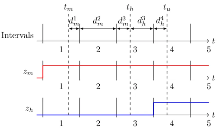
Durations dm(j, i) and dh(j, i) depend on operation start times tm(j), th(j)
and tu(j), and the intervals to which they belong. Binary variables are used to
identify the intervals in which energy (for melting or holding) is supplied to the furnace for job j. Variables zm(j, i) indicate if melting start time of job j occurred
before or during interval i. Similarly, zh(j, i) and zu(j, i) indicate if holding and
unloading start times of job j occurred before interval i. For example, Figure 3 shows zm(j, i) and zh(j, i) for the same job as in Figure 2. The melting operation
Furnace
t
load. heating unload.
tm th tu Melting Holding Power t e1 m e2 m e3 m 1 2 3 4 5 Pmin Pmax Phold Intervals t 1 2 3 4 5 d1 m d2m d3m d 3 h d 4 h
Figure 2 Energy supply by interval: melting and holding.
Intervals t 1 2 3 4 5 d1 m d2m d3m d 3 h d 4 h zm t 1 2 3 4 5 zh t 1 2 3 4 5 tm th tu
Figure 3 Time/interval binary variables.
The following equations give the relations between the melting start time and binary variable zmfor all job j in J , according to the above description. Constraints
for zhand zu are similar.
tm(j) ≥ D.i(1 − zm(j, i)) i = 1, . . . , Imax− 1 (11)
tm(j) ≤ D.i + M (1 − zm(j, i)) i = 1, . . . , Imax− 1 (12)
zm(j, i + 1) ≥ zm(j, i) i = 1, . . . , Imax− 1 (13)
zm(j, Imax) = 1 (14)
The sequence of operations and the sequence of jobs induce additional con-straints between time/interval variables. Equations (15) and (16) are based on the
melting-holding-unloading sequence; (17) is related to precedence constraints. zm(j, i) ≥ zh(j, i + 1) ∀j ∈ J, i ∈ [1..Imax− 1] (15)
zh(j, i) ≥ zu(j, i) ∀j ∈ J, i ∈ I (16)
zu(j1, i) ≥ zm(j2, i) − (1 − y(j1, j2))
∀(j1, j2) ∈ J2, i ∈ I (17)
3.2.2 Melting duration and energy.
The melting operation of a job, between tmand th, is decomposed in intervals
(Fig. 2). Melting duration dm(j, i) of any interval i lies in [0, D]. It is zero if
zh(j, i) − zm(j, i) = 0 (Fig. 3, (18)). The sum of all interval durations is equal to
the overall melting duration (19).
0 ≤ dm(j, i) ≤ D(zm(j, i) − zh(j, i)) ∀j ∈ J, i ∈ I (18)
X
i∈I
dm(j, i) = th(j) − tm(j) ∀j ∈ J (19)
Note that when tm(j) exactly matches the end of an interval i (tm(j) = D.i),
zm(j, i) can either take the value 0 or 1 ((11) and (12)). This is not a problem
because in this case dm(j, i) = 0 whatever the value of zm(j, i) (19).
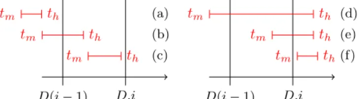
The duration of melting dm(j, i) for an interval i depends on the position of the
melting and holding start times with respect to this interval. Figure 4 summarizes the possible configurations of tmand thover an interval i. The corresponding value
of dmis the intersection of interval i and [tm, th].
D(i − 1) D.i tm th (a) tm th (b) tm th (c) D(i − 1) D.i tm th (d) tm th (e) tm th(f)
Figure 4 Intersections of a melting operation and an interval.
The following constraints set the value of dm(j, i) according to these
configura-tions, for all i in {2, . . . , Imax− 1} and j in J :
dm(j, i) ≥D(zm(j, i − 1) − zh(j, i + 1)) (20)
dm(j, i) ≥D.i(1 − zm(j, i − 1)) − tm(j)
− D.zh(j, i + 1) (21)
dm(j, i) ≥th(j) − D.i + D.zm(j, i − 1)
− M (1 − zh(j, i + 1)) (22)
Constraints (20), (21) and (22) respectively match configurations (d), (e) and (b). The other cases are solved by (18) and (19).
For each interval, the amount of energy provided to a job depends on the melting duration and the supplied power. The melting ends when the required energy quantity E(j) is reached.
Pmin.dm(j, i) ≤ em(j, i) ≤ Pmax.dm(j, i) ∀j ∈ J, i ∈ I (23)
X
i∈I
em(j, i) = E(j) ∀j ∈ J (24)
3.3 Operator unavailability
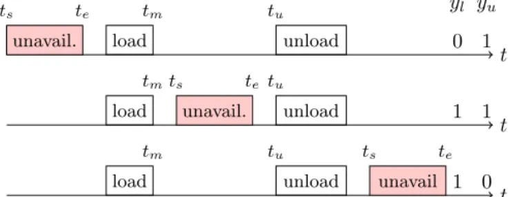
Unavailability may occur when the number of furnaces exceeds the number of operators. In this case, at the end of the melting operation the material stays in the furnace and the temperature is hold, involving extra energy consumption at power Phold, until an operator become available to unload the furnace. These human
resource constraints are represented by unavailabilities, modelled as operations on a furnace. Operator unavailability o is defined by its start time ts(o), end time
te(o) and the binary parameter Xo(o, f ) = 1 if unavailability o is on furnace f , 0
otherwise. An unavailability cannot overlap a loading or unloading operation on the same furnace, but can overlap a melting operation. Consequently, according to the position of loading and unloading, three configurations of a job j and an unavailability o are possible (Fig. 5).
yl yu ts te tm tu t load unload unavail. 0 1 t ts te tm tu
load unavail. unload 1 1
t
ts te
tm tu
load unload unavail 1 0
Figure 5 Relative positions job/unavailability.
Binary variables yl(j, o) and yu(j, o) represent the relative position of
load-ing/unloading and unavailability (Fig. 5). At least one is equal to 1 if the un-availability and the job are on the same furnace:
yl(j, o) + yu(j, o) ≥ Xo(o, f ) + x(f, j) − 1 (25)
The following set of constraints links operations start times with unavailability start and end times, for all j in J and o in O:
tm(j) ≤ ts(o) + M (1 − yl(j, o)) (26)
tm(j) − Dl(j) ≥ te(o) − M (1 + yl(j, o) − yu(j, o)) (27)
tu(j) + Du(j) ≤ ts(o) + M (1 − yl(j, o) + yu(j, o)) (28)
tu(j) ≥ te(o) − M (1 − yu(j, o)) (29)
Constraints (26) to (29) give the relative position of tm(j), tu(j), ts(j) and te(j)
for the cases yl= 1, yl= 0 and yu= 1, yu= 0 and yl= 1, and yu= 1 respectively
3.4 Objective function
If there is no operator available to unload the furnace, holding is carried out with a power Phold during dh. Thus the overall energy for an interval is the sum of
melting and holding energy on each furnace. se(i) =X
j∈J
(em(j, i) + Phold.dh(i, j)) ∀i ∈ I (30)
Value se(i) is then used to evaluate the instantaneous power, as the mean power over interval i. Power overrun ov(i) is noticed on an interval when this power exceeds the subscribed power Ps.
ov(i) ≥ se(i)/D − Ps ∀i ∈ I (31)
ov(i) ≥ 0 ∀i ∈ I (32)
The objective function (33) minimizes the cost of the energy consumption and the overrun cost:
minX
i∈I
(α.se(i) + β.ov(i)) (33)
Finally, given the hypothesis thatP
i∈Iem(j, i) = Ej whatever the melting profile,
the objective function can be written as the sum of the holding energy cost and the overrun cost: minX i∈I (α.Phold. X j∈J dh(i, j) + β.ov(i)) (34) 3.5 Problem complexity
The problem under consideration in this paper is strongly NP-hard. This can be shown by considering a special case where the number of machines is larger than the number of jobs, there are no machine unavailability, there are zero loading and unloading times, D = 1 and Pmin = Pmax. In this case answering the question
whether no overrun is observed is NP-complete in the strong sense as we obtain the multiprocessor task problem P |ri, di; sizei|− (Drozdowski, 1996).
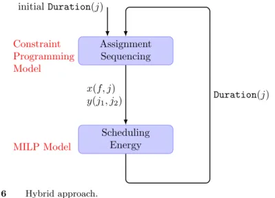
4 A heuristic hybrid method
The integer linear program proposed in the preceding section is only able to solve small problems. To deal with real-life problems, we propose a two-step heuristic method based on the decomposition of the problem into two decision steps (Fig. 6). During the first step, sequencing of jobs on the furnaces is performed with fixed job durations. Since it may happen that no feasible solution exists considering the due dates, due date violation is admitted but the objective is to minimize the maximal tardiness. Hence the problem resorts to a parallel machine problem which machine availability, release dates and maximal tardiness criterion. A particularity
of the problem is that unavailability concerns only the loading and unloading parts of the jobs.
During the second step, the job sequence is fixed on the furnaces according to the preceding step and the jobs are precisely scheduled while the power setting of each furnace during each interval determines the precise duration of each job. The objective function is the same as in Section 3.4 with an additional term to highly penalize due date violations.
For the first iteration, step 1 is performed by considering fixed melting durations of the jobs corresponding to the maximal power Pmax given to the furnace. Then
we close the loop by using at step 1 the durations given by step 2. The process is interrupted if the objective function of step 2 is not better than the one of the previous iteration, and if the tardiness is not improved.
Constraint Programming Model Assignment Sequencing MILP Model Scheduling Energy x(f, j) y(j1, j2) Duration(j) initial Duration(j)
Figure 6 Hybrid approach.
Step 1 of the proposed heuristic corresponds to solving an almost standard par-allel machine scheduling problem. Any specialized algorithm can be adapted to solve this problem. We propose a constraint programming approach to tackle this problem. Step 2 of the proposed method involves continuous start times and power intensity variables. Linear programming is a particularly well-suited technique to tackle the problem. In Section 4.1, we present the constraint programming frame-work. In Section 4.2, we present the link with the integer linear programming part.
4.1 Modeling and solving the furnace assignment and job sequencing problem We propose to use a commercial constraint programming modeling language and solver (IBM ILOG OPL 6.3/CP Optimizer 2.3) to cope with the parallel machine problem corresponding to step 1. The OPL language provides high level primitives to model scheduling components. We provide the OPL code in Figures 7, 8 and 9. As a first category of high level scheduling components, task declaration is displayed in Figure 7. Job loading, melting and unloading, and furnace unavailabilities are
// Tasks
dvar interval loading [j in J] in ReleaseDate[j]..maxint size LoadDuration[j]; dvar interval melting [j in J]
in ReleaseDate[j]+LoadDuration[j]..maxint size Duration[j] ;
dvar interval unloading [j in J]
in ReleaseDate[j]+LoadDuration[j]+Duration[j]..maxint size UnloadDuration[j];
dvar interval unavail [o in O]
in unavailEarliestStart[o]..unavailLatestEnd[o] size UnavailDuration[o];
// Optional tasks: possible assignements of a furnace to a task dvar interval alt_loading [f in F] [j in J]
optional in ReleaseDate[j]..maxint size LoadDuration[j];
dvar interval alt_melting [f in F] [j in J] optional in ReleaseDate[j]+LoadDuration[j]..maxint size Duration[j] ;
dvar interval alt_unloading [f in F] [j in J]
optional in ReleaseDate[j]+LoadDuration[j]+Duration[j]..maxint size UnloadDuration[j];
Figure 7 Constraint programming: task declarations.
// Sequence of jobs on furnace f dvar sequence jobSequence[f in F] in
append(all(j in J) alt_loading[f][j], all(j in J) alt_melting[f][j], all(j in J) alt_unloading[f][j]);
// Sequence of tasks requiring an operator on furnace f dvar sequence unavailSequence[f in F] in
append(all(j in J) alt_loading[f][j], all(j in J) alt_unloading[f][j],
all(o in O: UnavailFurnace[o]==f)unavail[o]);
Figure 8 Constraint programming: sequence declarations.
defined as tasks (type dvar interval) specifying for each of them the time windows (field in) and the duration (field size). Furthermore optional tasks are associated to each loading, melting and unloading tasks to model the furnace assignment problem, so that there exists an optional task per loading, melting and unloading operation and candidate furnace. As indicated above, Duration[j] for the melting part of job j is initially set to minimal value E(j)/Pmax.
In Figure 8, two sets of sequences (type dvar sequence) are declared as a second high level scheduling component category. The first set comprises a sequence declared per furnace f , gathering each optional loading, melting and unloading task assigned to f . The second set also contains a sequence of tasks per furnace f , gathering the optional loading and unloading operations assigned to f and the unavailability tasks assigned to f . It is used to manage the operator availability constraints.
Figure 9 now describes the constraints on the scheduling components and the objective function. First the objective is maximal tardiness minimization as the due dates are relaxed. Then, for each job the loading, melting and unloading tasks are constrained to be synchronized: melting operation of a job starts at the end of loading and unloading starts at the end of melting. The next two sets of constraints
minimize max(j in J) maxl(0,endOf(unloading[j])-DueDate[j]); subject to{
// Job tasks synchronization forall(j in J) { startAtEnd(melting[j],loading[t],0); startAtEnd(unloading[t],melting[t],0); } // Furnace assignment forall(j in J) {
alternative(loading[j], all(f in F) alt_loading[f][j]); alternative(melting[j], all(f in F) alt_melting[f][j]); alternative(unload[j], all(f in F) alt_unloading[f][j]); }
// All the tasks of a job on the same furnace forall(j in J,f in F) {
presenceOf(alt_loading[f][j])==presenceOf(alt_melting[f][j]); presenceOf(alt_melting[f][j])==presenceOf(alt_unloading[f][j]); }
// Furnaces viewed as disjunctive resources forall(f in F) {
noOverlap(jobSequence[f]); noOverlap(unavailSequence[f]); }
}
Figure 9 Constraint programming: objective and constraints.
are about assignment: we define each loading, melting and unloading task as an alternative among all corresponding optional tasks. It follows that for a given loading, melting or unloading task, only one optional task will be activated. Then we state that the optional loading, melting and unloading tasks of a same job must be assigned to the same furnace. The last set of constraints describes how the two sets of sequences are handled. In this case, no overlapping of the tasks belonging to each sequence is allowed.
Once written in OPL, the parallel machine problem can be solved by the IBM ILOG CP Optimizer, a commercial constraint programming solver embedding prece-dence and resource constraint propagation techniques and an efficient self-adapting large neighborhood search method dedicated to scheduling problems (Laborie, 2009). A time limit is set and the best solution found within the time limit is returned. Note that modeling unavailabilities as tasks allows to define a time window for positioning each unavailability period.
4.2 Solving the scheduling and power setting problem with fixed furnace assignment and job sequences
In the second stage of the proposed heuristic, the MILP model presented in Section 3 (equations (4) to (34)) is used to set precise job start times and power supply while keeping the job assignments and sequences found at the previous stage. Due dates can be violated but tardiness is highly penalized in order to seek for a feasible final solution. Hence the heuristic does not stop if, for a given iteration, the MILP problem has no solution that respects the due dates. A time limit is set and the best solution found within the time limit is returned. If this solution has no tardiness, no overrun and no holding, the loop is broken because the optimum is reached.
4.3 Variant: initial melting durations for Step 1
The OPL modeling language gives the opportunity to define a job duration as a range between two values. Thus the melting interval variables can be defined as a range [Ej/Pmax; maxint], letting the solver determine the adequate duration
between the minimal duration and a value that represents the sum of maximal and holding durations. Using this feature at the first iteration may limit the number of iterations if task durations well reflect energy consumption. To this aim, a term is added to tardiness in the objective function of Step 1, that penalizes tasks whose duration is far from the maximal duration. Indeed, when duration is close to the minimum value, the furnace is set to a high power and it could lead to power overrun. On the other hand, if the duration is higher than the maximal duration, holding energy is spent. For the next iterations, the original hybrid approach is used, with the previous CP model at Step 1 relying on the durations given by Step 2.
5 Experimental results
Experimental results give an idea of the interest of the two-level heuristic. The following results are based on the pipe-manufacturing example: we consider 9-hour working days (from 8 am to 5 pm) with operator unavailability during lunch break (from 12:00 am to 1:30 pm) and during the morning and afternoon breaks (15’ between 10:00 and 10:30 am, and 15’ between 3:00 and 3:30 pm). The flexibility of morning and afternoon breaks allowed to reduce power overrun, inducing a signifi-cant cost reduction (Ha¨ıt et al., 2007). Instances of 36 jobs on 6 furnaces are tested. Job energy requirements and release and due dates were randomly generated. En-ergy consumption is calculated on 15’ periods. EnEn-ergy cost is $0,0242 /kWh, and the penalty for overrun is $32 for each kW over the subscribed power.
All the tests have been performed on a SUN Sunfire server with four Quad-Core AMD Opteron(tm) 2.5 GHz Processors. Parallel CPLEX 12.1 is used to solve the MILP problems. Time limits are set for the hybrid approach thus bounding an iteration duration: 30 s for Step 1 (CP) and 180 s for Step 2 (MILP).
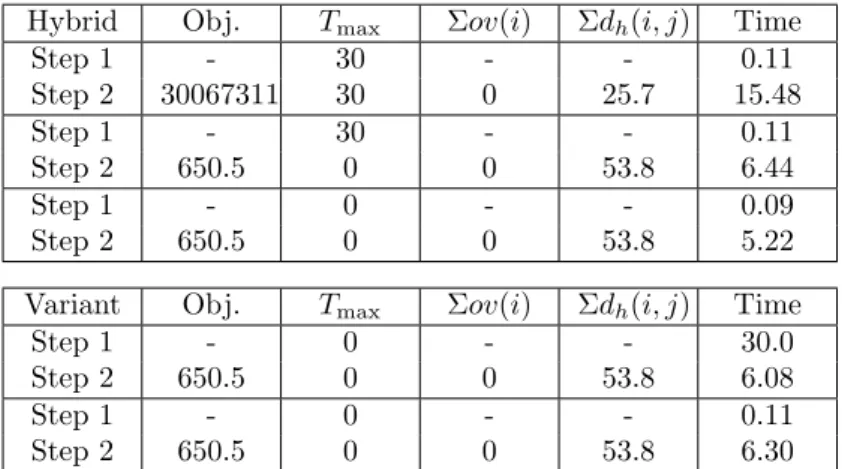
5.1 Solution steps on an illustrative instance
Table 1 shows the solution steps for an illustrative problem instance (data given in appendix B), with MILP model, hybrid model with fixed initial durations and variant hybrid model with variable initial durations. The tables give the objective value, the maximal tardiness, the sum of power overruns and of holding durations, and the computation time.
Table 1 Illustrative instance solved with MILP and Hybrid approaches
Obj. Tmax Σov(i) Σdh(i, j) Time
Hybrid Obj. Tmax Σov(i) Σdh(i, j) Time Step 1 - 30 - - 0.11 Step 2 30067311 30 0 25.7 15.48 Step 1 - 30 - - 0.11 Step 2 650.5 0 0 53.8 6.44 Step 1 - 0 - - 0.09 Step 2 650.5 0 0 53.8 5.22
Variant Obj. Tmax Σov(i) Σdh(i, j) Time
Step 1 - 0 - - 30.0
Step 2 650.5 0 0 53.8 6.08
Step 1 - 0 - - 0.11
Step 2 650.5 0 0 53.8 6.30
The MILP model is solved to optimality in more than 20 minutes. Compared to this solving time, the hybrid approach is very fast. At the first step, the method gives a solution with tardiness, due to the initial values. The assignment and sequencing variables are sent to Step 2, and a first solution is given. The result is big because of the huge penalty given to tardiness. At the second iteration, a solution with tardiness is found again by the CP solver at Step 1, but Step 2 gives then a solution with only a holding duration greater than 0. Note that it is the optimal solution. A third iteration is performed. As nothing is improved, the process ends. The overall solving duration is less than 30 seconds, and no iteration time limit has been reach.
Although the minimal durations are taken to initialize the process for the hybrid approach, the first step of the first iteration does not give a solution with no tardi-ness (it is only found at iteration 3). This is due to unavailability periods. Fixed melting durations do not necessary fit with these periods so that loading would be performed before an unavailability period and unloading after it. The variant approach attempts to solve this problem by improving the solution quality at the first step or the first iteration. The results are given in the last part of Table 1. The solution with no tardiness is found at the first iteration. Only two iterations are necessary to find the best solution. However, the first step of the first iteration lasts 30 seconds (the search is interrupted by the time limit), and the total duration is higher than the hybrid approach duration. Hence the variant should be interesting if the MILP solving time become longer and if the quality of the final solution is closely linked to the quality of the first iteration solution.
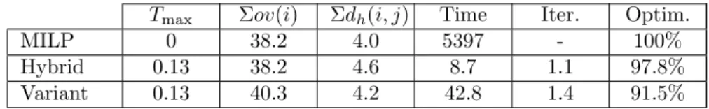
5.2 Method comparison on randomly generated problem instances
A set of 100 problem instancesa with 36 jobs and 6 furnaces were generated according to the parameters described above, inspired by the industrial case study. Among these, 47 were found feasible by the MILP solver and solved to optimality while the others were proven unfeasible. In this section, we compare the MILP, hybrid and variant models on these instances.
Table 2 summarizes the results of MILP, hybrid and variant approaches for the 47 feasible instances. MILP solving time stays high so that using this model would
be difficult in a situation with hundred of jobs. Some instance have overrun or holding durations in their optimal solution.
Table 2 Comparison of the approaches: mean values on 47 feasible instances
Tmax Σov(i) Σdh(i, j) Time Iter. Optim.
MILP 0 38.2 4.0 5397 - 100%
Hybrid 0.13 38.2 4.6 8.7 1.1 97.8%
Variant 0.13 40.3 4.2 42.8 1.4 91.5%
The hybrid approach is very fast, with a mean solving time less than 10 seconds. Only one instance has not been solved to optimality. Most of the instances have been solved in one iteration. Compared to this excellent result, the variant is less interesting: four instances have not been solved to optimality and the solving time is higher. Note that for some instances, tardiness is greater than 0, so the solution found is not feasible.
5.3 Comparison on bigger instances
In this section we present how processing time increases with the size of the instances. MILP solving time grows extremely rapidly with the number of jobs, furnaces and intervals, so we do not compare these results with optimal solutions. The results are based on the same one-day shift instances with operator unavail-abilities, inspired from the industrial case. Mean values on 50 randomly-generated instances are given.
At first we present in Table 3 the results of hybrid approach for the same problem as previously, but with smaller intervals so that the number of intervals increases as the horizon remains the same. The increase of intervals affects Step 2 (MILP model). Objective values cannot be compared because power overrun are not calcu-lated on the same basis (interval durations). Solving time grows with the number of intervals. This is mainly due to MILP solving at Step 2. In the case of 90 intervals, time limit has been change in order to give the solver enough time to find solutions.
Table 3 Hybrid approach with growing number of intervals
36 54 72 90
Time 18.6 96.9 336.7 983.1
Iterations 1.94 1.90 2.18 2.81
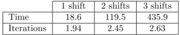
Then we propose to solve globally two or three consecutive shifts, so the num-ber of tasks will be respectively 72 and 108 instead of 36. The numnum-ber of furnaces does not change. Table 4 presents the mean solving time and iteration number for 50 instances (feasible or not). The number of iterations does not increase rapidly, whereas the solving time does. Again, this is mainly due to MILP solving. For the 3-shift instances, the 180-second time limit is often reached at Step 2.
When the size of the problem increases, the MILP solving at Step 2 of the hybrid approach may take some time, even if it is much better than the full MILP solving.
Table 4 Hybrid approach with growing number of tasks
1 shift 2 shifts 3 shifts
Time 18.6 119.5 435.9
Iterations 1.94 2.45 2.63
This is due to symmetries in the model. The solution is given in a reduced number of iterations, because the loop is broken as soon as the solution is not improved. Consequently, the increase of the problem size may affect the quality of the solution if the MILP solver does not have enough time to give a good solution. The first action would be to increase the MILP time limit, as done in Table 3 for 90-interval instances. This also claims for an improved variant approach in order to find a better initial solution. CP models that account for energy should be more adapted to the problem (Artigues et al., 2009).
6 Conclusion-Future work
In this paper we presented a mathematical/constraint programming heuristic approach to solve a foundry scheduling problem with energy and human resource constraints. The implemented methods are based on an iterative succession of a sequencing and assignment on parallel machines of jobs with fixed or variable durations via CP and a power adjustment and precise scheduling phase via MILP. The results are satisfactory since the proposed hybrid methods reach near-optimal solutions in reasonable CPU times on the computational experiments we carried-out using realistic data. In particular, the CPU times are drastically reduced compared to the full MILP model. Additional tests will be performed on other instances and other problem variants, like configurations with a number of operators lower than the number of furnaces. Future work will also focus on improving the method. The improvement of the first step may help to get good solutions rapidly. To this aim, this step could take into account explicitly energy constraints.
References
M. Agha, R. Thery, G. Hetreux, A. Ha¨ıt, and J.-M. Le Lann. Integrated production and utility system approach for optimizing industrial unit operations. Energy, 35(2):611–627, 2010.
M. Agha, R. Thery, G. Hetreux, and J.-M. Le Lann. Mod`ele int´egr´e pour l’ordonnancement d’ateliers batch et la planification de centrales de cog´en´ era-tion. Conf´erence Internationale de Mod´elisation et Simulation, MOSIM08, Paris, France, 2008.
C. Artigues, P. Lopez, and A. Ha¨ıt. Scheduling under enregy constraints. Pro-ceedings of the International Conference on Industrial Engineering and Systems Management (IESM’09), 2009.
Ph. Baptiste, A. Jouglet, C. Le Pape, and W. Nuijten. A constraint-based approach to minimize the weighted number of late jobs on parallel machines, 2000. UTC Technical Report 2000/288.
E.-K. Boukas, A. Haurie, and F. Soumis. Hierarchical approach to steel production scheduling under a global energy constraint. Annals of Operations Research, 26:289–311, 1990.
Z.-L. Chen and W. B. Powell. Solving parallel machine scheduling problems by column generation. INFORMS J. on Computing, 11(1):78–94, 1999.
T. Cheng and C. Sin. A state-of-the-art review of parallel-machine scheduling research. European Journal of Operational Research, 47:271–292, 1990.
K.-Y. Cheung and C.-W. Hui. Total-site scheduling for better energy utilization. Journal of Cleaner Production, 12:171–184, 2004.
Maciej Drozdowski. Scheduling multiprocessor tasks – an overview. European Jour-nal of OperatioJour-nal Research, 94:215–230, 2004.
B. Gacias, C. artigues and P. Lopez. Parallel machine scheduling with prece-dence constraints and setup times. Computers and Operations Research, doi:10.1016/j.cor.2010.03.003, 2010.
D. Gibbs and P. Deutz. Reflexion on implementing industrial ecology through eco-industrial park development. Journal of Cleaner Production, 15(17):1683–1695, 2007.
A. Ha¨ıt, C. Artigues, M. Trepanier, and P. Baptiste. Ordonnancement sous con-traintes d’´energie et de ressources humaines. 11e congr`es de la Soci´et´e Fran¸caise de G´enie des Proc´ed´es, Saint-Etienne, France, R´ecents progr`es en G´enie des Proc´ed´es, 96, 2007.
I. Harjunkoski and I. Grossmann. A decomopsition approach for the scheduling of a steel plant production Computers and Chemical engineering, 25:1647–1660, 2001.
S. Irani and K. Pruhs. Algorithmic problems in power management. SIGACT News, 36(2):63–76, 2005.
J. Korhonen. A material and energy flow for co-production of heat and power. Journal of Cleaner Production, 10:537–544, 2002.
P. Laborie. IBM ILOG CP optimizer for detailed scheduling illustrated on three problems. Proceedings of the 6th International Conference, on Integration of AI and OR Techniques in Con- straint Programming for Combinatorial Optimization Problems (CP-AI-OR’09), LNCS 5547: 148–162, 2009.
E. N´eron, F. Tercinet, and F. Sourd. Search tree based approches for parallel machine scheduling. Computers and Operations Research, 35(4):1127–1137, 2008. K. Nolde and M Morari. Electrical load tracking scheduling of a steel plant
W. L. Pearn, S. H. Chung, and C .M. Lai. Scheduling integrated circuit assembly operations on die bonder. IEEE Transactions on electronics packaging manufac-turing, 30(2), 2007.
Ruslan Sadykov and Laurence A. Wolsey. Integer programming and constraint pro-gramming in solving a multimachine assignment scheduling problem with dead-lines and release dates. INFORMS Journal on Computing, 18(2):209–217, 2006. A. Salem, G. C. Anagnostopoulos, and G. Rabadi. A branch-and-bound algorithm for parallel machine scheduling problems. In Harbour, Maritime & Multimodal Logistics Modeling and Simulation Workshop, Society for Computer Simulation International (SCS), Portofino (Italy), 2000.
A Notation A.1 Parameters
Indices
j Job (J set of jobs)
f Furnace (F set of furnaces)
o Unavailability (O set of unavailabilities) i Interval (I set of intervals)
Power parameters
Pmin Minimal furnace power
Pmax Maximal furnace power
Phold Holding power
Ps Subscribed power
Job parameters
Dl(j) Loading duration of job j
Du(j) Unloading duration of job j
E(j) Energy required for job j Rel(j) Release date of job j Due(j) Due date of job j Interval parameters
Imax Number of intervals
D Duration of an interval Unavailability parameters
A.2 Continuous variables Energy-related variables
em(j, i) Melting energy for job j during interval i
dm(j, i) Melting duration for job j during interval i
dh(j, i) Holding duration for job j during interval i
se(i) Total energy consumption during interval i ov(i) Power overrun during interval i
Operation-related variables
tl(j) Loading start time of job j
tm(j) Melting start time of job j
th(j) Holding start time of job j
tu(j) Unloading start time of job j
ts(o) Unavailability o start time
te(o) Unavailability o end time
A.3 Binary variables Allocation variables
x(f, j) Allocation of furnace f to job j Precedence variables
y(j1, j2) Precedence between jobs j1 and j2
yl(j, o) Precedence between loading operation
of job j and unavailability o
yu(j, o) Precedence between unloading operation
of job j and unavailability o Relative time/interval position variables
zm(j, i) Melting start time tm(j) w.r.t. interval i
zh(j, i) Holding start time th(j) w.r.t. interval i
zu(j, i) Unloading start time tu(j) w.r.t. interval i
B Instance data NbJobs=36; NbFurnaces=6; NbUnavail=18; Imax=36; D=25; Pmin=500; Pmax=1200; Phold=500; Ps=3000; F1=0.0242; F2=32; Dl=[22 14 24 23 19 11 23 18 9 12 23 2 11 7 0 0 4 15 11 0 10 3 7 1 23 15 0 9 13 20 0 7 24 23 12 10 ]; Du=[23 13 22 25 5 8 21 17 23 16 22 13 3 20 8 14 18 25 10 17 10 14 4 24 22 5 20 14 23 4 16 18 18 24 17 20 ]; E=[74831 50285 62357 61938 36862 32296 58587 31681 52931
18904 55966 39281 23118 40268 69629 31891 43927 21161 48091 67305 35053 63856 72285 61409 25944 45552 23373 60472 49108 57937 43054 48575 21695 38225 44270 72462 ]; Rel=[83 395 695 299 222 315 530 112 141 575 409 835 370 84 792 334 182 780 4 537 90 75 453 349 364 689 715 483 318 42 75 802 517 194 102 441 ]; Due=[755 576 859 500 571 787 749 277 263 850 825 896 503 280 895 743 514 876 793 683 665 548 612 812 581 772 871 737 748 145 266 885 723 886 736 738 ]; Xo=[ [1 0 0 0 0 0 ] [1 0 0 0 0 0 ] [1 0 0 0 0 0 ] [0 1 0 0 0 0 ] [0 1 0 0 0 0 ] [0 1 0 0 0 0 ] [0 0 1 0 0 0 ] [0 0 1 0 0 0 ] [0 0 1 0 0 0 ] [0 0 0 1 0 0 ] [0 0 0 1 0 0 ] [0 0 0 1 0 0 ] [0 0 0 0 1 0 ] [0 0 0 0 1 0 ] [0 0 0 0 1 0 ] [0 0 0 0 0 1 ] [0 0 0 0 0 1 ] [0 0 0 0 0 1 ] ]; So=[400 150 650 400 150 650 400 150 650 400 150 650 400 150 650 400 150 650 ]; Eo=[500 250 750 500 250 750 500 250 750 500 250 750 500 250 750 500 250 750 ]; Do=[100 25 25 100 25 25 100 25 25 100 25 25 100 25 25 100 25 25 ];