FINITE ELEMENT APPROXIMATION OF AN OPTIMAL DESIGN PROBLEM

(1)

HAL Id: hal-00678439

https://hal.archives-ouvertes.fr/hal-00678439

Submitted on 12 Mar 2012

HAL is a multi-disciplinary open access archive for the deposit and dissemination of sci-entific research documents, whether they are pub-lished or not. The documents may come from teaching and research institutions in France or abroad, or from public or private research centers.

L’archive ouverte pluridisciplinaire HAL, est destinée au dépôt et à la diffusion de documents scientifiques de niveau recherche, publiés ou non, émanant des établissements d’enseignement et de recherche français ou étrangers, des laboratoires publics ou privés.

FINITE ELEMENT APPROXIMATION OF AN

OPTIMAL DESIGN PROBLEM

Abdelkrim Chakib, Abdeljalil Nachaoui, Mourad Nachaoui

To cite this version:

Abdelkrim Chakib, Abdeljalil Nachaoui, Mourad Nachaoui. FINITE ELEMENT APPROXIMATION OF AN OPTIMAL DESIGN PROBLEM. Journal of Applied and Computational Mathematics, 2012, 11 (1), pp.19-26. �hal-00678439�

(2)

FINITE ELEMENT APPROXIMATION OF AN OPTIMAL DESIGN PROBLEM

A. CHAKIB1_{, A. NACHAOUI}2_{, M. NACHAOUI}1,2

Abstract. This paper investigates shape optimization of complex thermo-fluid phenomena

that occur in welding processes. The linear finite elements dicretization is accomplished. The existence of the discrete optimal solution is established. Some computational results for our approach are presented and discussed.

Keywords: Shape Optimization, Free Boundary, Non Coercive Operator, Welding, Finite Ele-ment, Genetic Algorithms.

AMS Subject Classification: 49Q10, 35R35, 65N30.

1. Introduction

In this paper, we consider a problem modeling analysis of heat transfer in a welding operation. The aim is to identify the liquid/solid interface and estimate the field temperature in the welded parts of the plate in order to predict and control the mechanical effects caused by the process on these parts (residual stresses, distortions. . . ). The considered approach concerned only the solid part of the plate and it consists to simplify the physical phenomena occurring between the welding torch and the plate as well as the liquid bath by introducing a temperature condition imposed on the liquid/solid interface which is unknown. To solve this free boundary problem, an optimal shape design formulation was proposed in [4]. Our interest is the numerical study of the approached shape design problem, obtained by using the finite element method and the parametrization of the liquid/solid interface by B´ezier curves. We are interested more precisely by showing the existence of the optimal discrete solution of this approached problem. The main difficulty of this work lies in the fact that the state problem is governed by a noncoercive operator, which complicates the study of existence. At this stage, it must be noted that in the coercive case we can show easily this result, see [8]. The proposed approach for overcoming this difficulty is based on the topological degree tools in finite dimensional spaces [6], and a uniform estimate of discrete solutions norm’s. To show the efficiency of our approach, we give some numerical results.

2. Setting of the problem

We are interest by a numerical realization, using the finite element method, of the optimal shape design formulation of a welding problem given by

1_{Laboratoire de Mathématiques et Applications Université Sultan Moulay slimane, Faculté des Sciences et}

Techniques, B.P.523, B´eni-Mellal, Maroc, e-mail: mourad.nachaoui@univ-nantes.fr

2_{Laboratoire de Mathématiques Jean Leray UMR6629 CNRS Université de Nantes 2 rue de la Houssinière,}

BP92208 44322 Nantes, France, e-mail: mourad.nachaoui@univ-nantes.fr Manuscript received 29 April 2011.

(3)

2 APPL. COMPUT. MATH., V.11, N.1, 2012                      find Ω∗_{∈ Θ} ad solution of J(Ω∗) = inf Ω∈Θad J(Ω) where J(Ω) = 1₂R_Γ₀|T (Ω(x, y)) − T0|2dσ

and T (Ω) the solution of

(SP )    K∂T_∂x = ∇ · (λ∇T ) + f in Ω λ∂T_∂ν = 0 on Γ0∪ Γ1∪ Γ2∪ Γ3 T = Td on Γ4, T = Tf on Γ, (1)

where the parameters in (1) are such that:

K is a constant dependent to the material characteristics (density of the plate and heat capac-ity,...), λ is the thermal conductivity, f is a given source term. The quantities Td, T0 and Tf are

given temperatures. The solid part of plate Ω (see fig. 1), is defined by

Figure 1. The solid part of the welded workpiece with interface Γ.

Ω(ϕ) =]0, a[×]0, Ly[∪

©

(x, y) ∈ IR2/a ≤ x ≤ b, ϕ(x) ≤ y ≤ Ly

ª

∪]b, Lx[×]0, Ly[ (2)

where ϕ, the parametrisation of the unknowon boundary Γ, is a Lipschitz function. The set Θad

is defined by

Θad= {Ω(ϕ) ϕ ∈ Uad}

and Uad =

©

ϕ ∈ C([a, b]) / ∃ aϕ and bϕ∈ [a, b] , ϕ|[a,aϕ]= 0 , ϕ|[bϕ,b] = 0 and ∃ L0> 0 /

¯ ¯ϕ(x) − ϕ(x′₎¯_{¯ ≤ L} 0 ¯ ¯x − x′¯_{¯ ∀x, x}′ _{∈ [a, b] , 0 ≤ ϕ(x) ≤ L} y ∀x ∈ [a, b] ª .

In the sequel we suppose that the parameters of our problem are such that: D =]0, Lx[×]0, Ly[,

(H1) λ ∈ L∞(D) and ∃λ0 > 0 such that λ(x)ξ · ξ ≥ λ0|ξ|2 a.e x ∈ D

(H2) K ∈ L∞(D) and f ∈ L2(D)

Let ΓD = Γ ∪ Γ4, we define the space HΓ1D(Ω) =

©

u ∈ H1(Ω) / u|ΓD = 0

ª

where H1(Ω) is the Sobolev space. From the surjectivity of the trace operator from H1_{(D) to H}1₂_{(∂D), we have}

∃ V ∈ H1(D) such that V = ½

v on ]b, Lx[×]0, Ly[

Tf on ]0, b[×]0, Ly[,

where v ∈ H1(]b, Lx[×]0, Ly[) such that v = Td on Γ4 and v = Tf on {b} × [0, Ly] .

Then a variational formulation of the state problem (SP ) is the following: ½ find u ∈ H_Γ1_D(Ω) R Ωλ∇u · ∇ψ + R ΩK ψ∂u∂x = R Ωf ψ − R Ωλ∇V · ∇ψ − R ΩK ψ∂V∂x ∀ψ ∈ HΓ1D(Ω). (3)

(4)

Theorem 1. Under assumptions (H1) and (H2), the problem (1) is well posed and admits

at least one solution in Θad.

3. Numerical approximation of the problem

In this section we give an approximation of (1); we shall discretize both the admissible family Θad and the state problem (SP). We start with the first one, for this we use the piecewise spline

approximations of Γ(ϕ) locally realized by quadratic B´ezier functions [8].

3.1. Discretization of the shape optimal problem. Let us consider a uniform partition (ai)di=0 of [a, b], such that a = a0 < a1 < ... < ad = b, ai = iµ + a, µ = (b − a)/d, i = 0, ..., d;

and a_i+1/2 be the midpoint of [ai, ai+1]. Further let Ai = (ai, ϕi), ϕi ∈ IR, i = 0, ..., d, be design

nodes and A_i+1/2 = 1₂(Ai+Ai+1) be midpoint of the segment AiAi+1, i = 0, ..., d−1. In addition

let a₋1 2 = a − µ 2, ad+1₂ = b + µ 2, A−1₂ = (a−1₂,12(ϕ0+ ϕ1)), Ad+1₂ = (ad+1₂,12(ϕd−1+ ϕd)).

Remark 1. The triple {A_i−1

2, Ai, Ai+ 1

2}, is termed the control points of the B´ezier function.

For a partition (ai)di=0we associate the set Qadµ ⊂ Uadof continuous, piecewise linear functions

over (ai)di=0:

Qad_µ = {ϕµ∈ C([a, b]) | ϕµ|[ai−1,ai]∈ P1([ai−1, ai]) ∀i = 1, ..., d} ∩ Uad. (4)

The family of admissible discretized design domains is now represented by

Θµ_ad = { Ω(sµ) /sµ∈ U_adµ, } (5) where U_adµ = { sµ= esµ|[a,b]∈ C1([a −µ2, b + µ 2]) / esµ|[a_{i− 1} 2,ai+ 12] is a quadratic B´ezier function determined by {A_i−1

2, Ai, Ai+12},

where Ai = (ai, ϕµ(ai)), i = 0, ..., d, and ϕµ∈ Qadµ . }

(6)

Now, we start the approximation of the state problem (SP ). We use the finite element method with continuous piecewise linear polynomials over a triangulation of the computational domain (an appropriate approximation of Ω(sµ) ∈ Θad). We introduce another family of regular

partition (bi)qi=0 of [a, b], such that: a = b0 < b1 < ... < bq = b (not necessary equidistant),

whose norm well be denoted by h. We suppose that h −→ 0+ _{if µ −→ 0}+_{. Let r}

hsµ be the

piecewise linear Lagrange interpolate of sµ on (bi)qi=0:

rhsµ(bi) = sµ(bi) and rhsµ|[bi−1,bi]∈ P1([bi−1, bi]) ∀i = 0, · · · , q;

Then the computational domain of Ω(sµ) is represented by Ω(rhsµ). The system of all Ω(rhsµ),

sµ∈ U_adµ, will be denoted by Θµh_ad in what follows:

Θµh_ad = {Ω(rhsµ) | sµ∈ U_adµ}. (7)

Since Ω(rhsµ) is already polygonal, one can construct its triangulation T (h, sµ) with the h > 0

and depending on sµ ∈ U_adµ. We shall suppose that for h > 0 fixed, triangulations T (h, sµ)

are topologically equivalent for all sµ ∈ U_adµ. The domain Ω(rhsµ) with a given triangulation

T (h, sµ) will be denoted by Ωh(sµ) and the approximate of Γ is noted by Γh. Let

Hh(Ωh(sµ)) = {vh∈ C(Ωh) | vh|T ∈ P1(T ), T ∈ T (h, sµ)}

and

H_Γh

D(Ωh(sµ)) = {vh ∈ Hh(Ωh(sµ)) | vh|ΓD,h = 0}

be the finite dimensional spaces associated respectively to H1(Ω) and H_Γ1

D(Ω). We note that

the finite element method used here is the conforming one [11]. Then for any sµ ∈ U_adµ, the

approximation uh := uh(sµ) ∈ H_Γh_D(Ωh(sµ)) of u ∈ H_Γ1_d(Ω) is given by: uh = PNi=1uh(¯bi)ψi,

(5)

4 APPL. COMPUT. MATH., V.11, N.1, 2012

triangulation and (ψ)N_i=1 is a basis function of H_Γh

D(Ωh(sµ)). Let ̥(rh(sµ)) = D \ Ω(rh(sµ)), we

construct another family {T E(h, sµ)} of triangulations of ̥(rh(sµ)). The union of T (h, sµ) and

T E(h, sµ) define a regular triangulation of D. Let Vhbe a piecewise lineair Lagrange interpolant

of V in ¯D.

The discrete state problem reads           

Find uh ∈ HΓhD(Ωh(sµ)) such that ∀vh∈ H

h ΓD(Ωh(sµ)) Z Ωh(sµ) λh∇uh· ∇vh + Z Ωh(sµ) Khvh ∂uh ∂x = Z Ωh(sµ) f vh − Z Ωh(sµ) λh∇Vh· ∇vh− Z Ωh(sµ) Khvh ∂Vh ∂x , (8)

where Kh (resp λh) is an approximation of K (resp λ) such that Kh (resp λh) is uniformly

bounded, converges to K (resp λ), almost every where and satisfies the following equation: ∃λ0 > 0 independent of h such that λh(x)ξ · ξ > λ0|ξ|2 a.e x ∈ D. (9)

We approach the cost functional by the following discrete one:

Jh(uh(sµ)) = Jh(Ωh(sµ)) = 1 2 Z Γh 0 |Th(sµ) − T0|2d, σ (10) where Th(sµ) = uh(sµ) + Vh and uh(sµ) ∈ HΓhD(Ωh(sµ)).

We state our discrete optimal shape problem as follows ( inf sµ∈U_adµ Jh(uh(sµ)), where uh(sµ) is solution of (8) on Ωh(sµ), (11)

where N is the number of the nodes of T (h, sµ) lying in Ωh(sµ). In the following we prove the

existence of a solution of (11).

3.2. Existence of the discrete optimal domain. The basic step in the existence analysis of a solution of (11) consists in showing that solutions of (8) depend continuously on shape variations for all h > 0. This is based on the following lemma.

Lemma 1. ∃ C > 0 , ∀ sµ∈ U_adµ and ∀ h > 0 kuh(sµ)k_1,Ω_h_(s_µ₎≤ C.

Proof. The main difficulty of this work is to show that kuh(sµ)k_1,Ω_h_(s_µ₎is uniformly bounded

with respect to Ωh(sµ). For this we use the two following inequalities (see [1, 2, 9])

- There exists C0 > 0 independent of Ωh(sµ) such that ∀uh ∈ HΓ1D(Ωh(sµ))

C0kuh(sµ)k_1,Ω_h_(s_µ₎≤

Z

Ωh(sµ)

|∇uh(sµ)|2. (12)

- There exists C > 0 independent of Ωh(sµ) such that

kuh(sµ)k_L4_(Ω h(sµ)) ≤ C|Ωh(sµ)| 1 4 ku_h(s_µ)k H1_(Ω h(sµ)).

Then we define the set Ak = {(x, y) ∈ Ωh(sµ), |uh(x)| > k}, the functions

hk(uh) = max(−k, min(uh(sµ), k)) and ψk(uh(sµ)) = uh(sµ) − hk(uh(sµ)). First we show the

following uniform estimation of ψk(uh(sµ)):

(C0− C|Ak|

1

4) kψ_k(u_h(s_µ))k2

H1_(Ω

h(sµ))≤ | < ℓ, ψk(uh(sµ)) >((H_ΓD1 (Ωh(sµ)))′,H_ΓD1 (Ωh(sµ)))|.

To show that the constant (C0− C|Ak|

1

4) is positive. We start by showing the uniform control of Lebesgue measure of A_k,

using Tchebychev inequality and the uniform estimate of ln(1 + |u|), i.e. there exists C2 > 0

independent of Ωh(sµ) such that

|Ak| =

¯

(6)

≥ ln(1 + k)2} ¯¯ ≤ 1

ln(1 + k)2kln(1 + |w|)kL2_(Ω

h(sµ))≤

C2

ln(1 + k)2. (13)

Then there exists k0 ∈ N∗, such that ∀k ≥ k0 C|Ak|

1 4 ≤ C0

2 . Taking k = k0, we show that there

exists C3 > 0 independent of Ωh(sµ) such that

kψk0(uh(sµ))kH1_(Ω

h(sµ))≤ C3.

Finally, using the fact that hk0(uh(sµ))uh(sµ) ≥ (hk0(uh(sµ)))

2_{, ∇h}

k0(uh(sµ)) = χA_k0∇uh(sµ)

and inequality (12), we show the existence of C4 > 0 independent of Ωh(sµ) such that

khk0(uh(sµ))kH1_(Ω

h(sµ))≤ C4.

We can now prove the follwing theorem.

Theorem 2. Under the assumptions (9), the problem (11) admits a solution on U_adµ, for all h > 0 and µ > 0.

Proof. for sµ∈ U_adµ fixed and h > 0, we define the operator Ft, ∀t ∈ [0, 1], by

Ft : H_Γh_D(Ωh(sµ)) → H_Γh_D(Ωh(sµ)),

¯

uh7→ uh,

where uh is the unique solution of,

Z Ωh(sµ) λh∇uh· ∇vh = Z Ωh(sµ) f vh− −t Z Ωh(sµ) Khvh ∂ ¯uh ∂x − Z Ωh(sµ) λh∇Vh· ∇vh− Z Ωh(sµ) Khvh ∂Vh ∂x . (14)

The a priori estimate kuhk1,Ωh(sµ) < C, with C > 0, allows as to build an open ball B, such

that there is no fixed point of Ft on the boundary of B. Thus deg[I − Ft, B, 0] is defined

and independent of t, where ’deg’ is the topological degree [6] and I the identity mapping in H_Γh

D(Ωh(sµ)). Since F0 is trivial, we conclude that 1 = deg[I − F0, B, 0] = deg[I − F1, B, 0].

Therefore, F1 admits a fixed point in the interior of B which is solution of (8). For the uniqueness

of the discrete solution, since the second member of (8) is linear, we show that equation (8) with second member zero, has no solution other than zero. This means that the problem is well posed. It remains to show that that solutions of (8) depend continuously on shape variations for all h > 0.

Let (sjµ)j ⊂ U_adµ, we can extract a subsequence denoted again (sjµ)j such that sjµ→ s∗µin Uadµ

and Ωh(sjµ) → Ωh(s∗µ) as j → ∞. According to Lemma 1, ∃C > 0

° °uh(sjµ)

° °

1,Ωh(sjµ) ≤ C. (15)

From Chenais’s uniform extension result [3], there exist ˜uh(sjµ) a uniform extension of uh(sjµ)

from Ωh(sjµ) to D, such that

∃ M > 0 ∀j °°˜uh(sjµ)

° °

1,D < M.

Thus there exists a subsequence ˜uh(sjµ) and an element ˜uh ∈ H1(D),

˜

uh(sjµ) ⇀ ˜uh in H1(D).

Let us show that uh = ˜uh|Ωh(s∗µ) solves (8). It’s easy to see that uh|Γ4 = 0 and using the

compactness of the trace operator from H1_{(D) into L}2_{(Γ), we show that u}

h∈ H_Γ1_D(Ωh(s∗µ)).

It remains to show that uh solve (8). Let ψh∈ HΓhD(Ωh(s

∗ µ)) and ˜ψ ∈ H1(D) be an extension of ψh defined by ˜ ψ = ½ ψh in Ωh(s∗µ) 0 in D \ Ωh(s∗µ).

(7)

Then we can construct a sequence (ψn)n, ψn∈ D( ¯D), such that,

dist(supp ψn, ΓD) > 0 ∀n ∈ N and ψn→ ˜ψ in H1(D), n → ∞.

Let n ∈ N , since Ωh(sjµ) → Ωh(s∗µ), there exists j0such that ψhn= πhψn|_Ω_h_(sj µ)∈ H

1

ΓD(Ωh(s

j

µ)), ∀j ≥

j0, where πhψnis the piecewise linear interpolation of ψn on T (h, sjµ). For all j ≥ j0, we have

R Dχ_Ωh(sj µ) λh∇˜uh(sjµ) · ∇ψhn+ R Dχ_Ωh(sj µ) Kh∂ ˜uh(s j µ) ∂x ψn= =R_Dχ Ωh(sjµ) f ψh n− R Dχ_Ωh(sj µ) λh∇πhV (sjµ) · ∇ψnh− R Dχ_Ωh(sj µ) Kh∂πhV (s j µ) ∂x ψn. (16)

Passing to the limit first with n → ∞, then with j → ∞ in (16), we obtain that uh is solution

to the (8).

3.3. Numerical algorithms. To solve the welding problem, we developed a numerical algo-rithm based on a genetic algoalgo-rithm procedure [10] for solving our discrete optimal shape problem (11). Genetic algorithms (GA), primarily developed by Holland [7], have been successfully ap-plied to various optimizations problems. It is essentially a searching method based on the Darwinian principles of biological evolution. In GA a new generation of individuals is produced using the simulated genetic operations crossover and mutation. The probability of survival of generated individuals depends of their fitness: the best ones survive with the high probability, the worst die rapidly. This procedure can be summarized in the following algorithm see [10].

(1) Iteration k = 0, Generate randomly an admissible population. (2) Solve (8) for each individual of population.

(3) Evaluate the fitness (10) for each individual of population. (4) If the termination criteria is hold Jh≤ ε, then stop.

Else set k = k + 1 and go to step 5. (5) Roulette wheel selection

(6) Applied to the selected individuals, the barycenter crossover procedure. (7) Select randomly some individual, and applied to them the mutation. (8) Go to step 2.

4. Numerical results

In the following, we solve the welding problem considering the workpiece D as the square Lx = 1, Ly = 1.

4.1. Validation of the method against a design model. Consider our model example (1) with the following physical data (corresponding to the aluminium variante),

λ = 0.221 kJ.(K.m.S)−1, K = ρ C vtorch, ρ = 2.37 × 103 kg.m−3

C = 0.124 kJ.(kg.K)−1, vtorch= −30 mm.s−1, f (x, y) = 0,

∂T

∂ν = 0 on Γ0∪ Γ1∪ Γ2∪ Γ3 and Tf = 659.25 C, Td= 20 C The exact boundary is taken as the B´ezier curve defined by the following control point :

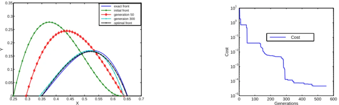
b0= (0.35, 0), b1= (0.35, 15), b2= (0.65, 0.285), b3 = (0.65, 0)

We solve the direct problem (SP ) using finite element, the obtained solution on Γ0 is then

specified as the desired temperature T0.

Fig. 2 illustrates the iterative convergence process as the initial guess for the free boundary moves towards the exact boundary Γ, for various numbers of iterations performed. From this figure, it can be seen that the numerically retrieved boundary is a very good approximation of the exact one.

(8)

5. Conclusions

This paper is concerned with the approximation of the welding problem formulated as a PDE optimization problem where the shape of the interface serves as the control variable. To avoid the shape differential calculus needed in a gradient like method for solving a shape optimization problem, we used a numerical algorithm based on genetic algorithm procedure, B´ezier curve parametrization of the free boundary and finite element discretization of the state problem. We proved the existence of the discrete optimal solution. Our computational example confirms the efficiency of the proposed approach. The convergence can be accelerated by the parallel computation procedure.

It can be stressed that the presented method admits a straightforward generalization to three dimensions. Our future work in this class of problems will involve extensions of the present method to a time-dependent problem.

0.250 0.3 0.35 0.4 0.45 0.5 0.55 0.6 0.65 0.7 0.05 0.1 0.15 0.2 0.25 0.3 0.35 X Y exact front initial front generation 50 generaion 300 optimal front 0 100 200 300 400 500 600 10−5 10−4 10−3 10−2 10−1 100 101 Generations Cost Cost

Figure 2. The cost functional decreasing. And the iterative convergence process for the unknown boundary.

References

[1] Boulkhemair A., Chakib A., On the uniform Poincar´e inequality, Comm. Partial Differential Equations, V.32, N.7-9, 2007, pp.1439-1447.

[2] Boulkhemair, A., Chakib, A., Nachaoui, A. Uniform trace theorem and application to shape optimization, Appl. Comput. Math., V.7, N.2, 2008, pp.192-205.

[3] Chenais, D. On the Existence of a Solution in a Domain Identification Problem, J. Mat. Annal. Appl., V.52, N.2, 1975, pp.189-289.

[4] Chakib, A., Ellabib, A., Nachaoui, A., Nachaoui, M. A shape optimization formulation of weld pool determination, Appl. Math. Lett., V.25, N.3, 2012, pp.374-379.

[5] Chakib, A.; Ghemires, T., Nachaoui, A. A numerical study of filtration problem in inhomogeneous dam with discontinuous permeability, Appl. Numer. Math., V.45, N.2-3, 2003, pp.123-138.

[6] Deimling, D. Nonlinear Functional Analysis, Sprenger, 1985.

[7] Holland, J. Adaptation in Natural and Artificial Systems University of Michigan Press, Ann Arbor, Mich., 1975.

[8] Haslinger, J.; Makinen, R.A.E. Introduction to Shape Optimization. Theory, Approximation, and

Compu-tation,Advances in Design and Control, 7. SIAM, Philadelphia, 2003.

[9] Ladyzenskaja, O.A; Ural’ceva, N.N. Équations aux Dérivés Partiales de Type Elliptiques,Monographies

universitaires de Math´ematiques, Dunod Paris 1968.

[10] Michalewicz, Z. Genetic Algorithms + Data Structures = Evolution Programs, Springer-Verlag, Berlin, second edition, 1994.

[11] Ciarlet, Ph.G. The Finite Element Method for Elliptic Problems, North-Holland, Amsterdam, 1978.

(9)

A. Nachaoui, for a photograph and biography, see Appl. Comput. Math., V.7, N.2, 2008, p.205.

Mourad Nachaoui _{- was born in Marrakech,}

Morocco, May 10, 1981. He received Master

and Ph.D degrees in Mathematics and scientific computing analysis from Cadi Ayyad Unversity (Marrakech (2007) and Nantes University ( France 2011), respectively.