Anticipative Control Strategy for Load Commutation of On-Board Electrical Networks

(1)

HAL Id: hal-00757772

https://hal.archives-ouvertes.fr/hal-00757772

Submitted on 27 Nov 2012

HAL is a multi-disciplinary open access

archive for the deposit and dissemination of

sci-entific research documents, whether they are

pub-lished or not. The documents may come from

teaching and research institutions in France or

abroad, or from public or private research centers.

L’archive ouverte pluridisciplinaire HAL, est

destinée au dépôt et à la diffusion de documents

scientifiques de niveau recherche, publiés ou non,

émanant des établissements d’enseignement et de

recherche français ou étrangers, des laboratoires

publics ou privés.

Anticipative Control Strategy for Load Commutation of

On-Board Electrical Networks

Pedro Neiva Kvieska, Guy Lebret, Mourad Aït-Ahmed

To cite this version:

Pedro Neiva Kvieska, Guy Lebret, Mourad Aït-Ahmed. Anticipative Control Strategy for Load

Com-mutation of On-Board Electrical Networks. International Review of Electrical Engineering, Praise

Worthy Prize, 2012, 7 (4), pp.5247-5256. �hal-00757772�

(2)

Anticipative Control Strategy for Load Commutation

of On-Board Electrical Networks

Pedro Kvieska

1

, Guy Lebret

2

, Mourad Aït-Ahmed

3

Abstract – This paper deals with the control of the output voltage of ship on-board electrical

networks when a load is connected to or disconnected from the network. In some cases this kind of disturbances can create high deviations from the nominal behavior. This includes high oscillations which can damage the network and that a classical controller cannot efficiently attenuate. The idea is to take advantage of the knowledge that an electrical device is switched on, to anticipate the disturbance. An anticipative adaptive optimal control law is tuned to create better conditions to attenuate the disturbance. Copyright © 20xx Praise Worthy Prize S.r.l. - All rights reserved.

Keywords:

Electrical Embedded Network, Optimal Control, Anticipative Control, load Commutation.

I. Introduction

In marine systems, the control of the output voltage and frequency of the electrical on-board networks are vital issues. In this particular type of networks, each load that is connected to or disconnected from the system may have an important influence over these variables. As discussed in [1], [2], for smooth load transitions and/or weakly oscillating behavior a simple fixed controller can maintain a constant output, but in abrupt situations and/or in the presence of strongly oscillating modes these controllers can reach their limits.

In this paper a strategy is proposed to adapt the control performances to the connected loads. For each load, a dedicated optimal control is used in order to respect the industrial constraints defined by the standardization agreement [3]. But the main idea is an anticipative control strategy which leads up the system to better conditions to face the load change and come back to its nominal value. For marine systems, load commutations can effectively be anticipated, since, most of the time (failure is not included here), the connection or disconnection of an electrical machine or device with high impact (crane, motor ...) comes from a switch that can also send the connection information to a controller.

Section II introduces a model of a realistic marine environment electrical network. Section III defines the considered load commutations, details the industrial control specifications found in [3] and states the control problem. The key point of anticipation is sketched in the last subsection. Section IV describes the control strategy: a two degrees of freedom architecture with an essential model based feedforward part and its finite time characteristic. The parameter tunings of this finite time optimal control law are given in section V. An example

illustrates the application of the global strategy in section VI. The final section is devoted to the conclusion.

II. Electrical model

The number of diesel generators in an electrical network of a ship can vary from two to five (sometimes more). One is always on, but when more energy is necessary the other ones can be started up. The last one is always redundant, this is a security in case of failure of the previous ones. In this study, only one generator is considered, but this not restrictive, with more than one generator the load impact would just be split but would still exist. Moreover, a closed loop control regulates the rotating speed of the diesel engine which drives the generator axis and which determined the frequency of the electrical signals. An electrical load commutation can disturb this regulation, but in this study it its considered that the rotating speed is constant. More precisely the mechanical dynamics of the engine are supposed to be decoupled from the electrical dynamics and will not be taken into account here. As a consequence, the model of the generator detailed in the subsection II.1 is the one given in [4], also based on the classical reference [5] in the domain.

Different devices (asynchronous or synchronous machines …) could be considered as loads for this generator. But in a more general point of view practical loads can be characterized by active and reactive power or equivalently by a set of resistance (R), inductance (L) and capacitance (C) characteristics. In this study, the loads which could be connected or disconnected will be defined by instantaneous variations of their R, L and C characteristics.

(3)

P. Kvieska, G. Lebret, M. Aït-Ahmed

II.1. Electrical generator machine

The electrical machine equations, in the dqframe, are [5]: Q qQ q q D dD f fd d d d s d LI M I dt dI M dt dI M dt dI L I R V = + + + −ω −ω − (1) D dD f fd d d Q qQ q q q s q LI M I M I dt dI M dt dI L I R V = + + +ω +ω +ω − (2) dt dI M dt dI M dt dI L I R V D fD d fd f f f f f = + + + (3) dt dI M dt dI M dt dI L I R VD=0= D D+ D D+ dD d + fD f (4) dt dI M dt dI L I R V_Q=0= _Q _Q+ _Q Q + _qQ q (5) where

•Id and Iq (resp. ID and IQ) are the projections of the

stator (resp. of damper windings) current in the dq frame,

•If is the excitation rotor current,

•VD = 0 and VQ = 0 in (4) and (5) since the damper

windings are short-circuited,

•Vf is the input excitation voltage,

•the output voltage is composed by its dq frame components Vd and Vq, it is given by:

3 2 2 q d out V V V = + (6)

The definition of the various parameters and their values, for simulation (section VI), are

•Nominal Power: 2.4 MW

•Nominal Frequency: 50 Hz (ω = 2π50 = 314.16 rad/s) •Nominal Output Voltage: 880 V (line to line) or 508 V

(line to ground)

•Nominal Output Current: 1875 A

•Nominal excitation voltage: 44.5 V

•Rs = 3.56 Ω : Stator Resistance •Rf = 0.155 Ω : Excitation Resistance •Ld = 2.24 mH : d-axis Inductance •Lq = 1.23 mH : q-axis Inductance •Lf = 457.9 mH : Excitation Inductance •Mfd = 29.48 mH : Mutual L d-axis/excitation •MqQ = 0.97 mH : Mutual L q-axis/damper windings •MdD = 1.9 mH : Mutual L d-axis/damper windings •MfD = 25.27 mH : Mutual L excitation/damper windings •LD = 1.9 mH : d-axis damper windings inductance •LQ = 0:97 mH : q-axis damper windings inductance •RD = 31:78 Ω : d-axis damper windings resistance •RQ = 46:19 Ω : q-axis damper windings resistance

II.2. Electrical "RLC" characterization of the loads

Loads are often characterized as RL circuits, based on active and reactive power (like in [5], [6]). Here the loads will be considered as a two-branch parallel circuit: a branch that represents the active and reactive components

of the load (RL characteristics), and a second parallel branch with a capacitance (C characteristic) that is equivalent to the negative reactive power component of the load.

For a given load L = {Rload, Lload, Cload}, the load

equations are •RL load 1 1 1 load d load q d load d L I dt dI L I R V = + −ω (7) 1 1 1 load d q load q load q L I dt dI L I R V = + +ω (8) •C load dt dV C V C Id − load q+ load d − = 2 ω 0 (9) dt dV C V C I_q + _load _d+ _load q − = 2 ω 0 (10) •currents decomposition 2 1 d d d I I I = + (11) 2 1 q q q I I I = + (12)

Note that with the introduction of this RLC load the global system presented in the next subsection has now nine states, and that Vd and Vq are now part of the state.

II.3. The global electrical network model

Considering the electrical machine equations (1) to (5), the load equations (7) to (12), the global state equations can be naturally given by the following linear descriptor system, where ω is supposed to be constant and the input control u is the excitation voltage Vf

(

R L C

)

x A

(

R L C

)

x B u E_sys _load, _load, _load, 1= _sys _load, _load, _load, + _sys (13)

with 11 1 1 1 1 1 1 1 1 1 1 1 2 3 44 4 4 4 4 4 4 4 4 4 4 4 5 6 − − − − − − − − − − − − − − − − − − − − − − = load load loas load Q qQ qQ D fD dD dD fD f fd fd qQ q q dD fd d d sys C C L L L M M L M M M M L M M M L L M M L L E 0 0 0 0 0 0 0 0 0 0 0 0 0 0 0 0 0 0 0 0 0 0 0 0 0 0 0 0 0 0 0 0 0 0 0 0 0 0 0 0 0 0 0 0 0 0 0 0 0 0 0 0 0 0 0 0 0 0 0

(4)

11 1 1 1 1 1 1 1 1 1 1 1 2 3 44 4 4 4 4 4 4 4 4 4 4 4 5 6 − − − − − − − − − = 0 0 0 0 1 0 0 0 0 0 0 0 0 0 1 0 1 0 0 0 0 0 0 0 1 0 0 0 0 0 0 0 0 0 0 0 0 0 0 0 0 0 0 0 0 0 0 0 0 0 0 0 0 0 1 0 0 0 1 0 0 load load load load load load Q D f dD fd s s q q qQ q q s s sys C C R L L R R R R M M R R L L M L L R R A ω ω ω ω ω ω ω ω ω ω ω (0 0 −1 0 0 0 0 0 0) = T sys B and

(

d d q q f D Q d q

)

T _I _I _I _I _I _I _I _V _V x = ₁ ₂ ₁ ₂

Esys(Rload, Lload, Cload) is a non-singular matrix, so this

regular descriptor system can be rewritten in a classical Linear Parameter-Varying (LPV) [7] form:

(

)

(

)

(

R L C

)

B u E x C L R A C L R E x sys load load load sys load load load sys load load load sys 1 1 , , , , , , − − + = 1 ₍₁₄₎

Finally, for a given load L = {Rload, Lload, Cload}, the

model (denoted (Σ)) which gives the output voltage as a function of the excitation voltage is defined by the following linear dynamic equation and non-linear output equation: Bu Ax x1= + (15)

( )

x h V_out= (16) with

(

load load load

)

sys

(

)

sys R L C A R L C

E

A= , , −1 , ,

(

)

sys

sys R L C B E B= , , −1 and

( )

3 2 9 2 8 x x x h = + (17)

Note that the output voltage is a function of the two states x8=Vdand x9=Vq. So the output voltage will always be continuous, even during commutation. This was, of course, physically expected from a circuit with such capacitive components.

III. Definitions of the Commutation and of

the Control Problem

III.1. Commutation definition

In this paper only instantaneous commutations are considered. The network commutes instantaneously from one load L1 = {Rload1, Lload1, Cload1} to a new load L2 =

{Rload2, Lload2, Cload2}. Moreover the network is supposed

to be in steady state before the commutation happens, with state values denoted xss1 (steady state values of the

state before the commutation). Considering the model introduced in the previous section, this means that, at time t = tc, time of commutation, the network should

commute from a model Σ1

( )

7 8 9 = + = Σ ) ( 1 1 1 _V _h _x u B x A x out 1 ₍₁₈₎

with the steady state value of the state equals to xss1, to a

new model Σ2

( )

7 8 9 = + = Σ ) ( 2 2 2 _V _h _x u B x A x out 1 ₍₁₉₎

with initial conditions equal to xss1.

Thus, after the commutation, the response of the linear dynamic part of the system is the classical sum of two responses: the response to the input of the system and the impulse response to the new initial conditions of the states. These initial conditions are equal to xss1.

Σ2 may contain natural modes of different nature. [2]

or [8] describe the possible behaviors for electrical network depending on possible realistic values of the loads: some loads lead to first order type behavior (one dominant mode), others lead to high oscillating behavior (close to imaginary axis eigenvalues with high imaginary part). So depending on the loads and also on the value of

xss1 such modes will or will not be excited. The goal of

the control u(t) is to ensure that the output voltage comes back to its nominal value, as fast as possible. So it has to change the natural modes of Σ2, make it faster if the

dominant modes are too slow, attenuate the oscillations in case of close to imaginary axis dominant eigenvalues.

III.2. Definition of the control problem

The aim of this section is to describe the control problem, based on the industrial constraints defined in [3], and to give an overview of the strategy described in sections IV and V.

A.Control specifications

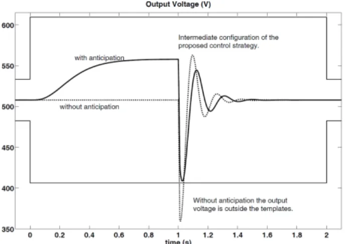
For the safety of the network during the previous defined commutation, specifications like physical limits must be respected. For this problem, [3] gives precise control specifications (figure 1 gives a graphical idea of theses constraints)

S1- The output voltage should not go over 1.05 times or under 0.95 times its nominal value during normal behavior, that is before or after a commutation. For the model of section II, the nominal value is 508 V , so 482.6 V 1 Vout 1 533.4 V.

S2- The controller has to respond to a commutation within 2 seconds after the connection request.

(5)

positive and should not go over 10 times its nominal value during load changes. For the model of section II, the nominal excitation voltage is 44.5 V , so 0 1 Vf 1 445

V.

S4- Output voltage should not go over 1.20 times or under 0.80 times its nominal value during load changes (406.4 V 1 Vout 1 609.6 V for the model of section II), or

at least if this constraint is not fulfilled, this should happen only during a "very brief" period, less than 1ms, and in this case the output voltage should not go over 5 times its steady state value (Vout 1 2540 V for the model

of section II),

S5- The output current should not go over 10 times its nominal value during load changes (less than 18750 A, for the model of section II).

Fig. 1.Output voltage during load commutation, without anticipation (dotted plot) or with anticipation (solid plot).

B.An overview of the proposed anticipative strategy

As defined in the subsection III.1, a load impact is modeled by the commutation from Σ1 to Σ2 with initial

conditions xss1. Classical approaches consider that this

load impact is an unmeasurable and uncontrollable impulse disturbance with weight xss1. In this case, H2 controllers [1] and even PID type controllers are sufficient when the load impact comes from (R, L) type loads. However, there is a class of systems ([2] or [8]), essentially due to the capacitive property of the loads, for which a more refined strategy is needed. These are the systems with high oscillating and/or with weakly controllable modes.

The dotted plot of figure 1 illustrates the typical problem that arises with such loads and controllers. If the constraint on the control signal is strictly respected, it is impossible to keep the output voltage inside the templates.

The proposed idea here is to change the steady state output voltage of the network just before the

commutation. Indeed, in marine systems load

commutations with high impact (crane, motor for anchors …) can be anticipated, since most of the time the connection of an electrical device comes from a switch

that can also send the information to a controller. This introduces a new degree of freedom in the search of an acceptable come back to the nominal voltage. As illustrated by the continuous plot of figure 1 the commutation procedure is divided in two periods, before and after the commutation. During the first period the system is driven to an intermediate configuration (or state). Section V will describe how to obtain the intermediate state value (subsection V.1). During the second period, the output voltage has to come back to its original nominal value (508 V for the example of figure 1). In both periods, a desired point has to be reached in one second: the intermediate point for the first period, the steady state of the state of Σ2 which gives the desired

nominal output voltage, during the second period. The control law strategy used for that is described in section IV. The controller topology (feedforward and feedback parts) is first described in subsection IV.1. Then the control law expression is given in subsection IV.2, this is a linear optimal finite time control law. The tunings are different for each period, they are detailed in subsection V.2.

IV. The control strategy architecture

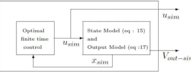
The hypotheses in this section are that equation (13) is a precise representation of the dynamic behavior of the network. So the control law design can be based on the model (15,16). The output equation (16) (or 17) is nonlinear but the dynamic state equation (15) is linear. Subsection IV.1 introduces the proposed control topology, a two degrees of freedom controller (figure 2) with an essential feedforward part (based on the hypothesis of known model and the linear characteristic of the dynamic equation) and a feedback part (which will regulate the difference between the model and the actual behavior). Subsection IV.2 details the feedforward part of the controller. Subsection IV.3 is devoted to the stability properties of the closed loop simulated in the feedforward block.

IV.1. The control topology

The global topology of the proposed two degrees of freedom controller is shown in figure 2.

Fig. 2. The global control topology

The feedforward controller is introduced for tracking purpose. It will generate an ideal open loop control that

(6)

should drive the system to the intermediate configuration during the first period and to the state of the nominal behavior during the second period.

A.The feedforward controller

The constraints here is to drive the state in finite time to these points and to modified the modes of the linear dynamic equation. The chosen solution is the linear finite time optimal control designed on the state model (15) which is detailed in subsection IV.2. The closed loop of this finite time control on the state model is simulated in the feedforward block. The generated control is the open loop control usim of figures 2 and 3.

Fig. 3. The "Feedforward Model Based Controller" block

Clearly the output equation (17) is absolutely not necessary for the control law design of usim. Indeed to

drive the simulated state in finite time and to control the modes of (15) a linear optimal control is enough. However, for the global control strategy, a simulation of the output (Vout-sim on figures 2 and 3) is performed to

regulate the actual electrical network output (Vout) around

this desired output.

B.The Feedback controller

The feedback controller would be useless if the idea of perfect model were true: in this case the difference between Vout-sim and Vout would be equal to zero. In fact,

unavoidable error between the model and the actual plant, considered as disturbance, among all other physical ones, will exist and should be attenuated by a feedback controller. It can be any type of controller designed on a linearized version of (15, 16) around the trajectory defined by (usim, Vout-sim). In this study it has been chosen

as a simple PID controller.

C. Commutation consideration

Since only anticipated commutations are considered here (failure is not included) the knowledge of the commutation existence is used in the feedforward block. In the simulated loop the loads characteristics Rload, Lload

and Cload are changed at each commutation and the

parameters of the feedforward controller are updated at the same time. In this sense the proposed control law could be classified in the class of gain-scheduled control laws.

IV.2. The feedforward part of the controller

In the feedforward block, the adopted solution is a finite time optimal control derived from [9] ("the tracking problem for linear system with quadratic criteria"), or [10] ("the LQ tracking problem"). This is a time dependent state feedback controller, that can be considered to be classical even if it cannot be exactly found in any textbook or journal paper (the development to obtain it can be found in [8]).

For the linear system x1=Ax+Bu, the control

(

)

c T d T_S_t _x_t _x _R _B _K _t _u B R t u()=− −1 () ()− − −1 ()+ (20)

where S(t) and K(t) are time-varying matrices solution of:

•the differential Riccati equation:

Q S B SBR S A SA S= + T − T + −₁ −1 ₍₂₁₎

with the final condition S(t=T)=ST •and the differential equation:

K B SBR K A SBu Qx Qx SAx K1=− _d− _d+ _c− _c− T + −1 T (22)

with the final condition K(T) = 0 minimizes the objective function:

(

) (

)

(

) (

)

(

)

A

− − + − − + − − = T c T c c T c d T T d dt u t u R u t u x t x Q x t x x T x S x T x J 0 () () () () 2 1 ) ( ) ( 2 1 (23)

In the above statement,

•x(t) and u(t) are respectively the state and the input control of the system

•x(T) is the state of the system reached at t = T

•xd is the desired state to reach at t = T •xc is a constant reference value for the state

•uc is a constant reference value for the control signal •ST and R are symmetric positive definite matrices. •Q is a symmetric positive semi-definite matrix.

The main first difference between the objective function (23) and the classical one ([9], [10]) is the introduction of uc. This is a way to find a solution which

focus on the behavior of the system around a reference point (xc, uc). This explains the threshold term defined by

uc in the control solution expression (it does not exist in

the classical case). Another difference is that the feedback (R−1BTS(t)) applies here on (x(t)−x_d) whereas in the classical problem it only applies on x(t).

(7)

IV.3. Stability results

In the feedforward part of the control topology, there is a simulated linear closed loop which generates the open loop control for the generator. The stability of this simulated closed loop is considered in this paragraph. This control law is a time dependent state feedback. For both periods, the stability of this simulated closed loop is proven in appendix. Then, one can also wonder if for this simulated closed loop the overall commutation will be stable especially if high frequency commutation exists. To avoid that some commutation dynamics could destabilize the loop, the following conditions are considered.

1. Only one load commutation happens during a transient period (from t = 0 s to t = 2 s on figure 1).

2. The system should have reached a steady-state value before the beginning of the first transient period (before t = 0 s). The system is connected to the same load until t = 1 s.

3. After the commutation (t 3 1 s), the new system is connected to the same new load until equilibrium is reached once again (from t = 1 s to t = 2 s).

The second condition imposes that between the beginning of the transient period and the load commutation, the global system does not change and the previous stability property shows that the closed loop is stable. The commutation is modeled as instantaneous. After the commutation, the dynamical model can be represented as a new system, with non-zero initial conditions. The third condition imposed that this system will not change as long as the equilibrium is not reached and the previous stability property also shows that this new closed loop is stable for any initial conditions. So, as the linear simulated closed loop in the feedforward block is stable before and after the commutation and as the commutation (in the feedforward block) is considered to be instantaneous, this closed loop is stable.

V. The feedforward control law tunings

In the feedforward part of the controller, the first finite time control (before commutation) has the task to drive in at most one second the state from its steady-state value before the commutation (xss1) to some more adapted

intermediate state (xd1). Then the second finite time

control after commutation has to drive the state from xd1

to a new desired state xd2 that is naturally be chosen to be

the steady state behavior of the new system (xss2). Clearly

the major difficulty here is to choose the intermediate point (xd1).

V.1. An optimization strategy for the choice of xd1, the final desired state before the commutation

The two essential difficulties in the search of xd1are

•For the system Σ1, the state xd1 should be reached in one

second and all specifications of subsection III.2 should be fulfilled.

•For the system Σ2, the output voltage should come back

to its nominal value and for all signals, the oscillations due to the initial condition xd1 should stay inside the

templates defined by the specifications (III.2).

Note that since the linear parts of the systems Σ1 or Σ2

(see 15) are controllable (whatever are Rload, Lload and

Cload (no proof here)) there always exists a control signal

that drives the state from xss1 to xd1 in one second. And

there always exists a control input that drives the state from xd1 to xss2 during the second period. But the task

here is to find control input such that all specifications are fulfilled. The following optimization problem for which reliable and performing tools exist ([11]) has been defined for this.

The idea here comes from classical optimal control ([9], [10]). For a controllable linear system

u B x A

x1= ₁ + ₁ , the analytical expression of the control law (u*

(

t,x_ss₁,x_d₁

)

) which minimizes the control signal energy and drives the state from a initial state (xss1) to a

final state (xd1) in one second is (see [9] (the tracking

problem) or [10] p. 184)

(

)

[

1 1

]

1 ) 1 ( 1 1 1 1 * _, _, 1 ₍₁₎ 1 ss A d c t A T d ss x R B e W x e x x t u = − T − − −

where Wc(t) is the continuous reachability gramian,

defined by:

A

− − − = t A t T A t c t e BR B e d W T 0 ) ( 1 1 1 ) ( ₁ 1 ) ( τ τ τ

Given xss1, the optimization problem is to find xd1

which minimizes the maximum of the absolute value of the control signal (u*

(

t,x_ss₁,x_d₁

)

) during "period 1". The objective function is

( )

_{[ ]}

(

1 1

)

* 1 , 0 1 max , ss , d t d u t x x x f ∈ = (24)

Note that without any constraints the optimal response

is simply *₁ 1 ₁

ss A

d e x

x = , for which f(xd1) equals to 0. This

is actually the homogeneous response of the system Σ1.

The introduction of the following constraints clearly excludes this solution. Since the commutation should be as smooth as possible xd1 should be searched as an

equilibrium point of Σ1. Because xd1 is a weight of the

impulse response of Σ2 (the transition response due to

initial conditions of a linear system), it should be chosen such that the constraints S1, S4 and S5 (section III.2) are fulfilled during the second period.

(8)

( )

(

1

)

1 min _d x x f d (25) Subject to the constraints

- C1: xd1 should be an equilibrium point of Σ1.

- C2: xd1 should be such that the transition response of

Σ2 fulfilled the constraints S1, S4 and S5.

This optimization problem can be solved with classical numerical tools such as Matlab.

V.2. The complete list of tuning parameters

For the two periods, xd is the final desired state, xc and

uc are the characteristics of an equilibrium behavior

around which the system will evolve during each period. The following tunings are used:

period 1:before commutation

•xd1 is the solution of the above optimization problem •xc1 = xd1

•uc1 = ud1 (the control signal associated to xd1)

period 2:after commutation

•xd2 = xss2 (steady state after period 2 (t 3 2 s) •xc2 = xss2

•uc2 = uss2 (the control signal associated to xss2)

The weights STi , Qi, Ri (i = 1; 2) are chosen using the

very classical rules of optimal control. Qi (i = 1; 2) equal

identity, Ri (i = 1; 2) are positive real scalars. STi (i = 1; 2)

are chosen to be equal to αi

1

9x9 with αi ∈ 1+. The

resulting parameters (αi, Ri) (i = 1; 2) were more

precisely chosen to give more or less balance between the final objective (reach the final desired state) and "smooth behavior" of the output and excitation voltage during the transition response.

VI. An example

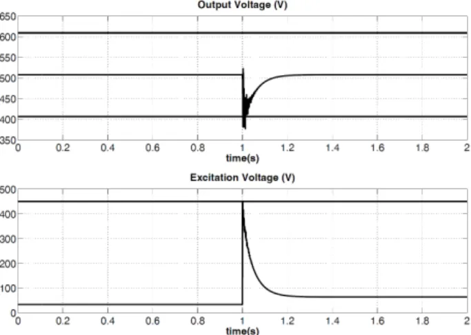
This example considers a load commutation with two very inductive loads which typically introduce some critical oscillations, critical in the sense that after commutation, the output voltage is out of the specified limits if no anticipation is used. The parameter values of the generator are the ones given in section II.1.

Before the commutation, the load and the steady state

behavior characteristics are

•Rload1 = 0.3 Ω, Lload1 = 0.8 mH, Cload1 = 1.2 mF •Active Power = 63.18 %, Power Factor = 0.84

•Vout-ss1 = 508 V, Vf-ss1 = 34.05V

After the commutation, the load and the steady state

behavior characteristics are

•Rload2 = 0.0712Ω, Lload2 = 0.563 mH, Cload2 = 1.2 mF •Active Power = 63.18 %, Power Factor = 0.40

•Vout-ss2 = 508 V, Vf-ss2 = 64.45V

Figures 4 and 6 (dotted plot on figure 6 is a zoom) show the commutation results without the anticipation during the first period, but with finite time control during the second one. Thanks to finite time control, the nominal behavior is recovered in time. Conditions S1 S2 S3 and S5 of the specifications are fulfilled. But S4 is not: the output voltage has four minima which are under the lower bound (406.4 V), two of them are associated to a time

interval greater than 1ms.

Fig. 4. Output voltage and control input if no anticipation is applied The search for an intermediate point (final desired state before the commutation) through the optimization strategy of subsection V.1 leads to a solution with the following characteristics: excitation voltage Vf-d1 = 39.47

V and output voltage Vout-d1 = 588.85 V. Figure 5 shows

the commutation results when anticipation is carried out and with finite time control during the two phases. Clearly all the conditions S1 to S5 of the specifications are now fulfilled.

Figure 6 shows a zoom of a comparison between the response without anticipation (figure 4) or with anticipation (figure 5)

Fig. 5.Response if the anticipation strategy is used, with finite control before and after commutation

(9)

anticipation (solid plot)

VII. Conclusion

This study gave a framework to the problem of load commutations for on-board marine electrical network. A commutation is defined as instantaneous changes which is equivalent to impulse disturbance. Industrial specifications have been considered to design a control law that should attenuate the effect of this disturbance (high variations including high oscillations) on the output voltage. Load commutations for which classical control is not able to respect the specifications are considered. The main idea in this study is to take advantage of the knowledge of the coming connection/disconnection of a load to anticipate the disturbance that will be created.

The controller has two degrees of freedom (feedback and feedforward). The feedback controller is a classical PID. The main contribution is in the model based feedforward control part which has been designed using the linear state equation of the model.

The major characteristics of the controller come from the feedforward part: it is an adaptive anticipative optimal controller. Anticipative, because the system is led up to better conditions to face the load change just before it effectively occurs. Adaptive, because the controller changes when the load commutes. Optimal, because to reach the intermediate point defined by the anticipation and to recover the nominal condition of operation, finite time optimal control is used in the feedforward. This strategy has been illustrated with a simulated example.

Appendix: Proof of the stability result of

subsection IV.3

This appendix proves the stability properties of the closed loop simulated in the feedforward block for each independent period (before and after the commutation). The control law (20) applied on system (15) gives

(

)

(

c

)

T d T_S _t _x_t _x _R _B _K _t _u B R B t Ax t x1()= ()− −1 () ()− + −1 ()−

which can be rewritten

(

()

)

() ()

)

(t A BR 1B S t xt g t

x1 = − − T + (26)

where g(t) is a bounded function independent of the states evolution. (26) can be considered as a Linear Parameter Varying (LPV) system [12], for which the scheduling parameter, usually called δ(t), is here δ(t) = t. Stability conditions on A_f =A−BR−1BTS(t) are given in [13] or [14]. This system is stable if there exists a square matrix P(t) such that:

0 ) (t 2 P (27) 0 ) ( ) ( ) ( ) ( 3 dt dP t A t P t P t A f T f + + (28)

Let us prove that the matrix S(t), solution of (21) is such a good candidate to prove the stability of (26).

S(t) is solution of Q S B SBR S A SA S= + T − T + −₁ −1 _{with S(T)=S} T (29) where

•Q is a symmetric positive semi-definite matrix

•R is a symmetric positive definite matrix

•ST is symmetric positive definite matrix

First of all, [15] or [16] state that S(t) is a positive definite matrix for all t, which proves condition (27).

Now, note that since S(t) and R are positive definite matrices, BTR−1B is also a definite positive matrix (B is supposed here to be full column rank). Also Q is a positive semi-definite matrix, so -Q is a negative

semi-definite matrix. From these two inequalities one obtains 0 ) ( ) (t BR 1B S t Q3 S T − − − ₍₃₀₎

Then adding (29) (or (21)) to (30) direct calculations give

(

)

(

)

(

() () () ()

)

0 ) ( ) ( ) ( ) ( 1 1 1 3 Q t S B BR t S t S A A t S t S B BR A t S t S t S B BR A T T T T T + − + − − + − − − − (31)

which is nothing else but condition (28)

0 ) ( ) ( ) ( ) ( 3 dt dS t A t S t S t A f T f + + (32)

References

[1] E. Mouni, S. Tnani, and G. Champenois, Synchronous generator output voltage real-time feedback control via H2 strategy, IEEE

(10)

Transactions on Energy Conversion, vol. 24 n. 2, June 2009, pp.

329 – 337.

[2] Pedro Neiva Kvieska, Mourad Aït-Ahmed, Guy Lebret, Gang Yao, Output voltage control of marine on-board electrical network, European Control Conference (ECC), August 24-26, 2009, Budapest, Hungary.

[3] NATO, Standardization Agreement 1008, STANAG. North

Atlantic Treaty Organization, 1994.

[4] L. Abdeljalil, Modélisation Dynamique et Commande des

Alternateurs Couplés dans un réseau électrique embarqué, Ph.D

dissertation, IREENA, Université de Nantes, Nantes, France, Novembre 2006.

[5] B. Adkins, R. G. Harley

.

The general theory of alternating current machines: Application to practical problems. (Chapman

and Hall London, 1978).

[6] L. Abdeljalil, M. Belhaj, M. Aït-Ahmed, M.F. Benkhoris. Simulation and control of electrical ship network, European

Conference on Power Electronics and Applications (EPE),

September 11-14, 2005, Dresden, Germany.

[7] F. Casella, M. Lovera, LPV/LFT modelling and identification: overview, synergies and a case study, IEEE International

Symposium on Computer-Aided Control Systems (CACSD),

September 3-5, 2008, San Antonio, Texas, USA.

[8] Pedro Neiva Kvieska, Contribution to electrical embedded

network control using Gain Scheduling techniques (in French),

Ph.D dissertation, IRCCyN, Ecole Centrale de Nantes (ECN), Nantes, France, May 2010.

[9] M. Athans, P. L. Falb, Optimal Control: An Introduction to the

Theory and Its Applications, (McGraw-Hill Book Company,

1966).

[10] Frank L. Lewis, Optimal Control, (John Wiley & Sons, 1986). [11] Jorge Nocedal, Stephen Wrigth, Numerical Optimization,

(Springer-Verlag New York Inc - 2nd Revised Edition, 2006). [12] Pedro Neiva Kvieska, Mourad Aït-Ahmed, Guy Lebret, LPV

systems: Theoretical results for gain scheduling, European

Control Conference (ECC), August 24-26, 2009, Budapest,

Hungary.

[13] Carsten Scherer, Siep Weiland, Linear Matrix Inequalities in

Control, (Delft Center for Systems and Control (DCSC) - Delft

University of Technology, 2005).

[14] Fen Wu, Control of Linear Parameter Varying Systems, Ph.D dissertation, University of California at Berkeley, USA,1995. [15] Z. Gajic, S. Koskie, C. Coumarbatch, On the singularly perturbed

matrix differential riccati equation, 44th IEEE Conference on

Decision and Control and European Control Conference ~CDC-ECC '05~, December 12-15, 2005, Sevilla, Spain.

[16] R. Wilde, P. Kokotovic, A dichotomy in linear control theory.

IEEE Transactions on Automatic Control, vol. 17 n. 3, June

1972, pp. 382 – 383.

Authors’ information

1_{P. N. Kvieska is with Technocentre Renault - Advanced Studies and}

Materials Engineering Direction. 1, avenue du Golf. 78288 Guyancourt, France (pedro.kvieska@renault.com).

2

G. Lebret is with Ecole Centrale de Nantes, IRCCyN, UMR-CNRS 6597. 1 Rue de la Noë. 44321 Nantes Cedex 03, France (guy.lebret@irccyn.ec-nantes.fr).

3

M. Aït-Ahmed is with Polytech'Nantes, IREENA, CRTT, 37 Boulevard de l'Université, BP 406. 44602 Saint-Nazaire Cedex, France (mourad.ait-ahmed@univ-nantes.fr).

Pedro Kvieska was born in Volta Redonda, Brazil,

on October 28, 1982. He received the engineer degree from State University of Campinas (UNICAMP) and Ecole Centrale Nantes in 2006. In 2010 he obtained his Doctor Degree from Ecole Centrale Nantes at IRCCyN. He now works at the Research, Advanced Studies and Materials

Engineering Direction of Renault in Paris. His main research interest lies in the control of electrical embedded networks.

Guy Lebret was born in Plancoët, Brittany,

France, on November 12, 1964. He received his Mechanical Engineering degree in 1987 and Doctor degree in Automatic Control in 1991 from the Ecole Centrale de Nantes and IRCCyN. He is currently Associate Professor at the Automatic and Robotic Department of the Ecole Centrale de Nantes and member of the control group of the research Institute IRCCyN. His main interest lies in the robust control of linear systems.

Mourad AIT-AHMED was born in Djelfa,

Algeria, on June 21, 1965. He has studied at Ecole Nationale des Ingenieurs et des Techniciens d'Algérie (ENITA), Algeria, and received the Engineer degree in electrical engineering (option Automatic) (1988). In 1993 he obtained his Doctor degree in Robotic at Université Paul Sabatier (LAAS-CNRS), Toulouse (France). He is now at the Departement of Electrical Engineering, Ecole Polytechnique de l'Université de Nantes, Saint-Nazaire, France, where he is an Associate Professor in automatic control. His main research interests are in the fields of modeling and control of electrical machines and networks.