Flood modelling improvement using automatic calibration of two dimensional river software SRH-2D

(1)

Titre: Title:

Auteurs:

Authors: Simon Deslauriers et Tew-Fik Mahdi Date: 2018

Type: Article de revue / Journal article Référence:

Citation:

Deslauriers, S. & Mahdi, T.-F. (2018). Flood modelling improvement using

automatic calibration of two dimensional river software SRH-2D. Natural Hazards,

91(2), p. 697-715. doi:10.1007/s11069-017-3150-6

Document en libre accès dans PolyPublie Open Access document in PolyPublie

URL de PolyPublie:

PolyPublie URL: https://publications.polymtl.ca/5331/

Version: Version finale avant publication / Accepted version _{Révisé par les pairs / Refereed} Conditions d’utilisation:

Document publié chez l’éditeur officiel

Document issued by the official publisher

Titre de la revue:

Journal Title: Natural Hazards (vol. 91, no 2) Maison d’édition:

Publisher: Springer URL officiel:

Official URL: https://doi.org/10.1007/s11069-017-3150-6 Mention légale:

Legal notice:

This is a post-peer-review, pre-copyedit version of an article published in Natural Hazards. The final authenticated version is available online at:

https://doi.org/10.1007/s11069-017-3150-6

Ce fichier a été téléchargé à partir de PolyPublie, le dépôt institutionnel de Polytechnique Montréal

This file has been downloaded from PolyPublie, the institutional repository of Polytechnique Montréal

(2)

1 Automatic calibration of river reach 2D simulations based on SRH-2D

1

Simon Deslauriers1_{, Tew-Fik Mahdi}2

2

1_{Département des génies Civil, Géologique et des Mines (CGM), École Polytechnique de}

3

Montréal, C.P. 6079, succursale Centre-Ville, Montréal, QC H3C 3A7, Canada. Email: 4

simon.deslauriers@polymtl.ca 5

2_{Professor, Département des génies Civil, Géologique et des Mines (CGM), École}

6

Polytechnique de Montréal, C.P. 6079, succursale Centre-Ville, Montréal, QC H3C 3A7, 7

Canada (Corresponding author). Email: tewfik.mahdi@polymtl.ca 8

Word count: 6 784 9

(3)

2 ABSTRACT

10

River model calibration is essential for reliable model prediction. The manual calibration 11

method is laborious and time consuming and requires expert knowledge. River 12

engineering software is now equipped with more complex tools that require a high 13

number of parameters as input, rendering the task of model calibration even more 14

difficult. This paper presents the calibration tool O.P.P.S. (Optimisation Program for 15

PEST and SRH-2D), then uses it in multiple calibration scenarios. O.P.P.S. combines PEST, 16

a calibration software, and SRH-2D, a bi-dimensional hydraulic and sediment model for 17

river systems, into an easy-to-use set of forms. O.P.P.S is designed to minimize the 18

user’s interaction with the involved program to carry out rapid and functional 19

calibration processes. PEST uses the Gauss-Marquardt-Lavenberg algorithm to adjust 20

the model’s parameters by minimizing an objective function containing the differences 21

between field observation and model-generated values. The tool is used to conduct 22

multiple calibration series of the modelled Ha! Ha! river in Québec, with varying 23

information content in the observation fields. A sensitivity study is also conducted to 24

assess the behaviour of the calibration process in the presence of erroneous or 25

imprecise measurements. 26

Keywords: river modelling; automatic calibration; parameter estimation; SRH-2D; PEST 27

(4)

3 1 Introduction

29

River models are used in various ways by engineers in many fields. These models are 30

relied upon to assess problems that cannot be studied directly or that are too complex 31

to be addressed via simplified approaches. River models are generally oriented towards 32

predictions in many environmentally oriented fields of study, such as water quality, 33

flood prediction and sediment transport. 34

In most study cases, the process of building a functional model comprises four main 35

steps (Vidal et al., 2007): model set-up, model calibration, model validation and 36

exploitation. Model calibration, being an essential and crucial step, consists of the 37

adjustment of the model’s parameters until a satisfactory agreement between 38

simulated values and measured values is obtained. Hydraulic models include a certain 39

variety of parameters that cannot be measured or assessed via field measurements or 40

observations. Reliable model predictions will therefore be obtained through a thorough 41

calibration process (Bahremand & De Smedt, 2010). 42

The manual calibration task is commonly performed in a trial and error process where 43

the user progressively adjusts the parameters until a satisfactory result is obtained. This 44

method is limited since the task is time consuming and the subjectivity of the quality of 45

the adjustment highly depends on the user’s experience (Boyle et al., 2000). Moreover, 46

the number of variable parameters is often reduced as much as possible by the users to 47

reduce the model’s complexity. With the ever-growing computational capabilities of the 48

(5)

4 models and the increasing demand for model precision, the manual calibration method 49

sometimes becomes inappropriate. 50

Dedicated studies have aimed to develop efficient and automatic calibration methods 51

where the parameters are adjusted until an objective function is brought to a minimum. 52

Calibration methods come in two forms: the global methods based on an evolution 53

algorithm, such as the Shuffled-Complex Evolution method (Duan et al., 1992), and the 54

gradient-based methods, such as the Gauss-Marquardt-Levenberg algorithm. Global 55

methods are robust in finding the minimum of the objective function in the entire 56

parameter space but require a great amount of model runs to achieve this result. 57

Gradient-based methods on the other hand are computationally efficient, but the result 58

can sometimes be dependent on the initial parameters as the calibration progresses 59

from an initial set of parameters towards the steepest descent of the objective function. 60

Model calibration, regardless of the chosen method , should be done with caution as 61

multiple parameter sets of model structure could exist and yield equally acceptable 62

results (Beven & Freer, 2001). The existence of these different possibilities is known as 63

“equifinality” and has been well documented before (Pathak et al., 2015). The issue of 64

equifinality is not the main focus of the authors in this study but rather the application 65

of a “work-around” technique to avoid it. 66

Though the hydraulics models have evolved into complex tools with diverse 67

functionalities to visualise and present results, calibration-oriented tools have not 68

progressed in the same manner. Additional features have been implemented in the 69

(6)

5 models to yield more capabilities in data presentation, but little has been done 70

regarding the improvement of the calibration tools: “evolution of calibration support 71

mechanisms has yet to undergo the same level of development as the models 72

themselves” (McKibbon & Mahdi, 2010). Vidal et al. (2007) depicted the same problem: 73

“even modelling packages promoting good modelling practices do not provide 74

significant features to assist users during manual calibration”. 75

For the same solver, or software, even if PEST (Parameter ESTimation) can be used to 76

calibrate a particular river model (Lavoie and Mahdi, 2016), the tedious calibration 77

process has to be repeated again for a new river model even if using the same solver. To 78

facilitate the calibration process, an automatic calibration tool is created that combines 79

PEST and SRH-2D (Sedimentation and River Hydraulics). To the knowledge of the 80

authors this is the first time that a tool based on PEST is developed to calibrate any river 81

model based on the SRH2-D, a 2D free hydrodynamics software developed by the USBR 82

(U.S. Bureau of Reclamation). The user simply specifies the parameters he wishes to 83

submit to the calibration process and the observation values to be compared with the 84

simulated results. The developed tool then assures the entire configuration and 85

execution of the calibration process. 86

The tool created is then used to explore different calibration scenarios where the effect 87

of progressively increasing the available information used by the calibration process is 88

considered. Another set of calibrations is undertaken with the introduction of an error 89

(7)

6 in the measurement values to explore the effect of erroneous data. This paper deals 90

only with the calibration of the Manning’s roughness coefficient. 91

2 Methods 92

This section introduces the hydrodynamic model used for the river reach flow 93

simulation, SRH-2D, and the optimisation program PEST. The tool developed is also 94

presented, along with the description of the conducted calibration series on the model. 95

2.1 SRH-2D 96

SRH-2D (Lai, 2008) is a depth-averaged flow and sediment transport model for river 97

systems that was developed at the U.S. Bureau of Reclamation. The software is capable 98

of simulating flow through multiple reaches, floodplains, vegetation lands and 99

hydraulics structures. SRH-2D is well suited for rivers that require a better 100

representation of 2D effects, such as multiple flow paths or in-stream structures. It 101

computes the local water elevation, local flow velocity, eddy pattern and shear stress on 102

riverbeds and banks. The software is built to easily divide rivers into different reaches 103

depending on vegetation, topography or morphology. The hybrid meshing strategy is 104

well suited to zonal modelling as it allows for both a quadrilateral and triangular shape 105

with the desired density. 106

An implicit scheme is used to solve the finite-volume numerical method based on the 2D 107

depth average dynamic wave equation of St. Venant. Steady and unsteady state can 108

both be simulated by the software, and all flow regimes may be simulated. For a better 109

understanding of the model, additional details can be found in Lai (2009), where a 110

(8)

7 complete description of the governing equation and discretisation methods is displayed. 111

Although SRH-2D is capable of computing sediment transport, this model is considered 112

static and therefore does not include aggradations or degradation of the riverbed. 113

Pre-processing and post-processing of the model is executed in SMS (Aquaveo, 2013), a 114

modelling software presented as a graphical user interface and analysis tool that holds 115

all of the SRH-2D functionalities. 116

2.2 PEST 117

To verify the reproduction of the physical phenomena by the model, the data calculated 118

by the model needs to be compared with measured values to determine the model’s 119

performance regarding the reproduction of the said phenomena. Based upon the 120

assumption that the model responds to an excitation or an impulsion, it is possible to 121

imagine that there is at least a combination of parameters that can make the model 122

reproduce the same reactions that occur in the modelled environment (Doherty, 2010). 123

PEST is a model-independent software designed to assume the task of calibration in a 124

completely automatic manner by applying the Gauss-Marquart-Levenberg algorithm 125

(Doherty, 2010). The calibration is undertaken by reducing to a minimum the objective 126

function, which holds the discrepancies between the measured values and the results 127

given by the model. PEST will gradually adjust the model parameters following the 128

steepest descent towards the minimum of the objective function until it reaches the 129

user-supplied termination criteria. The parameters obtained would hence give the best 130

match between the supplied measured values and the simulated values. 131

(9)

8 The parameter estimation is based on a linearization of the relationship between the 132

model parameters and the calculated output values. At every iteration, PEST executes as 133

many model runs as there are calibration parameters to generate their partial 134

derivatives using a user-guided finite difference. Following every model run, PEST 135

examines the output information and, based on the instruction supplied in the control 136

files, will refine the input parameters of the model towards the predicted steepest 137

descent of the objective function based on the calculation of the Jacobian matrix of the 138

model parameters. PEST will stop this process once the objective function is reduced to 139

a minimum. 140

To conduct this task, PEST takes control of the model by executing it as many times as 141

needed while modifying the parameters until the objective function is lowered to a 142

user-supplied satisfactory level. PEST requires a specific set of instructions in the form of 143

three files. The first file indicates the way in which the output information generated by 144

the model should be interrogated. The second is a mirror image of the input file, which 145

is used to locate the calibration parameters. The third file is the centre of command of 146

the whole operation and contains all the instructions regarding the calibration process 147

(Doherty, 2010). The content of these files will vary from one model to another. 148

In this unique approach, PEST is linkable to almost any type of model as long as the 149

input and output information can be accessed in any way. The sequential execution of 150

the model by PEST is accomplished via a batch file, which can be a succession of multiple 151

operations such as the translation of the output file to a readable format or the 152

(10)

9 combination of multiple information coming from the model resolution. PEST has 153

already been proven to be an effective calibration procedure for hydrological models 154

and quasi-2d hydrodynamic models (Diaz-Ramirez et al., 2012; Ellis et al., 2009; Fabio et 155

al., 2010; Kim et al., 2007; McCloskey at al., 2011; McKibbon & Mahdi, 2010; Rodeetal., 156

2007) 157

2.3 O.P.P.S. 158

The Optimisation Program by PEST for SRH-2D (O.P.P.S.) is the resulting tool for the 159

automatic calibration of SRH-2D by PEST. O.P.P.S. eases the task of preparing the 160

calibration process by correctly building the required files with the user’s desired PEST 161

regularisation parameters. O.P.P.S. comes in the form of an easy-to-use graphical 162

interface based on Excel® Visual Basic, where the user can quickly specify the current 163

project’s parameters to be calibrated and the measured values that are to be matched 164

in the model. 165

O.P.P.S can easily prepare and execute an operational PEST calibration process with 166

minimum user interaction. The model is sequentially launched by a command line in the 167

form of an AutoHotKey® file capable of conducting single model runs without any user 168

intervention. Indeed, the execution of the command lines supplied with O.P.P.S. allow 169

for carrying out the calibration process in the background without the user 170

interventions normally required by SHR-2D. A single non-calibration run would normally 171

require multiple human-directed operations that would interfere with the automatic 172

(11)

10 aspect of the calibration process. Therefore, the automatic execution of SRH-2D is made 173

completely free of user interventions. 174

When O.P.P.S. is launched, the interaction with the user is made through a series of 175

forms in which the information regarding the calibration process can be entered. A 176

summary of the procedures followed during the preparation and execution of the 177

calibration process is presented in figure 1. Any combination of measured depth, water 178

velocity along the X- and Y-axis, and the velocity magnitude at any point in the model 179

can be supplied as observation values to be compared to the simulated results for each 180

observation point. The measured values supplied are individually used in the calibration 181

process: there will be as many single observation points as there are measured values in 182

the calibration process. 183

The subsequent preparation steps are carried out by O.P.P.S. and the calibration process 184

is guided by PEST. Once the parameters and the observation points have been 185

identified, O.P.P.S can create the required files for PEST’s execution. A series of 186

verifications are performed to avoid errors or performance issues that can arise when 187

PEST is not efficiently programmed. If it does not exist already, O.P.P.S. will 188

automatically create a backup file of the project. When PEST is executed, permanent 189

changes will be applied to the selected parameters. Additional options for the fine 190

tuning of the calibration process are also available. 191

(12)

11 Additional parameters can be adjusted for the fine tuning of the calibration process by 193

managing the evolution of the calibration process.. The user can adjust the Marquardt-194

Lambda parameter, which guides the progression vector towards the optimal reduction 195

of the objective function. The progression vector is gradually reduced as PEST 196

progresses closer to the minimum of the objective function. PEST is presented with 197

multiple decision criteria that can be adjusted by the user, depending on the project at 198

hand. These criteria handle the conditions required to progress towards a new iteration 199

or to terminate the calibration process at the most appropriate moment. In both cases, 200

these regularisation parameters can be based on the evolution of the calibration 201

parameters or on the progression of the objective function. . These parameters should 202

be adjusted according to each project, as one configuration might not satisfy every 203

calibration operation. 204

2.4 Study case 205

O.P.P.S. can quickly and efficiently assemble the required information to perform an 206

operational automatic calibration process. This tool is used to perform a series of 207

calibrations of the river model.In this study, the Ha!-Ha! River is partially modelled using 208

the topographical data collected after the 1996 failure of a dam of the Ha! Ha! Lake. The 209

dam failed as water rose rapidly during the high-yield rains that lasted for three days in 210

the Saguenay region in Québec, Canada. The sudden flush caused an excessive increase 211

in the river flow (more than 1000 m3_{/s), drastically changing the river morphology by}

212

eroding the sediment deposit around the rocky bases of the riverbed. Capart et al. 213

(2007) give the cross-sections data for every 100 m of the river. 214

(13)

12 The Ha! Ha! River basin covers a total of 572 km2_{in the Saguenay-Lac-St-Jean region,}

215

and its river stretches forth a total of 35 km from the Ha!-Ha! dyke to the river mouth, 216

where it flows into the Saguenay river. The model comprises five different reaches of 217

approximately 3 km each represented by different roughness coefficients. A map of the 218

modelled reaches is presented in figure 2. The Manning roughness coefficient is the only 219

adjustable parameter in the study case as PEST only allows for the calibration of 220

continuous parameters. Although the calibration is limited to only one parameter, the 221

roughness coefficient has been identified as the most influential source of uncertainty in 222

river models (Hall et al., 2005; Warmick et al., 2010). 223

2.5 Calibration scenarios 224

The original set of parameters was established by the authors and were not 225

measurements or calculated values. The hydrodynamic results generated by running the 226

model with the original set of parameters were then used in the calibration process. 227

Using the data recorded during the initial run with the original parameters as the 228

observation values, PEST is expected to progress towards the initial set of parameters. 229

Fictional parameter values were used by the authors because not enough data for this 230

study case is available to proceed to a real calibration case. For each calibration 231

scenarios, the maximum number of iterations allowed is 30 and the parameters can 232

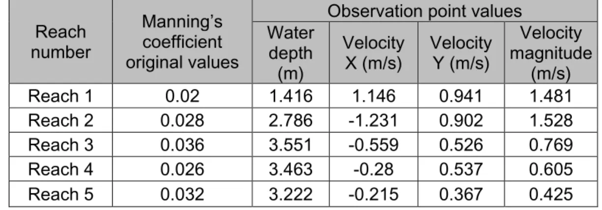
range from 0.01 to 0.1.The original values of Manning coefficients, along with the 233

observation values used in the series of calibrations, are presented in table 1. The series 234

of calibrations is carried out using different settings, with the number of observation 235

points, their positions and their content varying in each series. 236

(14)

13 The calibration was performed on a IntelCore i5 2,27 GhZ laptop and required on 237

average7 iterations and 60 model runs for the simpler cases and 10 iterations and 100 238

models runs for the more complex cases. Each model run take approximately 1 hour to 239

complete. 240

2.5.1 Water depths 241

The first series of calibrations used an increasing number of observation points, only one 242

per reach, containing only the observed water depths. In the first case, the calibration 243

points were located close to the middle of the reach; in the second case, the points 244

were located near the junctions of reaches or close to the boundary conditions. The first 245

calibration used two observation points, while the subsequent calibration used one 246

additional point, with a maximum of five (one per reach) in the first scenario and six in 247

the second scenario. 248

2.5.2 Water depths and velocities 249

The next series of calibrations also used an increasing amount of observation points 250

between each trial. In addition to water depths, observation points contained water 251

velocity measurements: water velocity in the X- and Y- directions and the magnitude of 252

this velocity. PEST now has access to an increased quantity of information to proceed 253

with the calibration to explore the extent of adding information to the observation 254

points. In all cases, the observation points are located near the centre of each reach. 255

Each calibration process is carried out with identical instructions sets and regulation 256

parameters and has the same starting values for the initial model run. 257

(15)

14 2.5.3 Sensitivity analysis

258

The next parts of the calibration series were used for a sensitivity study to observe the 259

effects of introducing an error in the measured data used in the calibration procedure. 260

Different scenarios were carried out using two different sets of observation data to aid 261

in the calibration process, with a variable magnitude of the introduced error. 262

In the first case, the error was applied to the measured depth in a scenario where only 263

the measured depth was available for the calibration procedure. In the second case, the 264

same scenario as in the previous case was carried out by adding measured velocity data 265

to the observation points to verify the advantages of additional information in the 266

advent of an error in the data. Only the measured depth was subjected to the 267

introduced error. The third case introduced an error in the model’s input flow using all 268

the available measured data of the observation points (measured depths and velocities). 269

This scenario reveals the effect of flow overestimation and underestimation on the 270

calibration. The first series of this case only included the measured depths at the 271

observation points; the second scenario included all the measured data, i.e., measured 272

depth and velocities. Again, partial use of the data in the first case was done to evaluate 273

the benefits of adding additional data to the calibration process to better handle the 274

possible introduction of error in the data. 275

3 Results and discussion 276

The results obtained in the different calibration scenarios are presented in this section, 277

and the difference between the observed and simulated water depths of the entire 278

(16)

15 model for the final calibration scenarios is shown. The results obtained from the 279

calibration series and sensitivity calibration series are also discussed. 280

3.1 Water depths 281

The first series of calibrations only used a growing number of observation points 282

containing the water depth as a means of correspondence between the model output 283

values and the measured values. At first, only two observation points were supplied; for 284

each subsequent calibration run, an observation point was added until each reach was 285

supplied with a measured water depth. Figures 3 to 6 present the calibration results 286

from the first series of calibrations. 287

Results show that PEST cannot correctly calibrate reaches without having at least one 288

observation value in the reach, which in this case is the measured water depth. In each 289

calibration process, the Manning coefficients in the reaches that are not supplied with 290

an observation point have little or no variation compared to their starting values. From 291

the observations made in the results, PEST needs to be supplied with at least one 292

measured depth in a reach to correctly estimate the parameter value. However, PEST 293

has no difficulty matching measured water depths, when supplied, in only a few model 294

runs. 295

If, during the calibration process, PEST cannot find a correlation between the variation 296

of a parameter and the reduction of the objective function, it will abandon further 297

modification of the said parameter during the present iteration. This results in 298

parameters that are left at their original values during the calibration process. Reaches 299

(17)

16 that are left with an unvaried Manning coefficient have an influence on the upstream 300

portion; thus, PEST, in its quest to match the featured values, must compensate for the 301

unvaried coefficients with an overestimation of the Manning coefficient to reach the 302

supplied measured value upstream. This is shown in the calibration results, where PEST 303

could not correctly calibrate the reach 4 parameter when no information was supplied 304

downstream in reach 3. When an observation point is added to reach 3, PEST can 305

correctly adjust the Manning coefficients of both this reach and of reach 4. 306

Figure 7 shows the differences between the water depths recorded at the end of the 307

calibration process using all the observation points and the water depths recorded with 308

the original parameter values. The differences between the simulated values are very 309

low considering that almost all the model’s water depths are reproduced within a 0.005 310

m precision. The majority of the higher differences are located in reach 2, which is an 311

area characterised by small instabilities in the results. 312

Since the low starting values of the Manning coefficient had a negative influence on the 313

calibration results, the entire calibration series is reinvestigated by reinitialising the 314

starting values in a range that would be much closer to a suitable estimation done by 315

any user. This way, the calibration process could begin with starting values that could 316

resemble a user’s estimation. 317

The results obtained show the same result pattern with a much better performance in 318

the calibration result since the starting values are closer to the original values. Like in 319

the previous series, the reaches that are not provided with calibration points remain 320

(18)

17 closer to their original values, but results show a positive movement towards the 321

desired values as more points are added. In reach 3, the relative difference between the 322

desired value and the calibration value is gradually diminished as additional points are 323

added to the surrounding reaches. The same improvement is observed at reach 4, 324

where overestimation caused by reach 3 is gradually reduced and much less 325

exaggerated, similar to the previous calibration series. 326

Another calibration series was processed by using observation points located on the 327

frontier of two reaches in the model to explore the “calibration value” of a different 328

positioning of the observation points. The results showed that points placed on the 329

frontier of two reaches facilitate only the calibration of the downstream reach; thus, 330

one point per frontier is needed to obtain a proper calibration of the model. However, 331

the uncalibrated reaches in this series did not have the overestimation effect upstream 332

observed in the previous series. 333

3.2 Water depths and velocities 334

This series of calibrations also used an increasing number of calibration points, centred 335

in their respective reaches, with additional measurements: each observation point 336

featured the measured depths, the velocity along the X- and Y-axis, and the velocity 337

magnitude. Figures 8 to 11 present the calibration results from the series of calibrations 338

using water depths and water velocities of the observation points. With only two 339

observation points (figure 8), PEST can find the desired values of 4 out of 5 reaches. The 340

calibration parameter of reach 5 remained at the starting value, meaning that PEST 341

(19)

18 could not establish a relation between the parameter variation and the reduction of the 342

objective function. 343

As additional points are included in the calibration, the relative difference between 344

PEST’s suggested values and the desired values is gradually reduced. In fact, the quality 345

of the adjustment increases faster with the addition of observation points and the 346

model is calibrated to a satisfying status with less observation points. Additionally, 347

reaches that do not have measured values to facilitate their parameter calibration can 348

be estimated to a good level when upstream and downstream reaches contain 349

calibration information. This is shown in the third calibration (figure 11), where the 350

middle reach is correctly calibrated even without having any observation values 351

attached to it. This series shows that less observation points are required to obtain 352

satisfactory calibration results when the featured points contain more information. 353

Figure 12 shows the differences between the water depths resulting from the 354

calibration process using all the observation points (water depths and water velocities) 355

and the water depths recorded with the original parameter values. The differences are 356

very similar to those of the calibration using only the water depths, with the exception 357

of reach 2, which contains the majority of the higher differences from the original 358

values. Compared to the calibrated Manning coefficient obtained in the other reaches, 359

the value from reach 2 is overestimated, thus resulting in higher but still acceptable 360

differences between the observed and simulated water depths. In the other reaches, 361

(20)

19 the differences from the simulated water depth values are still within a 0.005 m 362

precision. 363

The analysis of the results given by the hydrodynamic model shows that multiple points 364

in the reach 2 area have oscillating results over time, meaning that the final solution 365

might slightly differ from one simulation to another. The observation point used in this 366

reach was carefully selected, ensuring that the instabilities in the point’s solution were 367

limited to minor variations. It is suggested that the additional observation values 368

supplied in reach 2 were still affected by the instabilities met in the area, causing the 369

parameter overestimation. Gonzalez (2016) also denoted some numerical instabilities in 370

the modelled results. 371

Next, a sensitivity study is conducted by introducing an error in the measured values to 372

explore the effects of using erroneous measurements during the calibration process. In 373

the first calibration series, the error is embedded in the measured water depth of each 374

observation point, and the calibration process is solely based on these values to 375

approximate the parameter values. In the second calibration series, the measured water 376

velocities are added to the observation points, without any errors. In the third series, 377

the input model flow is varied and no error is introduced in the measured water depths 378

or velocities. 379

3.3 Sensitivity analysis: water depth only 380

In the case where the error is introduced in the measured water depths and the 381

calibration process relies on these values, the repercussions of the calibration error, 382

(21)

20 presented in figure 13, are distributed in a linear fashion. From the previous calibration, 383

we know that when five observation points containing measured water depths are 384

supplied, the calibration results are almost perfect. The introduction of errors in the 385

measured values raises the relative differences by a magnitude that depends on the 386

surrounding topography of the reach. Portions of the river with floodplains or larger 387

sections will suffer from more error, especially when the error overestimates the 388

measured water depth, as it will require a higher friction coefficient to match the said 389

value. Reach 1 and 2 suffer the most from the error introduction since they are the 390

portions of the river with the steepest riverbed slopes and have more floodplains. Reach 391

3 is less affected since the channel is located in a much narrower area surrounded by 392

steep hills. 393

3.4 Sensitivity analysis: water depth and speed 394

This calibration series is executed in the same manner as that of the previous one, with 395

the additions of measured water velocities to the observation points. No error is 396

introduced in these additional values. As figure 14 demonstrates, the relative 397

differences of the calibrated values are lower than those obtained in the previous series. 398

In this case, the maximum difference obtained is 20%, compared to 57% in the previous 399

situation. The differences between each parameter in the individual runs of this series 400

are less scattered, resulting in a flatter graphical display. 401

The most significant drop in relative difference between this series and the previous is 402

recorded in reach 1, where the maximum recorded value drops down from a range of 403

(22)

21 15% to 47% to an average of 2%. The considerable reduction in relative error in this 404

reach, which was previously highly sensitive to water depth variations, is the result of 405

PEST adjusting the calibration parameter by prioritising the measured water velocities 406

rather than the erroneous water depths. The results show that reaches that are more 407

oriented toward fitting the measured water velocities rather than the water depths 408

have the lowest relative error for the resulting calibrated parameter. This is shown in 409

figure 15, where calibrated parameters with a better fit towards measured water depths 410

(low relative difference between measured and calculated water depths) are more likely 411

to be miscalibrated. 412

3.5 Sensitivity analysis: discharge 413

The next series of calibrations was carried out by introducing an error in the model’s 414

input flow. Both the measured water depths and velocities were used in the calibration 415

process. Figure 16 shows the results of this series. The left side of the graph shows a 416

linear relation between error induced in the model’s input flow and error in the 417

calibration parameter. The right portion of the graph presents a much more erratic 418

relation with the flow augmentation. 419

Again, individual calibration runs that resulted in an accurate match between measured 420

and calculated water velocities at the expense of matching the measured water depths 421

are more likely to have more accurate results with the calibration of the Manning 422

coefficient. Figure 17 shows the distribution of the relative error between the 423

calibration parameters and the relative error between the observed and simulated 424

(23)

22 water depth values and water velocity values – the relative errors of water velocities are 425

summed. The Manning-water depth relation is much more concentrated on the left side 426

of the graph, with a large variation in the relative errors of the Manning coefficient. This 427

shows that when the calibration process adjusts the Manning coefficients, with a 428

tendency to match the measured water depth rather than the water velocities, the 429

calibration results are somehow more unpredictable. 430

4 Conclusion 431

This study presents the development of a tool combining PEST, an automatic calibration 432

program, with the hydraulic model SRH-2D. The tool serves as an easy-to-use set of 433

forms that can provide a rapid and functional linkage of a model with the automatic 434

calibration tool. The amount of information required by the user and the user’s 435

interaction with the tool are minimized to provide a rapid preparation of the calibration 436

process for the project at hand. 437

The tool was applied to the Ha! Ha! river model based on the post-flooding event of 438

1996, which drastically changed its morphology. The model comprised five reaches, 439

each represented by a Manning roughness coefficient. An original set of parameters was 440

used to generate observation values that were then used for multiple calibration series 441

conducted to assess the effect of different scenarios on the calibration results. The 442

positions, number and content of the observation points varied in the scenarios to 443

establish the minimal calibration conditions and common guidelines for the usage of the 444

tool. 445

(24)

23 The first series of calibrations used a growing number of observation points containing 446

the measured water depth until each section was supplied with one observation point. 447

The calibration results were optimal when one observation point was present for every 448

reach of the model. Reaches without observation points led to miscalibrated 449

parameters that negatively influenced the calibration of the upstream parameter. This 450

negative effect on the upstream reach could be corrected by using observation points 451

that are as far away as possible from the miscalibrated reach. 452

The results from another calibration series, where the measured water velocities were 453

added to the observation points, showed that fewer observation points are required to 454

yield satisfactory calibration results. The use of water velocities in the calibration 455

process, combined with the water depths, indeed proved to be much more effective 456

when estimating parameter values. Moreover, the additional information significantly 457

reduced the calibration error when slight errors were introduced in the measure water 458

depths. 459

A sensitivity analysis also showed that parameters that were calibrated by providing a 460

better fit between measured and modelled water velocities presented better results. 461

Indeed, parameters accentuating the concordance of water depths displayed a wide 462

range of errors compared to velocities based on parameters that had a more predictable 463

outcome regarding the calibration error. 464

It is suggested that the automatic aspect of the tool should be used to address the 465

question of uncertainty and equifinality associated with the parameter estimation 466

(25)

24 obtained through the calibration process. Additional scenarios should be tested to 467

explore the continuity of the model performance or the continuity of the parameter 468

estimation when the following calibration conditions are changed: parameter starting 469

values, parameter range, observation values disposition, etc. Additionally, the 470

calibration process should be revisited using different performance criteria based on a 471

global evaluation of the modelled results or a subdomain measurement of performance. 472

Pappenbergeret al. (2007) showed that the way of evaluating the model performance in 473

the calibration process (i.e., objective function) has an impact on the results at different 474

scales (local or global). Precaution must also be taken when assessing the calibration 475

process as equifinality can be encountered when multiple sets of parameters may 476

satisfy the fitting of the observation data (Beven & Freer, 2001; Pappenberger et al., 477

2005). 478

Considering the positive results obtained using the current build of O.P.P.S, further work 479

should be done to include the sediment transport module of SRH-2D in the automatic 480

calibration process. As of now, PEST does not include the calibration of discontinuous 481

parameters, which could possibly cause problems considering that sediment transport 482

parameters include integer-like input values. In this case, the calibration could be 483

executed in two consecutive motions: the first would calibrate the continuous 484

parameters; the second, using the calibration results of the continuous parameters, 485

could iterate through a user-selected range of discontinuous parameters, selecting the 486

set of parameters giving the best fit. 487

(26)

25 Acknowledgments

488

This research was supported in part by a National Science and Engineering Research 489

Council (NSERC) Discovery Grant, application No: RGPIN-2016-06413. 490

(27)

26 References

492

Aquaveo. (2013). SMS User Manual, Surface-water Modeling System (v11.1). 493

Bahremand, A., & De Smedt, F. (2010). Predictive Analysis and Simulation Uncertainty of 494

a Distributed Hydrological Model. Water Resources Management, 24(12), 2869-495

2880. doi:10.1007/s11269-010-9584-1 496

Beven, K., & Freer, J. (2001). Equifinality, data assimilation, and uncertainty estimation 497

in mechanistic modelling of complex environmental systems using the GLUE 498

methodology. Journal of Hydrology, 249(1), 11-29. 499

Boyle, D. P., Gupta, H. V., & Sorooshian, S. (2000). Toward improved calibration of 500

hydrologic models: Combining the strengths of manual and automatic methods. 501

Water Resources Research, 36(12), 3663-3674.

502

Capart, H., Spinewine, B., Yougn, D. L., Zech, Y., Brooks, G. R., Leclerc, M., & Secretan, Y. 503

(2007). The 1996 Lake Ha! Ha! breakout flood, Quebec: Test data for geomorphic 504

flood routing methods. Journal of Hydraulic Research, 45, 97-109. 505

Diaz-Ramirez, J. N., McAnally, W. H., & Martin, J. L. (2012). Sensitivity of Simulating 506

Hydrologic Processes to Gauge and Radar Rainfall Data in Subtropical Coastal 507

Catchments. Water Resources Management, 26(12), 3515-3538. 508

doi:10.1007/s11269-012-0088-z 509

Doherty, J. (2010). PEST, Model-Independant Parameter Estimation User Manuel : 5th 510

Edition: Watermark Numerical Computing.

511

Duan, Q., Sorooshian, S., & Gupta, V. (1992). Effective and efficient global optimization 512

for conceptual rainfall-runoff models. Water Resour. Res, 28(4), 1015-1031. 513

Ellis, R. J., Doherty, J., Searle, R. D., & Moodie, K. (2009). Applying PEST (Parameter 514

ESTimation) to improve parameter estimation and uncertainty analysis in

515

WaterCAST models. Paper presented at the 18th World IMACS Congress and

516

MODSIM09 International Congress on Modelling and Simulation: Interfacing 517

Modelling and Simulation with Mathematical and Computational Sciences, Cains, 518

Australia. http://mssanz.org.au/modsim09

519

Fabio, P., Aronica, G. T., & Apel, H. (2010). Towards automatic calibration of 2-D flood 520

propagation models. Hydrology and Earth System Sciences, 14(6), 911-924. 521

doi:10.5194/hess-14-911-2010 522

Gonzalez, P. (2016). Modélisation de la propagation des inondations en zone urbaine. 523

(Master), Université de Montréal, École Polytechnique de Montréal. 524

Hall, J. W., Tarantola, S., Bates, P. D., & Horritt, M. (2005). Distributed Sensitivity 525

Analysis of Flood Inundation Model Calibration. Journal of Hydraulic Engineering, 526

131(2), 117-126. doi:10.1061/(ASCE)0733-9429(2005)131:2(117)

527

Kim, S. M., Benham, B. L., Brannan, K. M., Zeckoski, R. W., & Doherty, J. (2007). 528

Comparison of hydrologic calibration of HSPF using automatic and manual 529

methods. Water Resources Research, 43(1), n/a-n/a. doi:10.1029/2006wr004883 530

Lai, Y. G. (2008). SRH-2D version 2: Theory and User’s Manuel: U.S. Department of the 531

Interior Bureau of Reclamation Technical Service Center Denver, Colorado. 532

Lai, Y. G. (2009). Two-dimensional depth-averaged flow modeling with an unstructured 533

hybrid mesh. Journal of Hydraulic Engineering, 136(1), 12-23. 534

(28)

27 Lavoie, B., & Mahdi T.-F. (2016). Comparison of two-dimensional flood propagation 535

models: SRH-2D and Hydro_AS-2D. Natural Hazards, 86(3), 1207-1222. 536

doi:10.1007/s11069-016-2737-7 537

McCloskey, G., Ellis, R., Waters, D., & Stewart, J. (2011). PEST hydrology calibration 538

process for source catchments–applied to the Great Barrier Reef, Queensland.

539

Paper presented at the 19th International Congress on Modeling and Simulation, 540

Perth, Australia. 541

McKibbon, J., & Mahdi, T. -F. (2010). Automatic calibration tool for river models based 542

on the MHYSER software. Natural Hazards, 54(3), 879-899. doi:10.1007/s11069-543

010-9512-y 544

Pappenberger, F., Beven, K., Frodsham, K., Romanowicz, R., & Matgen, P. (2007). 545

Grasping the unavoidable subjectivity in calibration of flood inundation models: 546

A vulnerability weighted approach. Journal of Hydrology, 333(2), 275-287. 547

Pappenberger, F., Beven, K., Horritt, M., & Blazkova, S. (2005). Uncertainty in the 548

calibration of effective roughness parameters in HEC-RAS using inundation and 549

downstream level observations. Journal of Hydrology, 302(1-4), 46-69. 550

doi:10.1016/j.jhydrol.2004.06.036 551

Pathak, C. S., Teegavarapu, R. S., Olson, C., Singh, A., Lal, A. W., Polatel, C., . . . Senarath, 552

S. U. (2015). Uncertainty analyses in hydrologic/hydraulic modeling: Challenges 553

and proposed resolutions. Journal of Hydrologic Engineering, 20(10), 02515003. 554

Rode, M., Suhr, U., & Wriedt, G. (2007). Multi-objective calibration of a river water 555

quality model—Information content of calibration data. Ecological Modelling, 556

204(1), 129-142.

557

Vidal, J. P., Moisan, S., Faure, J. B., & Dartus, D. (2007). River model calibration, from 558

guidelines to operational support tools. Environmental Modelling & Software, 559

22(11), 1628-1640. doi:10.1016/j.envost.2006.12.003

560

Warmick, J. J., Klis, H. v. d., & Hulscher, M. J. B. S. J. M. H. (2010). Quantification of 561

uncertainties in a 2 D hydraulic model for the Dutch river Rhine using expert

562

opinions. Paper presented at the Environmental Hydraulics.

563 564

(29)

28 Figures Captions

566

Fig O.P.P.S. flow chart 567

Fig 2 Ha!-Ha! river map and model overview 568

Fig 3 Calibration results using water depths - 2 observation points 569

Fig 7 Overall water depths differences between original values and calibrated results 573

using 5 observation points 574

Fig 8 Calibration results using water depths and water velocities - 2 observation points 575

using 5 observation points containing water depths and velocities 580

Fig 13 Calibration sensitivity against measured water depths only 581

Fig 14 Calibration sensitivity against measured water depths with additional information 582

to the observation points 583

(30)

29 Fig 15 Calibration error distribution of calculated water depth error and the summed 584

error of calculated water velocities 585

Fig 16 Calibration sensitivity against model input flow using measured water depth and 586

velocities 587

Fig 17 Calibration error distribution of calculated water depth error and the summed 588

(31)

30 Tables

591

Table 1 Original values of the Manning coefficient and observation values 592 Reach number Manning’s coefficient original values

Observation point values Water depth (m) Velocity X (m/s) Velocity Y (m/s) Velocity magnitude (m/s) Reach 1 0.02 1.416 1.146 0.941 1.481 Reach 2 0.028 2.786 -1.231 0.902 1.528 Reach 3 0.036 3.551 -0.559 0.526 0.769 Reach 4 0.026 3.463 -0.28 0.537 0.605 Reach 5 0.032 3.222 -0.215 0.367 0.425 593 594

(32)

31 595

(33)

32 596

(34)

33 597

(35)

34 598

(36)

35 599

using 5 observation points 601

(37)

36 602

(38)

37 603

(39)

38 604

using 5 observation points containing water depths and velocities 606

(40)

39 607

608

609 610

(41)

40 611

614

615 616

(42)

41 617