Exhaustive analysis of dynamical properties of Biological Regulatory Networks with Answer Set Programming

HAL Id: hal-01252610

https://hal.archives-ouvertes.fr/hal-01252610

Submitted on 17 May 2016

HAL is a multi-disciplinary open access

archive for the deposit and dissemination of

sci-entific research documents, whether they are

pub-lished or not. The documents may come from

teaching and research institutions in France or

abroad, or from public or private research centers.

L’archive ouverte pluridisciplinaire HAL, est

destinée au dépôt et à la diffusion de documents

scientifiques de niveau recherche, publiés ou non,

émanant des établissements d’enseignement et de

recherche français ou étrangers, des laboratoires

publics ou privés.

Exhaustive analysis of dynamical properties of Biological

Regulatory Networks with Answer Set Programming

Emna Ben Abdallah, Maxime Folschette, Olivier Roux, Morgan Magnin

To cite this version:

Emna Ben Abdallah, Maxime Folschette, Olivier Roux, Morgan Magnin. Exhaustive analysis of

dynamical properties of Biological Regulatory Networks with Answer Set Programming. IEEE

Inter-national Conference on Bioinformatics and Biomedicine (BIBM), Nov 2015, Washington, D.C., United

States. pp.281-285, �10.1109/BIBM.2015.7359694�. �hal-01252610�

Exhaustive analysis of dynamical

properties of Biological Regulatory

Networks with Answer Set Programming

Emna Ben Abdallah

, Maxime Folschette

, Olivier Roux

and Morgan Magnin

(Institut de Recherche en Communications et Cybern´etique de Nantes), 1 rue de la No¨e, 44321 Nantes, France. Email: {emna.ben-abdallah — olivier.roux — morgan.magnin}@irccyn.ec-nantes.fr

†_{School of Electrical Engineering and Computer Science, University of Kassel, Germany.} ‡_{I3S, UMR 7271 — Universit´e de Nice-Sophia Antipolis.}

Email: maxime.folschette@unice.fr

§_{National Institute of Informatics, 2-1-2, Hitotsubashi, Chiyoda-ku, Tokyo 101-8430, Japan.}

Abstract—The combination of numerous simple influences between the components of a Biological Regulatory Network (BRN) often leads to behaviors that cannot be grasped intuitively. They thus call for the development of proper mathematical methods to delineate their dynamical properties. As a conse-quence, formal methods and computer tools for the modeling and simulation of BRNs become essential. Our recently introduced discrete formalism called the Process Hitting (PH), a restriction of synchronous automata networks, is notably suitable to such study. In this paper, we propose a new logical approach to perform model-checking of dynamical properties of BRNs modeled in PH. Our work here focuses on state reachability properties on the one hand, and on the identification of fixed points on the other hand. The originality of our model-checking approach relies in the exhaustive enumeration of all possible simulations verifying the dynamical properties thanks to the use of Answer Set Programming.

I. INTRODUCTION

This paper is motivated by the two specific – although widespread – problems of steady states identification and reachability checking in Biological Regulatory Networks (BRNs) that describe genes and proteins interactions. Indeed, the regulatory phenomena play a crucial role in biological systems, and they need to be studied accurately. The study of BRNs has consequently been the subject of numerous researches [1], [2]. BRNs consist in sets of either positive or negative mutual interactions between the components. With the purpose of analyzing these systems, they are often modeled as graphs which makes it possible to determine the possible evo-lutions of all the interacting components of the system. Thus, in order to address the formal checking of dynamical properties within very large BRNs, new formalisms and conversely new techniques have been proposed during the last decade. For example, Boolean networks [3] have been widely used and studied due to their simplicity and ability to handle noisy data. But multi-valued discrete networks are now preferred due to their higher modeling power.

The original aim of discrete networks [4], [5] was to by-pass the complexity of continuous differential equation-based

modeling. However, these discrete representations quickly gain in complexity – in order to represent more complex behaviors or dynamical constraints – and in popularity – leading to the creation of models with thousands of components, or even dedicated databases. As more complex models arise, the need to study them is also confronted to the increasing complexity of such analyses that are usually exponential with classical model checking methods [6].

In order to address the formal checking of dynamical properties within very large BRNs, a new discrete formalism, named Process Hitting (PH) [7], was recently proposed to model concurrent systems having components with few quali-tative levels. A PH describes, in an atomic manner, the possible evolutions of a “process” (representing one component at one level) triggered by the hit of other “processes” in the system. Compared with other BRNs formalisms, the particular structure of the PH makes the formal analysis of BRNs with hundreds of components tractable [8].

Our goal in this paper is to develop exhaustive methods to analyze Biological Regulatory Networks modeled in Process Hitting. With respect to PH dynamics, this analysis consists in three kinds of results:

- Finding all possible steady states of a BRN, - Simulating the evolution of a biological network, - Computing the shortest execution path to reach a goal.

The particularity of our contribution relies in the use of Answer Set Programming (ASP) [9] to compute the results. This declarative programming framework has proved efficient to tackle models with a large number of components and parameters. Our aim here is to assess its potential w.r.t. the computation of some dynamical properties of PH models. We chose the PH framework because it allows to represent a wide range of dynamical models, and the particular form of its actions can be easily represented using ASP, with exactly one fact per action.

II. PRELIMINARY DEFINITIONS

A. Process Hitting

Definition 1 introduces the Process Hitting (PH) [7] which allows to model a finite number of local levels, called processes, grouped into a finite set of components, called sorts. A process is noted ai, where a is the sort’s name, and i is

the process identifier within sort a. At any time, exactly one process of each sort is active, and the set of active processes is called a state.

The concurrent interactions between processes are defined by a set of actions. Each action is responsible for the replace-ment of one process by another of the same sort conditioned by the presence of at most one other process in the current state. An action is denoted by ai → bj  bk, which is read

as “ai hits bj to make it bounce to bk”, where ai, bj, bk are

processes of sorts a and b, called respectively hitter, target and bounce of the action. We also call a self-hit any action whose hitter and target sorts are the same, that is, of the form: ai→ ai  ak.

The PH is therefore a restriction of synchronous automata networks, where each transition changes the local state of exactly one automaton, and is triggered by the local states of at most two distinct automata. This restriction on the actions was chosen to permit the development of efficient static analysis methods based on abstract interpretation [8]. However, despite this, we can add non-biological components into the system, called cooperative sorts, that allow to model the cooperation between 2 or more components. This allows to partly palliate the reduced expressivity of the PH framework.

Definition 1 (Process Hitting): A Process Hitting is a triple (Σ, L, H) where:

• Σ = {a, b, . . . } is the finite set of sorts; • L = Q

a∈ΣLa is the set of states where La =

{a0, . . . , ala} is the finite set of processes of sort a ∈ Σ

and la is a positive integer, with a 6= b ⇒ La∩ Lb = ∅;

• H = {ai → bj  bk ∈ La × L2b | (a, b) ∈ Σ2∧ bj 6=

bk∧ a = b ⇒ ai= bj} is the finite set of actions.

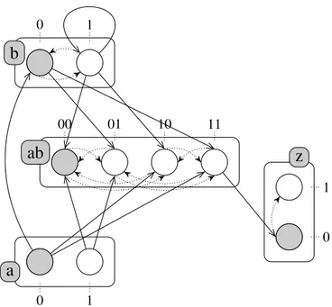
Example 1: Figure 1 represents a PH model with four sorts: a, b, z and a cooperative sort ab.

A state of the network is a set of active processes contain-ing a scontain-ingle process of each sort. The active process of a given sort a ∈ Σ in a state s ∈ L is noted s[a]. For any given process ai we also note: ai∈ s if and only if s[a] = ai. It means that

the biological component a is in the condition labeled i within state s.

Definition 2 (Playable action): Let PH = (Σ, L, H) be a Process Hitting and s ∈ L a state of PH. We say that the action h = ai → bj  bk ∈ H is playable in state s if and

only if ai ∈ s and bj ∈ s (i.e., s[a] = ai and s[b] = bj).

The resulting state after playing h in s is called a successor of s and is denoted by (s · h), where (s · h)[b] = bk and

∀c ∈ Σ, c 6= b ⇒ (s · h)[c] = s[c]. B. Dynamical properties

The study of the dynamics of biological networks was the focus of many works, explaining the diversity of network

mod-a

b

z

ab

Figure 1. An example of PH model with four sorts: a, b, ab and z. Boxes represent the sorts (biological components and logic gates), circles represent the processes (component levels), and the actions that model the dynamic behavior are depicted by pairs of arrows in solid and dotted lines. a, b and z are all either at level 0 or 1, and the cooperative sort ab has 4 levels corresponding to the combination of the levels of sorts a and b. The grayed processes stand for the possible initial state ha0, b0, ab00, z0i.

elings and the different methods developed in order to check dynamical properties. In this paper we focus on two main properties of a PH model: the stable states and the reachability. In the following, we consider a PH model PH = (Σ, L, H), and we formally define these properties. How to verify them with the help of ASP is the subject of the rest of this paper.

A fixed point, also called stable state, is a state which has no successor, as given in Definition 3. Such states have a particular interest as they denote states in which the model stays indefinitely, and the existence of several of these states denotes a switch in the dynamics [10].

Definition 3 (Fixed point): A state s ∈ L is called a fixed point (or equivalently stable state) if and only if it has no successors. In other words, s is a fixed point if and only if no action is playable in this state:

∀ai → bj  bk∈ H, ai ∈ s ∨ b/ j∈ s ./

A finer and more interesting dynamical property consists in the notion of reachability. Such a property, formally expressed in Definition 4, states that starting from a given initial state, it is possible to reach a given goal, that is, a state that contains a process or a set of processes. Checking such a dynamical property is considered difficult as, in usual model-checking techniques, it is required to build (a part of) the state graph, which has an exponential complexity.

In the following, if s ∈ L is a state, we call scenario in s any sequence of successively playable actions in s. We also note Sce(s) the set of all scenarios in s. Moreover, we denote by Proc =S

Definition 4 (Reachability property): If s ∈ L is a state and A ⊆ Proc is a set of processes, we denote by P(s, A) the following reachability property:

P(s, A) ≡ ∃δ ∈ Sce(s), ∀ai∈ A, (s · δ)[a] = ai .

The aim of this paper is to focus on the resolution of issues related to the previous definitions: we give algorithms enumerating all fixed points (Section IV) and verifying a reachability property (Section V). This last approach also requires to tackle the simulation of a PH model, that is, the enumeration of all reachable states.

III. ANSWERSETPROGRAMMING

In this section, we briefly recapitulate the basic elements of Answer Set Programming (ASP) [9], a declarative language that proved efficient to address search problems. An answer set program is a finite set of rules of the form:

a0 ← a1, . . . , am, not am+1, . . . , not an (1)

where n ≥ m ≥ 0, a0 is a propositional atom or ⊥, all

a1, . . . , an are propositional atoms, and the symbol “not”

denotes negation as failure. The intuitive reading of such a rule is that whenever a1, . . . , amare known to be true and there is

no evidence for any of the negated atoms am+1, . . . , an to be

true, then a0 has to be true as well. If a0= ⊥, then the rule

becomes a constraint (in which case a0is usually omitted). As

⊥ can never become true, if the right-hand side of a constraint is validated, it invalidates the whole answer set.

In the ASP paradigm, the search of solutions consists in computing the answer sets of a given program. An answer set for a program is defined by Gelfond and Lifschitz [11] as follows. An interpretation I is a finite set of propositional atoms. A rule r as given in (1) is true under I if and only if: {a1, . . . , am} ⊆ I ∧ {am+1, . . . , an} ∩ I = ∅ ⇒ a0∈ I .

An interpretation I is a model of a program P if each rule r ∈ P is true under I. Finally, I is an answer set of P if I is a minimal (in terms of inclusion) model of PI, where PI is defined as the program that results from P by deleting all rules that contain a negated atom that appears in I, and deleting all negated atoms from the remaining rules. Programs can yield no answer set, one answer set, or several answer sets. To compute the answer sets of a given program, one needs a grounder (to remove variables from the rules) and a solver. For the present work, we used CLINGO1[12] which is a combination of both.

IV. FIXED POINT ENUMERATION

The study of basins of attraction provides an important understanding of the different behaviors of a Biological Reg-ulatory Network (BRN) [10]. Indeed, a system will always eventually end in a basin of attraction, and this may depend on biological switches or other complex phenomena. Here we focus on fixed points (also called stable states or steady states), which are basins of attraction composed of only one state.

1_{We used CLINGOversion 4.5.0: http://potassco.sourceforge.net/}

A. Process Hitting translation in ASP

Before any analysis of the network, we first need to translate it into ASP2_{. To do this we use the self-describing}

predicates sort, process and action to define the sorts, processes and actions of the network, respectively. Example 2 shows how a PH network is defined with these predicates.

Example 2 (Representation of a PH network in ASP): The representation of the PH network of Figure 1 in ASP is the following: 1process("a", 0..1). process("b", 0..1). 2process("z", 0..1). process("ab", 0..3). 3sort(X) ← process(X,_). 4action("a",0,"b",0,1). action("b",1,"b",1,0). 5action("b",0,"ab",1,0). action("b",0,"ab",3,2). 6action("b",1,"ab",0,1). action("b",0,"ab",2,3). 7action("a",0,"ab",2,0). action("a",0,"ab",3,1). 8action("a",1,"ab",0,2). action("a",1,"ab",1,3). 9action("ab",3,"z",0,1).

In lines 1–2 we create the list of processes corresponding to each sort. For example the sort a has 2 processes numbered 0 and 1; predicate “process("a", 0..1).” will in fact expand into the two following predicates:

process("a", 0). process("a", 1).

The processes of the cooperative sort ab, which represents a cooperation between the biological components a and b, have been relabeled 0, 1, 2 and 3. Line 3 enumerates every sort of the network from the previous information. In ASP, a word starting with a capital letter is a variable, and the underscore (“_”) is a placeholder for any value. Finally, all the actions of the network are defined straightforwardly in lines 4–9; for instance, the predicate “action("a",0,"b",0,1).” represents the action a0→ b0 b1.

B. Search of fixed points

The enumeration of fixed points requires to translate the definition of a stable state (given in Definition 3) into an ASP program. The first step consists of eliminating all processes involved in a self-hit; the other processes are recorded by the predicate shownProcess (lines 11–13).

11hiddenProcess(A,I) ← action(A,I,A,I,K). 12shownProcess(A,I) ← not hiddenProcess(A,I),

13 process(A,I).

Then, we have to browse all remaining processes of this graph in order to generate all possible states, that is, all possible combinations of processes by choosing only one process from each sort (lines 14–15).

141 {selectProc(A,I) : shownProcess(A,I)} 1 15 ← sort(A).

The previous lines form a cardinality rule that creates as many potential answer sets as the number of possible states to take into account. Finally, the last step consists in filtering out any state that is not a fixed point, or, in other words, eliminating 2_{All programs, including this translation and the methods described in}

the following, are available online at: https://github.com/EmnaBenAbdallah/ verification-of-dynamical-properties PH

all candidate answer sets in which an action could be played. For this, we use a constraint: any solution that satisfies the body of this constraint will be removed from the answer set. Regarding our problem, a state is eliminated if there exists an action between two selected processes (lines 16–17).

16← action(A,I,B,J,_), selectProc(A,I), 17 selectProc(B,J), A!=B.

In the end, the fixed points of the considered model are exactly the states represented in each remaining answer, described by the atoms selectProc(A,I).

Example 3 (Fixed points enumeration): The PH model of Figure 1 contains 4 sorts: a, b and z have 2 processes and ab has 4; therefore, the whole model has 2 ∗ 2 ∗ 2 ∗ 4 = 32 states (whether they can be reached or not from a given initial state). We can check that this model contains exactly 2 fixed points: hb0, a1, ab2, z0i and hb0, a1, ab2, z1i. Indeed, there is

no action between each two processes contained in this state so no execution is possible from these.

If we execute the ASP program detailed above (lines 11–17), alongside with the description of the PH model given in Example 2 (lines 1–8), we obtain two answer sets that match the expected result:

Answer 1 : selectProc(a,1), selectProc(b,0), selectProc(z,0), selectProc(ab,2) Answer 2 : selectProc(a,1), selectProc(b,0),

selectProc(z,1), selectProc(ab,2)

V. DYNAMICAL ANALYSIS

In this section, we present at first how to determine the possible behavior of a PH model after a finite number of steps with an ASP program. Then we tackle the reachability question: are there scenarios starting from a given initial state that allow to reach a given goal? If yes, we wish to obtain one of the shortest paths to reach this goal.

A. Network simulation

In the previous section, enumerating the fixed points did not require to encode the full dynamics of PH, but only a condition, as it was a static verification. In this section, we need to implement a dynamic simulation of the PH into ASP, in order to apply an exhaustive analysis to search for the paths allowing to reach the goal.

Firstly, we focus on the simulation, that is, the evolution of a model in a limited number of steps. We therefore define the predicate time(0..n) which sets the number of steps we want to play. The value of n can be arbitrarily chosen; for example, time(0..10) will compute the 11 first steps, including the initial state. Moreover, in order to specify such an initial state, we add several facts to list of all processes included in this state:

22init(activeProcess("a",0)). 23init(activeProcess("b",0)). 24init(activeProcess("ab",0)). 25init(activeProcess("z",0)).

where, for instance, “a” is the name of the sort and “0” the index of the active process.

The dynamics of a network is described by its ac-tions; therefore, identifying the future states requires to first identify the playable actions for each state. We re-mind that an action is playable in a state when both its hitter process and target process are active in this state (see Definition 2). Therefore, we define an ASP predicate playable(action(A,I,B,J,K),T)which is true when the processes AI and BJ are active at step T.

The cardinality rule of line 26 creates a set of as many predicates as there are possible simulations from the current step, thus reproducing all possible branchings in the possible simulations of the model, in the form of as many potential answer sets. It is also needed to enforce the strictly asyn-chronous dynamics which states that exactly one process can change between two steps. To remove all scenarios where two or more actions have been played between two steps, we use the constraint of line 26. Thus, the remaining sce-narios contained in the answer sets all strictly follow the asynchronous dynamics of the PH. We finally witness that sort B has been changed between steps T and T+1 with the predicate change(B,T+1) of lines 28–29.

260 {play(Act,T)} 1 ← playable(Act,T), time(T). 27← 2 {play(Act,T)}, time(T).

28change(B,T+1) ← play(action(_,_,B,_,_),T), 29 time(T).

Finally, the active processes at step T+1, thus representing the next state in the dynamics depending on the chosen bounce, can be computed straightforwardly. Indeed, this state contains one updated active process BK resulting from the predicate

play(action(_,_,B,_,K),T) (lines 30–31) as well as all the unchanged processes that correspond to the other sorts (lines 32–34). 30instate(activeProcess(B,K),T+1) ← 31 play(action(_,_,B,_,K),T), time(T). 32instate(activeProcess(B,K),T+1) ← 33 not change(B,T+1), 34 instate(activeProcess(B,K),T), time(T).

The overall result of the pieces of program presented in this subsection is an answer set containing one answer for every possible simulation in n time steps, starting from a given initial state.

B. Reachability verification

In this section, we focus on the reachability of a set of processes which corresponds to the reachability property given in Definition 4. We use the implementation computing the dynamics given in the previous section, in order to solve this reachability problem. Moreover, we first use a predicate goal to list the processes we want to reach (line 35) and one can add as many rules of this kind as there are objective processes.

35goal(activeProcess("z",1)).

The literal reached(APr, T) then checks if a given active process APr of the goal is contained in the state of step T (line 36). Otherwise, the current answer will be eliminated by

a constraint (not detailed here) which verifies that all processes of the goal are satisfied.

36reached(APr, T) ← goal(APr), instate(APr, T).

However, the limitation of the method above is that the user has to decide upstream the number of computed steps that should be sufficient to reach all the goals. It is a main disadvantage which is shared for instance by the method proposed in [13]. One solution is then to use an incremental computation mode, which is especially tackled by the in-cremental solver of CLINGO [12]. The corresponding syntax separates the program in 3 parts. The base part contains only non-incremental elements and is thus used to declare general rules that do not depend on the time steps (such as the data related to the model). The body iteration is then written in the step(t)and check(t) parts, which are computed at each incremental step. Note that the step number t is not a variable but a constant placeholder. The step(t) part comprises rules depending on the time step, and the check(t) contains constraints that stop the iteration when needed.

When using this new syntax, the obtained program is almost identical to what was presented before, except that step numbers T are replaced by the constant placeholder t. In each step t, the program computes the following predicates:

– playable actions: playable(Act,t), – chosen action to be played: play(Act,t), – possible bounces: change(B,t),

– new state: instate(activeProcess(A,I),t+1) They are computed in the step(t) part by the same way than previously, but only for the current step. The solver then com-pares its current answer sets with the t-dependent constraint given in the check(t) part. Regarding our implementation, this constraint, given in lines 37–38, simply states that all goals have to be met. If this constraint invalidates all current answer sets, the computation continues in the next iteration in order to reach a valid answer set. As soon as one or more answer sets are not filtered out by the constraint, they are returned and the computation stops.

37notReached(t) ← goal(F), not instate(F,t). 38← notReached(t), query(t).

C. Loops elimination

The iterative version of our tool will iterate indefinitely if the dynamics of a model contains a loop. To palliate this, we define the atom getNbrRepetition(X,T,t) which contains the number X of identical active processes between the current time step t and another previous step T, although we do not detail here the method to compute this value. A loop is then easily detected by comparing this value to the total number of sorts (lines 39–41), and therefore simply eliminated by the constraint of line 42.

39loop(t, T) ← getNbrRepetition(X,T,t), 40 getNbreSorts(Y), X=Y.

41noChange(t) ← loop(t, _). 42← noChange(t).

VI. CONCLUSION AND FUTURE DIRECTIONS

In this paper, we proposed a new logical approach to address some dynamical properties of Process Hitting models. The originality of our work consists in using ASP, a powerful declarative programming paradigm. Thanks to the encoding we introduced, we are not only able to tackle the enumeration of fixed points but also to check reachability properties. The major benefit of such a method is to get an exhaustive enu-meration of all corresponding paths while still being tractable for models with dozens of interacting components.

One of the perspectives of our work is to extend the set of models on which our approach could be applied. We can consider the addition of priorities or neutralizing edges, or tackle other representations, such as Thomas modeling [5]. However, the range of the analysis can also be enriched, by searching the set of initial states allowing to reach a given goal instead of the other way around, or extending the method to universal properties (like the AF operator in CTL).

ACKNOWLEDGMENT

The European Research Council has provided financial support under the European Community’s Seventh Frame-work Programme (FP7/2007–2013) / ERC grant agreement no. 259267.

REFERENCES

[1] D. Thieffry and D. Romero, “The modularity of biological regulatory networks,” Biosystems, vol. 50, no. 1, pp. 49–59, 1999.

[2] A. Shermin, M. Orgun et al., “A 2-stage approach for inferring gene reg-ulatory networks using dynamic bayesian networks,” in Bioinformatics and Biomedicine, 2009. BIBM’09. IEEE International Conference on. IEEE, 2009, pp. 166–169.

[3] S. A. Kauffman, The origins of order: Self organization and selection in evolution. Oxford university press, 1993.

[4] ——, “Metabolic stability and epigenesis in randomly constructed genetic nets,” Journal of Theoretical Biology, vol. 22, no. 3, pp. 437– 467, 1969.

[5] R. Thomas, “Boolean formalization of genetic control circuits,” Journal of Theoretical Biology, vol. 42, no. 3, pp. 563 – 585, 1973. [6] D. Harel, O. Kupferman, and M. Y. Vardi, “On the complexity of

verifying concurrent transition systems,” Information and Computation, vol. 173, no. 2, pp. 143–161, 2002.

[7] L. Paulev´e, M. Magnin, and O. Roux, “Refining dynamics of gene reg-ulatory networks in a stochastic π-calculus framework,” in Transactions on Computational Systems Biology XIII. Springer, 2011, pp. 171–191. [8] L. Paulev´e, M. Magnin, and O. Roux, “Static analysis of biological reg-ulatory networks dynamics using abstract interpretation,” Mathematical Structures in Computer Science, vol. 22, no. 04, pp. 651–685, 2012. [9] C. Baral, Knowledge representation, reasoning and declarative problem

solving. Cambridge university press, 2003.

[10] A. Wuensche, “Genomic regulation modeled as a network with basins of attraction,” in Pacific Symposium on Biocomputing, R. B. Altman, A. K. Dunker, L. Hunter, and T. E. Klien, Eds., vol. 3. World Scientific, 1998, pp. 89–102.

[11] M. Gelfond and V. Lifschitz, “The stable model semantics for logic programming,” in ICLP/SLP, 1988, pp. 1070–1080.

[12] M. Gebser, O. Sabuncu, and T. Schaub, “An incremental answer set programming based system for finite modelcomputation,” in Logics in Artificial Intelligence. Springer, 2010, pp. 169–181.

[13] A. Rocca, N. Mobilia, ´E. Fanchon, T. Ribeiro, L. Trilling, and K. Inoue, “ASP for construction and validation of regulatory biological networks,” in Logical Modeling of Biological Systems, L. F. del Cerro and K. Inoue, Eds. Wiley-ISTE, 2014, pp. 167–206.