HAL Id: hal-01721291
https://hal.archives-ouvertes.fr/hal-01721291
Submitted on 1 Mar 2018
HAL is a multi-disciplinary open access
archive for the deposit and dissemination of
sci-entific research documents, whether they are
pub-lished or not. The documents may come from
teaching and research institutions in France or
abroad, or from public or private research centers.
L’archive ouverte pluridisciplinaire HAL, est
destinée au dépôt et à la diffusion de documents
scientifiques de niveau recherche, publiés ou non,
émanant des établissements d’enseignement et de
recherche français ou étrangers, des laboratoires
publics ou privés.
Inference of Delayed Biological Regulatory Networks
from Time Series Data
Emna Ben Abdallah, Tony Ribeiro, Morgan Magnin, Olivier Roux, Katsumi
Inoue
To cite this version:
Emna Ben Abdallah, Tony Ribeiro, Morgan Magnin, Olivier Roux, Katsumi Inoue. Inference of
Delayed Biological Regulatory Networks from Time Series Data. 14th International Conference on
Computational Methods for Systems Biology (CMSB 2016), Sep 2016, Cambridge, United Kingdom.
�10.1007/978-3-319-45177-0_3�. �hal-01721291�
Networks from Time Series Data
Emna Ben Abdallah1, Tony Ribeiro1, Morgan Magnin1,2, and Olivier Roux1,
and Katsumi Inoue2
1
LUNAM Universit´e, ´Ecole Centrale de Nantes, IRCCyN UMR CNRS 6597 (Institut de Recherche en Communications et Cybern´etique de Nantes),
1 rue de la No¨e, 44321 Nantes, France.
2 National Institute of Informatics,
2-1-2, Hitotsubashi, Chiyoda-ku, Tokyo 101-8430, Japan.
Abstract. The modeling of Biological Regulatory Networks (BRNs) re-lies on background knowledge, deriving either from literature and/or the analysis of biological observations. But with the development of high-throughput data, there is a growing need for methods that automatically generate admissible models. Our research aim is to provide a logical ap-proach to infer BRNs based on given time series data and known influ-ences amoung genes. In this paper, we propose a new methodology for models expressed through a timed extension of the Automata Networks [22] (well suited for biological systems). The main purpose is to have a resulting network as consistent as possible with the observed datasets. The originality of our work consists in the integration of quantitative time delays directly in our learning approach. We show the benefits of such automatic approach on dynamical biological models, the DREAM4 datasets, a popular reverse-engineering challenge, in order to discuss the precision and the computational performances of our algorithm. Keywords: inference model, dynamic modeling, delayed biological reg-ulatory networks, automata network, time series data.
1
Introduction
With both the spread of numerical tools in every part of daily life and the devel-opment of NGS methods (New Generation Sequencing methods), like DNA mi-croarrays in biology, a large amount of time series data is now produced[18,6,8]. This means that the produced data from the experiments led on a biological system grows drastically. The newly produced data - as long as the associated noise does not raise an issue with regard to the precision and relevance of the corresponding information - can give us some new insights on the behavior of a system. This justifies the urge to design efficient methods for inference.
Reverse engineering of gene regulatory networks from expression data have been handled by various approaches [29,16,14,34]. Most of them are only static. However, other researchers are rather focusing on incorporating temporal as-pects in inference algorithms. The relevance of these various algorithms have
been recently assessed in [15]. The authors of [17] tackled the inference problem of time-delayed gene regulatory networks through Bayesian networks. As this is a complex problem, in [33], the authors propose a Time-Window-Extension Tech-nique based on time series segmentation in different successive phases. These approaches take gene expression data into account as input and generate the associated regulations. But the discrete approaches that simplify this problem by abstractions, need to determine the relevant thresholds of each gene to define its active and inactive state. Various approches have been designed to tackle the discretization problem. We can cite for example [33], in which the authors have proposed an alternative methodology that considers not a concentration level, but the way the concentration changes (in other words: the derivative of the function giving the concentration w.r.t time) in the presence/absence of one regulator. On the other hand, the major problem for modeling lies on the quality of the expression data. Indeed, noisy data may be the main origin of the errors in the inference process. Thus, the pre-processing of the biological data is crucial pertinence of the inferred relations between components. In this work, the input data is considered to be pre-processed and the result is reliable discretized time series data.
In this paper, we aim to provide a logical approach to tackle the learning of qualitative models of biological dynamic systems, like gene regulatory networks. In our context, we assume the set of interacting components as fixed and we consider the learning of the interactions between those components. As in [3], in which the authors targeted the completion of stationary Boolean networks, we suppose that the topology of the network is given, providing us the influences among each gene as background knowledge. From time series data of the evo-lution of the system, given its topology, we learn the dynamics of the system. The main originality of our work is that we address this problem in a timed setting, with quantitative delays potentially occurring between the moment an interaction activated and the moment its effect is visible.
During the past decade, there has been a growing interest for the hybrid modeling of gene regulatory networks with delays. These hybrid approaches con-sider various modeling frameworks. In [19], the authors hybridize Petri Nets: the advantage of hybrid with regard to discrete modeling lies in the possibility of capturing biological factors, e.g., the delay for the transcription of RNA poly-merase. The merits of other hybrid formalisms in biology have been studied, for instance timed automata [28], hybrid automata [2] and boolean representation [21]. Finally, in [7], the authors investigate a direct extension of the discrete Ren´e Thomas’ modeling approach by introducing quantitative delays. These delays represent the compulsory time for a gene to turn from a discrete quali-tative level to the next (or previous) one. They exhibit the advantage of such a framework for the analysis of mucus production in the bacterium Pseudomonas aeruginosa. The approach we propose in this paper inherits from this idea that some models need to capture these timing features.
2
Background
The definition and semantics of automata networks is presented in section 2.1. The enrichment of the automata networks with delays and the corresponding new semantics is presented in section 3.
2.1 Automata Network
Definition 1 introduces the Automata Network (AN) [24,23,22] as a model of finite-state machines having transitions between their local state conditioned by the state of other automata in the network. A local state of an automaton is
noted by ai, where a is the automaton identifier, and i is the expression level
within a. At any time, each automaton has exactly one active local state, and the set of active local states is called the global state of the network.
The concurrent interactions between automata are defined by a set of local
transitions. Each local transition has this form τ = ai
`
→aj, with ai, aj being
local states of an automaton a called respectively origin and destination of t and ` is a (possibly empty) set of local states of automata other than a (with at most one local state per automaton).
Notation:Given a finite state A, ℘(A) is the power set of A. Given a network
N , state(N, t) is the state of N at a time step t∈ N.
Definition 1 (Automata Network). AnAutomata Network is a triple (Σ,S, T )
where:
– Σ ={a, b, . . . } is the finite set of automata identifiers;
– For each a ∈ Σ, S(a) = {ai, . . . , aj}, is the finite set of local states of
automatona; S =Q
a∈ΣS(a) is the finite set of global states;
LS=∪a∈ΣS(a) denotes the set of all the local states.
– T = {a 7→ Ta | a ∈ Σ}, where ∀a ∈ Σ, Ta ⊂ S(a) × ℘(LS \ S(a)) × S(a) with
(ai, `, aj)∈ Ta ⇒ ai 6= aj, is the mapping from automata to their finite set
of local transitions.
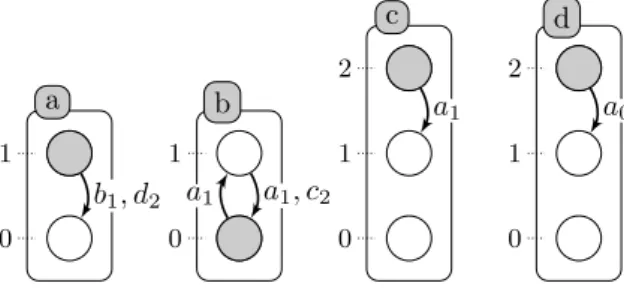
Example 1. The figure 1 represents an Automata Network, AN = (Σ, S, T )
with 4 automata (Σ = {a, b, c, d}) such that S(a) = {a0, a1}, S(b) = {b0, b1},
S(c) = {c0, c1, c2}, S(d) = {d0, d1, d2} and 5 local transitions,
T = { b0 {a1} −→b1, a1 {b1,d2} −→ a0, c2 {a1} −→c1, d2 {a0} −→d1, b1 {a1,c2} −→ b0,}.
A global state of a given AN consists in a set of all active local states of each
automaton in the network. The active local state of a given automaton a ∈ Σ
in a state ζ∈ S is noted ζ[a]. For any given local state ai we also note, ai ∈ ζ if
and only if ζ[a] = ai. For each automaton, it cannot have more than one active
local state at one global state.
Definition 2 (Playable Local Transition). Let AN = (Σ, S, T ) be an
Au-tomata Network andζ∈ S, with ζ = state(AN , t). We note Ptthe set of playable
local transitions inAN at time step t by:
Pt= { ai
`
a 0 1 b 0 1 c 0 1 2 d 0 1 2 b1, d2 a1 a1 a0 a1, c2
Fig. 1. Example of Automata Network with 4 automata: a, b, c and d presented by labeled boxes and their local states are presented by circles (for instance a is either at level 0 or 1). A local transition is a labeled directed edge between two local states within the same automaton: its label stands for the set of necessary conditions local states of the automata to play the transition. The grayed circles stand for the global state: ha1, b0, c2, d2i.
The dynamics of the AN is performed thanks to the global transitions. Indeed,
the transition from one state ζ1 to its successor ζ2 is satisfied by a set of the
playable local transitions (definition 2) at ζ1.
Definition 3 (Global Transitions). Let AN = (Σ, S, T ) be an Automata
Network and ζ1, ζ2∈ S, with ζ1 = state(AN , t) and ζ2 = state(AN , t + 1). Let
Ptbe the set of playable local transitions att. We note Gtthe power set of global
transitions att:
Gt:= ℘(Pt)
In the semantics that we are based on, parallel application of local transitions in different automata is permitted but it is not enforced. Thus the set of global
transitions is a power set of all the playable local transitions (also empty set).
3
Timed Automata Networks
In some dynamics it is crucial to have information about the delays between two events (two states of a AN ). The discrete transition, described above, cannot exhibit this information: we just process chronological information, that the state
ζ2 will be after ζ1 in the next step but it is not possible to know chronometry,
i.e., how much time this transition takes to occur and whether it blocks some transitions during this time. In fact some local transitions could not be played any more because of concurrency about shared resources (necessary components to play the transition) between them. We thus need to restrain the general dynamics to capture more realistic behavior w.r.t biology. So we propose in this section to add the delays in the local transitions attributes and give the associated semantics that we based on to infer biological networks.
Definition 4 (Timed Automata Network (T-AN)).Timed Automata
– Σ ={a, b, . . . } is the finite set of automata identifiers;
– For each a ∈ Σ, S(a) = {ai, . . . , aj}, is the finite set of local states of
automatona; S =Q
a∈ΣS(a) is the finite set of global states;
LS=∪a∈ΣS(a) denotes the set of all the local states.
– T = {a 7→ Ta | a ∈ Σ}, where ∀a ∈ Σ, Ta ⊂ S(a) × ℘(LS \ S(a)) × S(a) × N
with (ai, `, aj, δ) ∈ Ta ⇒ ai 6= aj, is the mapping from automata to their
finite set of timed local transitions.
To model biological networks where quantitative time plays a major role, we
will use T-AN (Timed Automata Network). This formalism enriches AN with
timed local transitions: ai
`
→δ aj. In the latter, δ is called a delay and represents
the time needed for the transition to be performed. When modeling a regulation phenomenon, this allows to capture the delay between the activation order of the production of the protein and its effective synthesis. and the synthesis of the product. We note ai ` →δ aj ∈ T ⇔ (ai, `, aj, δ) ∈ T (a) and ai ` → aj ∈ T ⇔ ∃δ ∈ N, ai `
→δ aj ∈ T . Given τ = ai → aj ∈ T , orig(τ) = ai, dest(τ ) = aj. Definition
2 also applies to timed local transitions.
Considering delays in the evolution of timed automata networks creates con-currency between the timed local transitions. This concon-currency is mainly justified by the shared resources between local transitions. Indeed, transitions that have the same origins and/or destinations could not be fired synchronously. Besides,
during the delay of the execution of a transition τ1, it is possible that another
transition τ2 could be activated. Then we need to take care of the following
possible conflicts between resources: transition τ2 may change the local states
of the automata participating in τ1. We make the following assumptions, that
is similar to the one adapted in [12]: we consider τ2 needs to be blocked until
the current transition τ1 finishes. Nevertheless, we allow the resources of τ1 to
participate to other transitions. In addition we do not forbid the process involved
in orig(τ1) to participate to other transition τ2if and only if that the remaining
delay(τ1) is greater than delay(τ2) (see Definition 5). Those considerations lead
to the followings definitions.
Definition 5 (Blocked Timed Local Transition). LetAN = (Σ,S, T ) be a
T-AN andt∈ N. Let P be a set of pairs T × N. The set of blocked timed local
transitions ofAN by P at t is defined as follows:
B(AN , P, t) := {ai ` → δ aj ∈ T | ∃(bk `0 → δ0 bl, t
0) ∈ P such that (a = b) ∨(a
i ∈
`0∧ δ0 > t0− (t + δ)) ∨(b
k ∈ ` ∧ δ0< t0− (t + δ))}
In definition 5, if P is the set of currently ongoing timed local transition, it al-lows us to prevent the execution of transitions that would alternate the resources currently being used or that would rely on resources that will be modified before
the end of those transitions. Let t1be a transition such that τ1= ai
`
→δ aj is fired
of time between the ending of the transition τ2= bk `
→ bl
δ0 and the beginning of
transition τ1 with t0 > t. According to the definition 5, τ2 is blocked if ai (resp.
bk) is a necessary resource for τ2 (resp. τ1) and the τ1 (resp. τ2) finishes before
τ2 (resp. τ1): δ0 > t0− (t + δ) (resp. δ0 < t0 − (t + δ)) i.e ai (resp. bk) is not
available to participate in the transition τ2 (resp. τ1) during δ0 (δ).
Definition 6 (Fireable Timed Local Transition). Let AN = (Σ, S, T ) be
a T-AN, ζ ∈ S the state of AN at t ∈ N. Let P be a set of pairs T × N
and B(AN , P, t) be the set of blocked timed local transitions of AN by P at t.
The set of fireable local transitions ofAN in ζ w.r.t. P at t is defined as follows:
F (AN , ζ, P, t) := {ai
`
→aj ∈ T \ B(AN , P, t) | ` ⊆ ζ, ai ∈ ζ}
Definition 6 extends the notion of playable transition by considering con-curencies with the currently ongoing transition of P .
Definition 7 (Set of Fireable Sets of Timed Local Transition). LetAN =
(Σ,S, T ) be a T-AN, ζ ∈ S the state of AN at t ∈ N. Let P be a set of pairs
T × N and F (AN , ζ, P, t) the set of fireable local transitions of AN in ζ w.r.t.
P at t. The set of firable sets of timed local transition ofAN in ζ w.r.t. P at t
is defined as: SF S(AN , ζ, P, t) := {F S ⊆ F (AN , ζ, P, t) | (∀τ = (bk ` →δ bl)∈ F S, @(bk `0 →δ0 bl 0)∈ F S, bl6= bl0, τ 6∈ B(AN , F S \ {τ}, t)}
Definition 7 prevents the execution of two transitions that would affect the same automaton.
Definition 8 (Active Timed Local Transitions). Let AN = (Σ, S, T ) be
a T-AN, ζ ∈ S the state of AN at t ∈ N. Let SF S(AN , ζ, P, t) be the set of
firable sets of timed local transition. The set of active timed local transitions of
AN at t is: A(AN , t) := {(τ ∈ F S, t) | F S ∈ SF S(AN , ζ, ∅, t)} if t = 0 {(τ ∈ F S, t) | F S ∈ SF S(AN , ζ, A(AN , t − 1), t)} ∪{(bk `0 →δ0 bl, t 0)∈ A(AN , t − 1) | t − t0 < δ} if t > 0
Definition 8 provides us the evolution of the possible set of ongoing actions. Supposing that in the initial state of a trajectory (at t = 0) no transition is blocked and all playable timed transitions are fireable. Then, when t > 0, at each time step it should be verified that a playable timed transition is also fireable, in other words that it is not blocked by the active timed local transitions fired in previous steps. Furthermore the timed local transitions fired at the same time should not block each other.
Delays of local transitions can now be represented in an Automata Network
set to 0 it is equivalent to an AN without delays (original AN). The way these new local transitions should be used is described as follows.
At any time, each automaton has one and only one local state, forming the
global stateof the network. Choosing arbitrary ordering between automata
iden-tifiers, the set of global states of the network is referred to as S with S =
Q
a∈ΣS(a). Given a global state ζ ∈ S, ζ(a) is the local state of automaton a
in ζ, i.e., the a-th coordinate of ζ. We write also ai ∈ ζ ⇔ ζ(a) = ai; and for
any ls ∈ LS, ls ⊂ ζ ⇔ ∀ai ∈ ζ, ζ(a) = ai. In this paper, we allow, but do not
force, applying in parallel transitions in different automata such in definition 3 but adding delays in the local transitions and considering concurrency between transitions require further study of the semantics of the model (definition 9).
Definition 9 (Semantics of Timed Automata Network ). Let AN =
(Σ,S, T ) be a T-AN and t ∈ N. The set of timed local transition fired at t
is: F S :={(ai ` →δ aj)| ((ai ` →δ aj), t)∈ A(AN , t)} then (ai `
→δ aj)∈ F S =⇒ ζ(a) = aj with ζ = state(AN , t + δ).
The state of AN at t + 1 is denoted ζt+1 = state(AN , t + 1) and defined
according to the set of timed local transitions that finished att + 1:
Ft+1:={(bk `0 → δ0 bl)| ((bk `0 → δ0 bl), t 0) ∈ A(AN , t), t + 1 − t0 = δ }
then ∀c ∈ Σ, such that @(ck
`00
→δ00 cl) ∈ Ft+1 =⇒ ζt+1(c) = ζt(c) with ζt =
state(AN , t) and ζt+1= state(AN , t + 1)
We note that at any time step t such that ζ = state(AN , t) and P the set of
ongoing transitions, we have: F S∈ F (AN , ζ, P, t) ∈ T \ B(AN , P, t).
Where synchronous biological regulatory networks have been studied, little has been done on the asynchronous counterpart [31], although there is evidence that most living systems are governed by synchronous and asynchronous up-dating. According to Harvey and Bossomaier [13], asynchronous systems are biologically more plausible for many phenomena than their synchronous coun-terpart and observed global synchronous behavior in nature usually simply arises from the local asynchronous behavior. In this paper, we defend these assump-tions and we consider an asynchronous behavior for each automata in one hand and a synchronous behavior in the global network.
The assumptions in the synchronous model that all components could change at the same time and take an equivalent amount of time in changing their expres-sion levels, is biologically unrealistic. But there is seldom enough informations to be able to discern the precise order and duration of state transitions. The timed extension of Automata Network we propose in this paper allows both asynchronous and synchronous behavior by proposing a non-deterministic ap-plication of the timed local transitions. Figure 2 shows a trajectory of a Timed
Automata Network when we choose to apply timed local transition in a syn-chronous maner.
We presented above the semantics of the T-AN that we are based on to mod-eling BRNs from experimental data. Even if it already exists a few hybrid for-malisms like time Petri Nets, hybrid automata, etc..., we propose this extension of the AN framework for several reasons. First, AN is a general framework that, although it was mainly used for biological networks [23,9], allows to represent any kind of dynamical models, and converters to several other representations are available. Indeed, a T-AN is a subclass of time Petri nets [10]. Finally, the particular form of the timed local transition in a AN model allows to easily rep-resent them in Answer Set Programming (ASP), with one fact per timed local transition, as described in this work [1]. Later we propose a new approach to resolve the generation problem of T-AN models from time series data.
Taking the following timed automata network as an example, we generate a possible trajectory of the network starting from a known initial state.
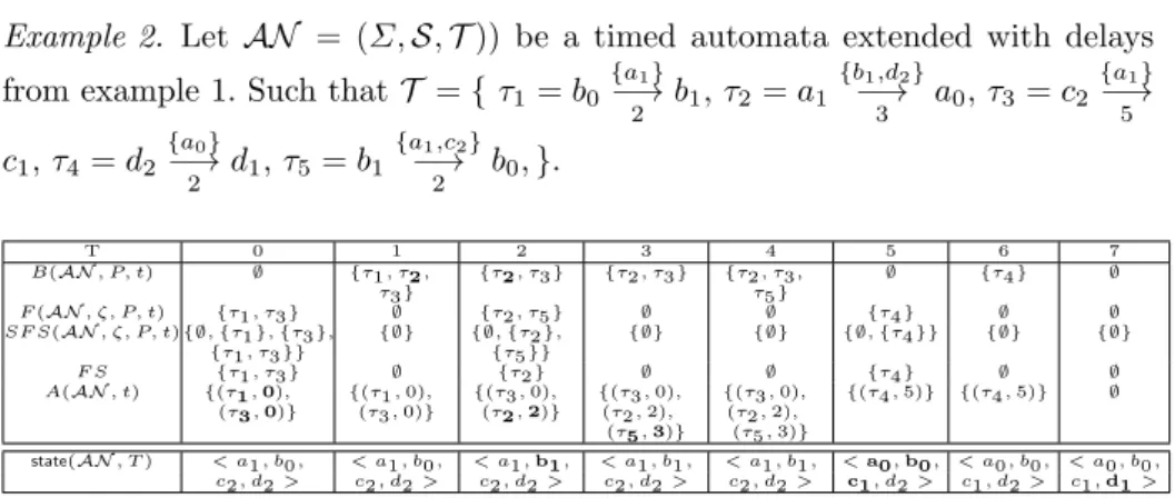
Example 2. Let AN = (Σ, S, T )) be a timed automata extended with delays
from example 1. Such thatT = { τ1= b0
{a1} −→2 b1, τ2= a1 {b1,d2} −→3 a0, τ3= c2 {a1} −→5 c1, τ4= d2 {a0} −→2 d1, τ5= b1 {a1,c2} −→2 b0,}. T 0 1 2 3 4 5 6 7 B(AN , P, t) ∅ {τ1, τ2, τ3} {τ2, τ3} {τ2, τ3} {τ2, τ3, τ5} ∅ {τ4} ∅ F (AN , ζ, P, t) {τ1, τ3} ∅ {τ2, τ5} ∅ ∅ {τ4} ∅ ∅ SF S(AN , ζ, P, t) {∅, {τ1}, {τ3}, {τ1, τ3}} {∅} {∅, {τ2}, {τ5}} {∅} {∅} {∅, {τ4}} {∅} {∅} F S {τ1, τ3} ∅ {τ2} ∅ ∅ {τ4} ∅ ∅ A(AN , t) {(τ1, 0), (τ3, 0)} {(τ1, 0),(τ3, 0)} {(τ3, 0),(τ2, 2)} {(τ3, 0),(τ2, 2), (τ5, 3)} {(τ3, 0), (τ2, 2), (τ5, 3)} {(τ4, 5)} {(τ4, 5)} ∅
state(AN , T ) < a1, b0, < a1, b0, < a1, b1, < a1, b1, < a1, b1, < a0, b0, < a0, b0, < a0, b0,
c2, d2 > c2, d2 > c2, d2 > c2, d2 > c2, d2 > c1, d2 > c1, d2 > c1, d1 >
Fig. 2. Example of a trajectory of the timed automata network of Example 2 starting from an initial state <a1, b0, c2, d2> (at t = 0) to a stable state < a0, b1, c1, d1 > (at
t = 10). With P = A(AN, t − 1) as in Definition 8.
4
Learning Timed Automata Networks
This algorithm takes as input a model expressed as a Timed Automata Network, which the set of local transitions is empty, and time series data capturing the dynamics of the studied system. Given the influences between the components (or assuming all possible influences if no background knowledge is available), this algorithm generates the timed local transitions that could result in the the same changes of the model than the ones observed through the observation data.
4.1 Algorithm
In this section we propose an algorithm to build Timed Automata Networks from time series data. We assume that the latter data observations are provided
as a chronogram of size T : the value of each variable is given for each time point
t, 0≤ t ≤ T , through a time interval discretization (see Definition 10 below).
Definition 10 (Chronogram). A chronogram is a discretization of the time series data for each component of a biological regulatory network. It is presented
by the following function Γ ,
Γ : [0, T ]⊂ N+
−→ {0, ..., n}
t 7−→ i
with T is the maximum time point regarding the time series data called the size
of the chronogram andn is the maximum level of discretization.
We note Γa a chronogram of the time series data for a component a.
Algorithm 1, MoT-AN (Modeling Timed Automata networks) shows the pseudo code of our implemented algorithm. It will generate all possible timed local
tran-sitions that can realize each observed change. Because of the delays and the
non-determinism of the semantics, it is not possible to decide whether a timed local transition is absolutly correct or not. But we can output the minimal sets of time local transitions necessary to realize all the changes.
Theorem 1 (Completeness). Let AN = (Σ, S, T ) be a Timed Automata
Network, Γ be a chronogram of the components of AN , i ∈ N and R ∈ T
be the set of timed local transitions that realized the chronogram Γ such that
(ai, l, aj, δ) ∈ R =⇒ |l| ≤ i. Let χ be the regulation influences of all a ∈ Σ.
Let AN0 = (Σ,S, ∅) be a Timed Automata Network. Given AN0,Γ , χ and i as
input, Algorithm 1 is complete: it will output a set of Timed Automata Networks
φ, such that ∃AN00= (Σ,S, ϕ0)
∈ φ with R ⊆ ϕ0.
Proof is given in appendix.
Theorem 2 (Complexity). Let AN = (Σ, S, T ) be a Timed Automata
Net-work, |Σ| be the number of automata of AN and η be the total number of
local states of an automaton of AN . Let Γ be a chronogram of the
compo-nents of AN over τ units of time, such that c is the number of changes of
Γ . The memory use of Algorithm 1 belongs to O(τ · i|Σ|+1
· 2τ ·i|Σ|+1) that is
bounded by O(τ · |Σ|T ·|Σ||Σ|+1). The complexity of learning
AN by generating
timed local transitions from the observations of Γ with Algorithm 1 belongs to
O(c· i|Σ|+1+ 22·τ ·i|Σ|+1
+c·2τ ·i|Σ|+1), that is bounded by O(τ
· 23·τ ·|Σ||Σ|+1 ). Proof is given in appendix.
4.2 Case study
In this section we show how this method generates a T-AN model consistent with the set of biological regulatory time series data. First, the method uses discretized observations as an input (i.e. chronogram), thus it is necessary to treat first the time series data with another method in order to discretize it.
- Detect biological components changes;
- Compute the candidate timed local transitions responsible for the network changes;
- Generate minimal subset of candidate timed local transitions that can realize all changes.
We apply the Algorithm 1 on learning the timed local transition τ ∈ T of
a simple example of a network AN = (Σ, S, T ) with 3 components (|Σ| = 3)
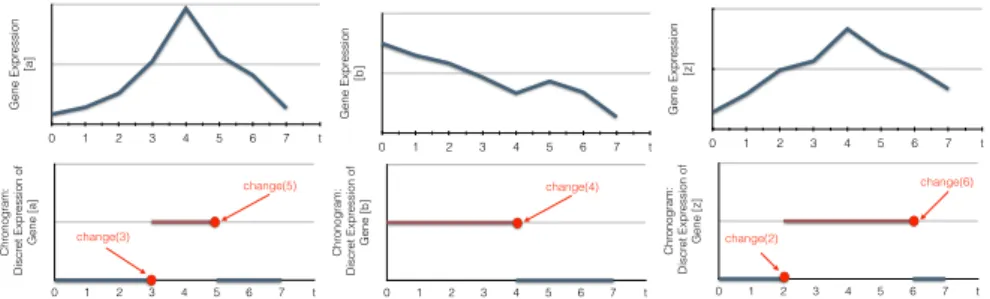
whose chronogram is detailed in Figure 3:
The first change occurs at tmin = t1 = 2, denoted by change(2). It is the
gene z whose value changes from 0 to 1, thus the timed local transition that has
realized this change has this form z0
`
→δ z1, where ` can be any combination of
the values of the regulators at t1− 1 of z.
Let χ ={b → z, a → z, a → a} be the set of regulation influences among the
components of the network. According to χ the set of genes having influence on z
is χz={a, b}. It means that ` = {a?, b?} or ` = {a?} or ` = {b?}. The expression
level of the genes of χzwhen the researched candidate timed local transition (τi)
is ongoing, i.e during the partial steady state between two successive changes (ti
and ti−1). This level is computed from the chronograms as follows:
Algorithm 1MoT-AN: Modeling Timed Automata Networks
INPUT:
- Timed Automata NetworkAN = (Σ, S, T ) with T = ∅;
- a chronogram Γ =S
a∈ΣΓa;
- the regulation influences χ =S
a∈Σχa and
- a maximal in-degree i∈ N∗
OUTPUT: φ a set of Timed Automata Networks that realize the time series
data.
– Let ϕ :=∅
– Step 1: According to the chronogram Γ , for each time step where a
compo-nent a changes its value from ai to aj, with ai, aj∈ S(a):
- Let δ(b) < t be the last time step where b has changed with b∈ χa
- For each l0
∈ ℘(χa),|l0| ≤ i generates all timed local transitions:
τ := (ak, l, al, t− δ) such that δ = δ(b0), b0 ∈ l0, @b00 ∈ l0, δ(b00) > δ(b0) and l = {bi∈ ζ(δ) | b ∈ l0}
- Add all timed local transition τ in ϕ
– Step 2: Generate φ the set of all Timed Automata NetworksAN0 = (Σ,
S, ϕ0)
with ϕ0⊆ ϕ a set of timed local transitions that can realize Γ such that ϕ0
is minimal:
∀AN0= (Σ,S, ϕ0)
∈ φ, 6 ∃ϕ00
⊆ ϕ, ϕ00
Gene Expr ession [a] 0 1 2 3 4 5 6 7 t Gene Expr ession [b] 0 1 2 3 4 5 6 7 t Gene Expr ession [z] 0 1 2 3 4 5 6 7 t Chr onogram: Discr et Expr ession of Gene [a] 0 1 2 3 4 5 6 7 t change(5) change(3) Chr onogram: Discr et Expr ession of Gene [b] 0 1 2 3 4 5 6 7 t change(4) Chr onogram: Discr et Expr ession of Gene [z] 0 1 2 3 4 5 6 7 t change(6) change(2)
Fig. 3. Examples of the discretization of continous time series data into bi-valued chronograms. Abscissa (resp. ordinate) represents time (resp. gene expression levels). In this example, the expression level is discretized according to a threshold fixed to the half of the maximum gene expression value. change(t) indicates that the expression level of a biological component, here a gene, changes its value at a time point t.
- a∈ χz: [a]t= 0∀t ∈ [0, 2] - b∈ χz: [b]t= 1∀t ∈ [0, 2]
Thus `={a0, b1} or `={a0} or `={b1} and the set of candidate timed local
transi-tions is: Tchange(2) = {τ1 = z0
a0 →δ 1 z1, τ2 = z0 b1 →δ 2 z1, τ3 = z0 a0∧b1 −→δ 3 z1}. Since
it is the first change, the delay of each timed local transition is the same:
δ1= δ3= δ3= 2.
The second change occurs at t2= 3 and denoted by change(3). Here it is the
gene a whose state changes from a0 to a1, thus the timed local transition that
realize this change has this form τ = a0
`
→δ a1 where ` can be any combination
of the regulators value at t1 of z. According to χ the genes influencing a are
χa ={a}. It means that ` = {a?} and the expression level of a between t1 and
t2 is a0. So ` ={a0}. Thus there is only one candidate timed local transition:
Tchange(3) ={τ = a0→∅ 1 a1}.
The third change occurs at t3 = 4, change(4). Here it is the gene b whose
value changes from b1 to b0, thus the timed local transition that realize this
change is of this form, τ = b1
`
→δ b0 where ` can be any combination of the
regulators value at t3− 1 of b. According to χ there is no gene that can influence
b, thus no timed local transition can realize this change.
The fourth change occurs at t4= 5, change(5). Here it is a whose expression
decreases and changes from a1 to a0, thus the candidate timed local transition
that could realize this change has this form, τ = a1
`
→δ a0 where ` can be any
combination of the regulators value at t4−1 of a. According to χ the set of genes
having influences on a is χa={a}. Again ` = {a?} and since the expression level
of a since its last change is a1. we have A ={a1} and there is only one candidate
timed local transition:Tchange(5) ={τ = a1
∅
→1 a0}.
The fifth change occurs at t5= 6, change(6). Here it is z whose value changes
the form of: τ = z1 `
→δ z0 where ` can be any combination of the regulators
value at t3− 1 of b. Since χz={a, b}, it means that ` = {a?, b?} or ` = {a?} or
` ={b?} The expression level of a and b at t5− 1 is respectively a0 and b0. Thus
` ={a0, b1} or ` = {a0} or ` = {b0}. The candidate timed local states are:
Tchange(6) ={τ1= z1 a0 →δ 1 z0, τ2= z1 b0 →δ 2 z0, τ3= z1 a0∧b0 −→δ 3 z0}.
The last change of a is at t4= 5 and the last change of b is at t3= 4. Thus
δ1= t5− t4= 1, δ2= t5− t3= 2, δ3= t5− max(t4, t3) = 1.
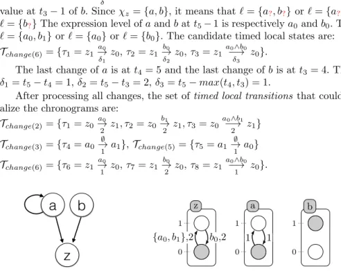
After processing all changes, the set of timed local transitions that could re-alize the chronograms are:
Tchange(2) ={τ1= z0 a0 →2 z1, τ2= z0 b1 →2 z1, τ3= z0 a0∧b1 −→2 z1} Tchange(3) ={τ4= a0 ∅ →1 a1}, Tchange(5)={τ5= a1 ∅ →1 a0} Tchange(6) ={τ6= z1 a0 →1 z0, τ7= z1 b0 →2 z0, τ8= z1 a0∧b0 −→1 z0}.
a
z
b
z 0 1 a 0 1 b 0 1 {a0, b1},2 b0,2 1 1 1Fig. 4. Left: influence graph modeling of the case study example (figure 3). Right, one of the Timed Automata Networks generated by the algorithm 1. The labels of each local transition stands for the local states of the automata which make the transition playable and its delay (time needed for the transition to be performed).
All timed local transitions learned are consistent with all observed time series data and the regulation influences given as input. The used method ensures completeness, we have the full set of timed local transitions that can explain the observations. By generating all minimal subsets of this set of timed local transitions, one of those subset will be the set who realized the observations.
5
Evaluation
In this section, we provide two evaluations of Algorithm 1. We evaluate the
capacity of our algorithm3 to construct models for prediction and the impact of
the quantity of observations on run time. Here we process chronograms obtained from time series data of the DREAM4 challenge [25].
3
All programs, described in this article, for Timed Automata Network generation are implemented in ASP and are available online at: http://www.irccyn.ec-nantes. fr/~benabdal/modeling-biological-regulatory-networks.zip
5.1 DREAM4
In this section, we assess the efficiency of our algorithm through case studies coming from the DREAM4 challenge. DREAM challenges are annual reverse engineering challenges that provide biological case studies. In this section, we focus on the datasets coming from DREAM4. It provides data for systems of different size (10 genes on one hand, 100 genes on the other hand), allowing us to assess the scalability of our approach. The input data that we tackle here consists of the following: 5 different systems each composed of 100 genes, all coming from E. coli and yeast networks. For every such system, the available data are the following: (i) 10 time series data with 21 time points and 1000 is the duration of each time series; (ii) steady state for wild type; (iii) steady states after knocking out each gene; (iv) steady states after knocking down each gene (i.e. forcing its transcription rate at 50%); (v) steady states after some random multifactorial perturbations. We processed all the data. Here, we focus on the management of time series data.
Each time series includes different perturbations that are maintained all time along during the first 10 time points and applied to at most 30% of the genes. In this setting, a perturbation means a significant increase or decrease of the gene expression. In the raw data of the time series, gene expression values are given as real numbers between 0 and 1. To apply our approach, we chose to discretize those data into two to six qualitative values. Increasing the number of qualitatives values from 2 to 4 improves the precision, but then the score decrease from 5, must likely because of overfitting: the relations learned become too precised and can’t be applied on something else than the training data. The best score we obtain were with 4 qualitatives values and are reported in figure 5. Each gene is discretized in an independent manner, with respect to the following procedure: we compute the average value of the gene expression among all data of a time series, then the values between the average and the maximal/minimal value are divided into as many levels. Discretizing the data according to the average value of expression is expected to reduce the impact of perturbation on the discretization and thus on the model learned.
The DREAM4 challenge offers two different problems, which consist in pre-dicting (i) the structure of the gene interactions (in terms of an unsigned directed graph); (ii) attractors in some given conditions. Our method is not designed to tackle the first issue, indeed we need to know those influences. But the models we learn can be applied to predict trajectories and thus attractors. Here we use the influences graphs expected in the first problem as background knowledge (given in appendix) to tackle the attractor prediction part of the challenge.
5.2 Results
For this evaluation, we are given an initial state and 5 different dual gene knock-outs conditions. The goal is to predict the attractor in which the system will fall from the initial state for each dual knockout. Here, we just choose the first model that our algorithm output and use the biggest set of fireable timed local transition at each time step to produce a trajectory until a cycle is detected. The
Benchmark Number of genes MSE insilico size10 1 10 0.086 insilico size10 2 10 0.080 insilico size10 3 10 0.076 insilico size10 4 10 0.039 insilico size10 5 10 0.076
Benchmark Number of genes MSE
insilico size100 1 100 0.052
insilico size100 2 100 0.042
insilico size100 3 100 0.033
insilico size100 4 100 0.033
insilico size100 5 100 0.052
Fig. 5. Evaluation of our method on learning and prediction of the evolution of gene regulatory network benchmarks from the DREAM4 challenge through the Mean Square Error (MSE): 10 variables benchmarks (left) and 100 variables benchmarks (right).
first state of this cycle is reverse discretized and proposed as the predicted state. In the challenge, the quality of the prediction is evaluated by computing the mean square error (MSE) between the predicted state and the expected one. As shown in figure 5, the precision we achieved in those experiments is quite good considering the results of the competitors of the DREAM4 challenge [1]. Their results range between 0.010 and 0.075 for the same evaluation settings, which we are comparable to (0.033 to 0.086) giving us encouraging results. Regarding run time, learning and predicting the trajectories of the benchmarks of 10 genes took less than 30 seconds and the same experiements for the benchmarks of 100 genes took about 3 hours and 20 minutes on one processor Intel Core2 Duo (P8400, 2.26GHz).
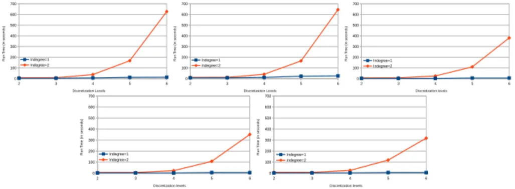
To achieve this score, we had to perform several tests by varying the dis-cretization precision and the complexity of the dynamics learned. Those tests also allows us to assess the scalability of our approach in practice. Figure 6 shows the impact of both timed local transition indegree and discretization level on run time. 2 3 4 5 6 0 100 200 300 400 500 600 700 Indegree=1 Indegree=2 Discretization Levels R u n T im e ( in s e co n d s) 2 3 4 5 6 0 100 200 300 400 500 600 700 Indegree=1 Indegree=2 Discretization Levels R u n T im e ( in s e co n d s) 2 3 4 5 6 0 100 200 300 400 500 600 700 Indegree=1 Indegree=2 Discretization levels R u n T im e ( in s e co n d s) 2 3 4 5 6 0 100 200 300 400 500 600 700 Indegree=1 Indegree=2 Discretization levels R u n T im e ( in s e co n d s) 2 3 4 5 6 0 100 200 300 400 500 600 700 Indegree=1 Indegree=2 Discretization levels R u n T im e ( in s e co n d s)
Fig. 6. Evolution of run time on processing different models inferred from time series data of DREAM4 (100 variables benchmarks), varying indregree of local timed tran-sitions and discretization levels. These tests were performed on a processor Intel Core i7 (4700, 3GHz) with 16GB of RAM.
In the results obtained from the experimentation of our algorithm on the time series data of the DREAM4 we can see the exponential influence on the
run time of the indegree per local transition considered as well as the level of discretization chosen for all the 5 different networks. But it also shows that in practice our approach can tackle big network, here 100 genes.
5.3 Discussion
We propose a new method MoT-AN (algorithm 1) to automatically infer models that could explain the dynamic evolution of the biological system. We illus-trated the merits of this method by applying it on a large real biological system (DREAM4 challenge). As a result we obtain in few seconds models that are proved to be relevant (this relevance is qualified in terms of mean square error with gold standard network) This algorithm is implemented using Answer Set Programming [5,4], thus provides the exhaustive enumeration of all models. The main limit of the approach presented in this paper is the fact that topology of the network is considered as granted. As discussed in the introduction of the paper, there is a wide range of algorithms designed to address this issue. Fur-thermore, such interaction graphs could be deduced from the available reliable databases of biological networks. Some examples of data bases for human reg-ulatory knowledge are: Pathways Interaction Database [20], Human Integrated Pathway DB [32] and Causal Biological Network Database [30].
Various inference approaches [11,20,26] from time series data based on prior knowledge about component interactions have been proposed. But they share a common limit: they focus on static characterization of the interactions and they do not allow to infer dynamic behaviors where delays are involved. The merits of our contribution lie in the fact that we overcome such limits, and we infer delays in a qualitative dynamic modeling of the network.
6
Conclusion and perspectives
In this paper, we propose an approach takes a background knowledge under the form of regulation graph and time series data as an input. The contribution of our method lies in the fact that it identifies the set of interactions between biological components by (1) concertizing the signs (negative or positive) (2) providing thresholds and associating the quantitative time delays. As a result, we have a set of Timed Automata networks that explain the biological network evolution. The algorithm 1 is implemented in ASP. We illustrated the applica-bility and limits of the proposed method through benchmarks from DREAM4. This opens the way to promising applications in the cooperation between biolo-gists and computer scientists. Further works now consist in discussing the kind of information one can get on Timed Automata Network by analyzing the asso-ciated untimed model. We also plan to improve our implementation to make it robust against noisy and scarse data as like in the DREAM8: Heritage-DREAM breast cancer network inference challenge.
References
1. Emna Ben Abdallah, Maxime Folschette, Olivier Roux, and Morgan Magnin. Ex-haustive analysis of dynamical properties of biological regulatory networks with answer set programming. In IEEE International Conference on Bioinformatics and Biomedicine (BIBM), pages 281–285. IEEE, 2015.
2. Jamil Ahmad, Gilles Bernot, Jean-Paul Comet, Didier Lime, and Olivier Roux. Hybrid modelling and dynamical analysis of gene regulatory networks with delays. ComPlexUs, 3(4):231–251, 2006.
3. Tatsuya Akutsu, Takeyuki Tamura, and Katsuhisa Horimoto. Completing networks using observed data. In Algorithmic Learning Theory, pages 126–140. Springer, 2009.
4. Saadat Anwar, Chitta Baral, and Katsumi Inoue. Encoding higher level extensions of petri nets in answer set programming. In Logic Programming and Nonmonotonic Reasoning, pages 116–121. Springer, 2013.
5. Chitta Baral. Knowledge representation, reasoning and declarative problem solving. Cambridge university press, 2003.
6. Werner Callebaut. Scientific perspectivism: a philosopher of sciences response to the challenge of big data biology. Studies in History and Philosophy of Science Part C: Studies in History and Philosophy of Biological and Biomedical Sciences, 43(1):69–80, 2012.
7. Jean-Paul Comet, Jonathan Fromentin, Gilles Bernot, and Olivier Roux. A formal model for gene regulatory networks with time delays. In Computational Systems-Biology and Bioinformatics, pages 1–13. Springer, 2010.
8. Jianqing Fan, Fang Han, and Han Liu. Challenges of big data analysis. National science review, 1(2):293–314, 2014.
9. Maxime Folschette, Lo¨ıc Paulev´e, Katsumi Inoue, Morgan Magnin, and Olivier Roux. Identification of Biological Regulatory Networks from Process Hitting mod-els. Theoretical Computer Science, 568(0):49 – 71, 2015.
10. Paul Freedman. Time, petri nets, and robotics. Robotics and Automation, IEEE Transactions on, 7(4):417–433, 1991.
11. Emmanuelle Gallet, Matthieu Manceny, Pascale Le Gall, and Paolo Ballarini. An ltl model checking approach for biological parameter inference. In International Conference on Formal Engineering Methods, pages 155–170. Springer, 2014. 12. Yaron AB Goldstein and Alexander Bockmayr. A lattice-theoretic framework for
metabolic pathway analysis. In Computational Methods in Systems Biology, pages 178–191. Springer, 2013.
13. Inman Harvey and Terry Bossomaier. Time out of joint: Attractors in asynchronous random boolean networks. In Proceedings of the Fourth European Conference on Artificial Life, pages 67–75. MIT Press, Cambridge, 1997.
14. Sun Yong Kim, Seiya Imoto, and Satoru Miyano. Inferring gene networks from time series microarray data using dynamic bayesian networks. Briefings in bioin-formatics, 4(3):228–235, 2003.
15. Chushin Koh, Fang-Xiang Wu, Gopalan Selvaraj, and Anthony J Kusalik. Using a state-space model and location analysis to infer time-delayed regulatory networks. EURASIP Journal on Bioinformatics and Systems Biology, 2009(1):1, 2009. 16. Ali Sinan Koksal, Yewen Pu, Saurabh Srivastava, Rastislav Bodik, Jasmin Fisher,
and Nir Piterman. Synthesis of biological models from mutation experiments. In ACM SIGPLAN Notices, volume 48, pages 469–482. ACM, 2013.
17. Tie-Fei Liu, Wing-Kin Sung, and Ankush Mittal. Learning multi-time delay gene network using bayesian network framework. In Tools with Artificial Intelligence, 2004. ICTAI 2004. 16th IEEE International Conference on, pages 640–645. IEEE, 2004.
18. Vivien Marx. Biology: The big challenges of big data. Nature, 498(7453):255–260, 2013.
19. Hiroshi Matsuno, Atsushi Doi, Masao Nagasaki, and Satoru Miyano. Hybrid petri net representation of gene regulatory network. In Pacific Symposium on Biocom-puting, volume 5, page 87. World Scientific Press Singapore, 2000.
20. Max Ostrowski, Lo¨ıc Paulev´e, Torsten Schaub, Anne Siegel, and Carito Guzi-olowski. Boolean network identification from multiplex time series data. In Inter-national Conference on Computational Methods in Systems Biology, pages 170–181. Springer, 2015.
21. Nicola Paoletti, Boyan Yordanov, Youssef Hamadi, Christoph M Wintersteiger, and Hillel Kugler. Analyzing and synthesizing genomic logic functions. In Computer Aided Verification, pages 343–357. Springer, 2014.
22. Lo¨ıc Paulev´e. GoalOriented Reduction of Automata Networks. In CMSB 2016 -14th conference on Computational Methods for Systems Biology, 2016. accepted. 23. Lo¨ıc Paulev´e, Courtney Chancellor, Maxime Folschette, Morgan Magnin, and
Olivier Roux. Logical Modeling of Biological Systems, chapter Analyzing Large Network Dynamics with Process Hitting, pages 125 – 166. Wiley, 2014.
24. Lo¨ıc Paulev´e, Morgan Magnin, and Olivier Roux. Refining dynamics of gene regu-latory networks in a stochastic π-calculus framework. In Transactions on Compu-tational Systems Biology XIII, volume 6575 of Lecture Notes in Comp Sci, pages 171–191. Springer, 2011.
25. Robert J Prill, Julio Saez-Rodriguez, Leonidas G Alexopoulos, Peter K Sorger, and Gustavo Stolovitzky. Crowdsourcing network inference: the dream predictive signaling network challenge. Science signaling, 4(189):mr7, 2011.
26. Julio Saez-Rodriguez, Leonidas G Alexopoulos, Jonathan Epperlein, Regina Sam-aga, Douglas A Lauffenburger, Steffen Klamt, and Peter K Sorger. Discrete logic modelling as a means to link protein signalling networks with functional analysis of mammalian signal transduction. Molecular systems biology, 5(1):331, 2009. 27. Thomas Schaffter, Daniel Marbach, and Dario Floreano. Genenetweaver: in silico
benchmark generation and performance profiling of network inference methods. Bioinformatics, 27(16):2263–2270, 2011.
28. Heike Siebert and Alexander Bockmayr. Temporal constraints in the logical anal-ysis of regulatory networks. Theoretical Computer Science, 391(3):258–275, 2008. 29. Chao Sima, Jianping Hua, and Sungwon Jung. Inference of gene regulatory
net-works using time-series data: a survey. Current genomics, 10(6):416–429, 2009. 30. Marja Talikka, Stephanie Boue, and Walter K Schlage. Causal biological network
database: A comprehensive platform of causal biological network models focused on the pulmonary and vascular systems. Computational Systems Toxicology, pages 65–93, 2015.
31. Ren´e Thomas. Regulatory networks seen as asynchronous automata: a logical description. Journal of theoretical biology, 153(1):1–23, 1991.
32. Namhee Yu, Jihae Seo, Kyoohyoung Rho, Yeongjun Jang, Jinah Park, Wan Kyu Kim, and Sanghyuk Lee. hipathdb: a human-integrated pathway database with facile visualization. Nucleic acids research, 40(D1):D797–D802, 2012.
33. Zhi-Yong Zhang, Katsuhisa Horimoto, and Zengrong Liu. Time series segmentation for gene regulatory process with time-window-extension. 2008.
34. Wentao Zhao, Erchin Serpedin, and Edward R Dougherty. Inferring gene regulatory networks from time series data using the minimum description length principle. Bioinformatics, 22(17):2129–2135, 2006.
A
Appendixes
A.1 Proof of Theorem 1
Theorem 3 (Completeness). Let AN = (Σ, S, T ) be a Timed Automata
Network, Γ be a chronogram of the components of AN , i ∈ N and R ∈ T
be the set of timed local transitions that realized the chronogram Γ such that
(ai, l, aj, δ) ∈ R =⇒ |l| ≤ i. Let χ be the regulation influences of all a ∈ Σ.
Let AN0 = (Σ,S, ∅) be a Timed Automata Network. Given AN0,Γ , χ and i as
input, Algorithm 1 is complete: it will output a set of Timed Automata Network
φ, such that ∃AN00= (Σ,S, ϕ0)
∈ φ with R ⊆ ϕ0.
Proof. Let us suppose that the algorithm is not complete, then there is a timed
local transitionh∈ R that realized Γ and h 6∈ ϕ0. In Algorithm 1, after step1, ϕ
contains all timed local transitions that can realize each change of the chronogram
Γ . Here there is no timed local transition h ∈ R that realizes Γ which is not
generated by the algorithm, soh∈ ϕ. Then it implies that at step 2, ∀ϕ0, h
6∈ ϕ0.
But sinceh realizes one of the change of Γ and h is generated at step 1, then it
will be present in one of the minimal subset of timed local transitions. Such that
h will be in one of the networks outputted by the algorithm.ut
A.2 Proof of Theorem 2
Theorem 4 (Complexity). Let AN = (Σ, S, T ) be a Timed Automata
Net-work, |Σ| be the number of automaton of AN and η be the total number of
local state of a automaton of AN . Let Γ be a chronogram of the components
of AN over τ units of time, such that c is the number of changes of Γ . The
memory use of Algorithm 1 belongs toO(τ· i|Σ|+1· 2τ ·i|Σ|+1) that is bounded by
O(τ · |Σ|T ·|Σ||Σ|+1). The complexity of learning
AN by generating timed local
transitions from the observations ofΓ with Algorithm 1 belongs to O(c· i|Σ|+1+
22·τ ·i|Σ|+1
+c·2τ ·i|Σ|+1), that is bounded by O(τ
· 23·τ ·|Σ||Σ|+1 ).
Proof. Let i be the maximal indegree of a timed local transition in AN , 0 ≤
i ≤ |Σ|. Let p be an automaton local state of AN then |Σ| is maximal the
number of automaton that can influence p. There is i|Σ| possible combinations
of those regulators that can influences p at the same time forming a timed local
transition. There is at mostτ possible delays, so that there are τ·|Σ|·i|Σ|possibles
timed local transitions, thus in Algorithm 1 at step 1, the memory is bounded by O(τ· i|Σ|+1), which belongs to O(τ
· |Σ||Σ|+1) since 0
≤ i ≤ |Σ|. Generating all
minimal subsets of timed local transitionsϕ ofAN that can realize Γ can require
to generate at most 2τ ·|Σ|·i|Σ|+1 set of rules. Thus, the memory of our algorithm
belongs toO(τ· i|Σ|+1
· 2τ ·i|Σ|+1
) and is bounded by O(τ· |Σ||Σ|+1
· 2τ ·|Σ||Σ|+1 ).
The complexity of this algorithm belongs toO(c· i|Σ| + 1). Since 0 ≤ i ≤ |Σ|
and0≤ c ≤ τ the complexity of Algorithm 1 is bounded by O(τ · |Σ||Σ|+1)).
Generating all minimal subsets of timed local transitionsϕ ofAN0that realize
has to be compared with the others to keep only the minimal ones, which costs O(22·τ ·i|Σ|+1
). Furthermore, each set of timed local transitions has to realize each
change of Γ , it requires to check c changes and it costs O(c· 2τ ·i|Σ|+1). Finally,
the total complexity of learning AN by generating timed local transitions from
the observations of Γ belongs to O(c· i|Σ|+1+ 22·τ ·i|Σ|+1
+ c· 2τ ·i|Σ|+1). that is
bounded by O(3τ· 22·τ ·|Σ||Σ|+1
). ut
A.3 DREAM4: Influence network
The figure 7 presents the regulatory graph that we are based on to identify the signs (negative or positive), the thresholds and the quantitative time delays of the learned transitions.
Fig. 7. The influence network of the DREAM4 challenge model (100 genes) given by GeneNetWeaver (GNW) data generator [27]. Each node is a gene and each edge is an influence from the source to the target gene.
![Fig. 7. The influence network of the DREAM4 challenge model (100 genes) given by GeneNetWeaver (GNW) data generator [27]](https://thumb-eu.123doks.com/thumbv2/123doknet/8236644.277044/21.892.307.612.430.728/influence-network-dream-challenge-model-genes-genenetweaver-generator.webp)
