Is Balanced Harvest a good idea? An ecosystem modelling approach to rebuild fisheries and trophic structure of the Celtic Sea

HAL Id: dumas-02619170

https://dumas.ccsd.cnrs.fr/dumas-02619170

Submitted on 25 May 2020

HAL is a multi-disciplinary open access archive for the deposit and dissemination of sci-entific research documents, whether they are pub-lished or not. The documents may come from teaching and research institutions in France or abroad, or from public or private research centers.

L’archive ouverte pluridisciplinaire HAL, est destinée au dépôt et à la diffusion de documents scientifiques de niveau recherche, publiés ou non, émanant des établissements d’enseignement et de recherche français ou étrangers, des laboratoires publics ou privés.

Is Balanced Harvest a good idea? An ecosystem

modelling approach to rebuild fisheries and trophic

structure of the Celtic Sea

Ilan Perez

To cite this version:

Ilan Perez. Is Balanced Harvest a good idea? An ecosystem modelling approach to rebuild fisheries and trophic structure of the Celtic Sea. Life Sciences [q-bio]. 2019. �dumas-02619170�

Is Balanced Harvest a good idea?

An ecosystem modelling approach to rebuild fisheries and

trophic structure of the Celtic Sea

Par : Ilan PEREZ

Soutenu à Rennes le 10 septembre 2019

Devant le jury composé de :

Président et enseignant référent : Olivier LE PAPE Maître de stage : Didier GASCUEL

Autres membres du jury (Nom, Qualité) Marianne ROBERT, chercheuse à Ifremer STH Lorient Morgane TRAVERS-TROLET, chercheuse à Ifremer Nantes EMH

Les analyses et les conclusions de ce travail d'étudiant n'engagent que la responsabilité de son auteur et non celle d’AGROCAMPUS OUEST Ce document est soumis aux conditions d’utilisation

«Paternité-Pas d'Utilisation Commerciale-Pas de Modification 4.0 France» disponible en ligne http://creativecommons.org/licenses/by-nc-nd/4.0/deed.fr

AGROCAMPUS OUEST CFR Angers CFR Rennes Année universitaire : 2018-2019 Spécialité : SML- Biologie

Spécialisation (et option éventuelle) : Sciences Halieutiques et Aquacoles (Ressources et Ecosystèmes Aquatiques)

Mémoire de fin d’études

d’Ingénieur de l’Institut Supérieur des Sciences agronomiques, agroalimentaires, horticoles et du paysage

de Master de l’Institut Supérieur des Sciences agronomiques, agroalimentaires, horticoles et du paysage

Table of content

Remerciements Acknowledgements ... 7

Tables and figures... 10

Abbreviations ... 11

1. Introduction ... 1

1.1. The long History of human impact on marine resources ... 1

1.2. Impacts of fishing on ecosystem structure ... 1

1.3. A science-based management of fisheries? ... 2

1.4. Ecosystem approach to fisheries and the Balanced Harvest theory ... 3

1.5. Analyzing BH using ecosystem models ... 4

1.6. Scientific objective of the current work ... 5

2. Methods ... 6

2.1. Study site ... 6

2.2. The Ecopath with Ecosim model ... 7

Principles and equations ... 7

Functional group composition ... 8

Fitting Ecosim model ... 9

2.3. Fishing scenarios... 11

2.4. Comparison of scenarios ... 15

3. Results ... 16

3.1. Ecopath flow diagram and Ecosim fitting ... 16

3.2. Locked in time: Maintaining the current fishing strategy. ... 18

3.3. The MSY management scenario ... 20

3.4. Comparison between the FMSY scenario and the restricted BH strategies ... 21

3.5. Incremental BH strategies ... 22

Balanced harvest on target fish species without TAC regulation... 22

Balanced Harvest on bycatch fish species, targeted cephalopods and crustaceans ... 23

Full Balanced Harvest ... 23

3.6. Ecological indicators ... 26

4. Discussion ... 27

4.1. Limits of the methods ... 27

4.2. Status quo: still a lot to do for sustainable fisheries ... 29

4.4. Balancing the harvest of main caught species, the solution? ... 31

4.5. Toward full balanced harvest: successes and failures... 32

4.6. Future work and suggestions for improvement ... 34

5. Conclusion ... 35

References ... 36

Supplementary list



Supplementary I – Ecopath with Ecosim outputs and fit

42

Remerciements Acknowledgements

À l'issue de ces 6 mois de stages intensifs, je souhaite remercier vivement le pôle halieutique d'Agrocampus Ouest pour son accueil d'un étudiant qui n'est monté que d'un étage.

Merci à toute l'équipe Cath, Mathilde, Olivier, Hervé, Pierre, Léa, Auriane, Elodie, Hubert, Marie, Thom, Max, Marine, Etienne, Jérôme, Catherine, Noémie Alicia et JB pour votre bonne humeur et vos bons conseils.

Un mot en particulier à Julie, Lucile et bien sûr Christelle, pour votre soutien indéfectible lors des coups durs et des baisses de moral. Christelle, on a fait une bonne équipe de stagiaires en galère, merci d'être toi, toujours le smile et des discussions passionnantes et si apaisantes dans lors de notre siège au bureau pour l'écriture du rapport.

Merci à Pierre-Yves, avec qui les interactions ont été riches et passionnantes, à Lorient comme à l'AFH. Bon courage pour l'écriture de cette thèse et je t'attends de pied ferme pour l'écriture du papier !

Merci à ma super coloc’ Linda, qui s’est démenée pour rendre notre appart Feng Shui pour canaliser nos énergies négatives éveillées par le stress du stage (arrête de mettre mes couteaux au lave-vaisselle je t’en supplie).

Merci énormément Laura et à mes amis oceano de longue date, la perche Suédoise, la mouffette Tasmanienne et le passe partout des marine mammals, qui m'ont soutenu plus que jamais dans ma fastidieuse et vaine recherche d'emploi et d'avenir en thèse. Vos mots sont toujours forts de sens et vous avez su me faire relever la tête.

My last words will be for Jennifer and Didier, of course. Two supervisors with sometimes very divergent points of view, who both trusted me for these last 6 months. Didier, thank you for your availability even if you are the person with the worst schedule I have never seen before. You have this power to make people motivated again, even after two hours of brainstorming (maybe more brainmelting). I am proud to have worked with you and I am looking forward to collaborate for the next 2 months.

Jenni, more than a supervisor, you were a supporting friend. We worked side by side, and we shared more than science in our discussions during lab's park meetings. Doubts, fears, phylosophy of life, bullshit...that was refreshing.

Now, French because if I speak in English while not talking about Science you will yell at me again. Je te promets que je n’oublierais plus les « the » et le « would like » !

Tables and figures

Number

Caption

Fig. 1 Comparison of common exploitation rate on trophic levels and production rate

Fig. 2 Idealized community size spectrum of unexploited community and balanced harvest community Fig. 3 Map of the Celtic Sea ICES areas VII.e-j and the model area

Fig. 4 Composition of annual landings from Celtic Sea fisheries from 1950 to 2016 Fig. 5 Flow diagram of the Ecopath model

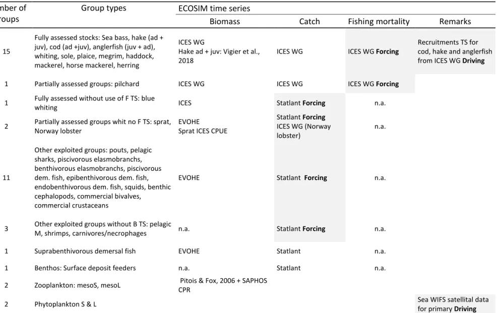
Fig. 6 Fishing mortality of functional groups in 2016

Fig. 7 Trophic spectrums of biomass and catch for Sc0, Status quo and current state Fig. 8 Changes in biomass of functional groups in the Status quo scenario

Fig. 9 Effects of FMSY scenario on biomass of unfished system

Fig. 10 Trophic spectrums of biomass impact and catch for Status and FMSY scenarios Fig. 11 Trophic spectrums of F, B and Yratio of BH TAC strategies

Fig. 12 Trophic spectrums of F, B and Yratio of incremental BH strategies Fig. 13 Zoom of Fig. 12 on TL 3.5-5

Fig. 14 Ecological indicators comparison

Tab. 1 Times series used in fitting the Ecosim model

Abbreviations

Abbrev.

Description

BH

Balanced Harvest

CBD

Convention on Biological Divesity

EAF

Ecosystem Approach to Fisheries

EUMOFA

European market observatory for fisheries and aquaculture

products

EVOHE

EValuation des ressources Halieutiques de l'Ouest de l'Europe

EwE

Ecopath with Ecosim

FAO

Food and Agriculture Organization of the United Nations

ICES

International Council for Exploration of the Sea

IUCN

International Union for Conservation of Nature

MSY

Maximum Sustainable Yield

Sc

Scenario

TAC

Total Allowable Catch

UN

United Nations

1

1. Introduction

1.1. The long History of human impact on marine resources

The history of human impacts on aquatic ecosystems spreads across the millennia and is almost as ancient as humankind itself. Marine fauna has played an important role for the development of coastal tribes, supplying food and materials for housing, tools and clothing. Then fish, bivalves, whales and seals began to be target of ancestral fisheries, leading to the rarefaction of some of the few stocks that were accessible with primitive gears. In the European Middle Age, professional fishing and seafood consumption was confined to the coastal zone due to fear of great seas, and not adapted sailboats and conservation means (Mollat, 1987; Sarhage and Lundbeck, 2012). While some documents reported changes in yields and length of exploited fish such as the herring in North Sea in the 13th _{century (Gascuel, 2019). The common thinking still} considered marine resources as unlimited at that time, and until the end of the 19th _{century. With} 1850 came the exponential growth of human population. In 160 years, global population increased by 600% (United Nations, 2017). Global demand of animal protein from seafood inflated in parallel with population gain, multiplied by three during the 20th _{century, reaching 20.2 kg/capita/year} nowadays (FAO, 2018). To supply this demand, industrialization occurred to modernize fisheries, with the emergence of trawlers with steam and then combustion engine, allowing catching fish faster, further and every time (Gascuel, 2019). Within the 1,200 fish species known in European waters (IUCN, 2014), fisheries mainly selected icon species such as cod, herring, hake, sole, plaice, pilchard, halibut, herring and mackerel. However, over the last decades, the diversity of catch increased from 8 to 24 exploited species on average and overexploitation expanded affecting progressively numerous stocks such as large demersal fish, that have been historically dominant in the catch (Gascuel et al., 2016).

1.2. Impacts of fishing on ecosystem structure

European fisheries affect unevenly the ecosystems. In fact, they were built on highly selective practices, due to cultural and economic preferences: “value is more important than volume” (Kolding and Zwieten, 2011; Kolding et al., 2016). Thus, fishing impacts the top of the trophic pyramid by applying a higher fishing mortality on highly valuable predator species that are less productive (Costello et al., 2012) (Fig. 1). The effects of selective fishing on fish populations and communities have been well studied and documented since the 1990’s. Changes in species

2 abundance and size distributions due to predators overfishing disturbed the trophodynamic of European marine ecosystems, fostering small species with a shorter life cycle (Pauly et al., 1998; Borrel, 2013). Predators play a key role in marine ecosystems, by top-down controlling their prey abundance. They are also considered as architects of biodiversity, because of the pressure they exert on other species. The loss of predators thus deeply disturbs functional diversity and the stability of marine ecosystems, making them less resistant and less resilient to environmental and anthropogenic pressures (Garcia et al., 2003; Isbell et al., 2015).

1.3. A science-based management of fisheries?

Since the 1980’s, scientific advices have been more considered in European fisheries management, which is especially advised by the International Council for Exploration of the Sea (ICES). The 1982 United Nations Convention on the Law of the Sea and the EU Regulation 1380/2013, adopted the concept of Maximum Sustainable Yield (MSY) as the cornerstone and the primary goal of fisheries management (Mace, 2001; Zhang et al., 2016). Today, ICES provides assessments for 397 stocks but FMSY values are provided for 23% of them and 12% have a biomass above the level that can produce MSY (Froese et al., 2016a). The status quo is still far from leading to a sustainable state, 64% of these stocks still being overexploited (ibidem), therefore policies are moving forward to reach the MSY harvesting goal. However, the MSY

Fig. 1: Comparison of common exploitation rates (green line) and production rates (black line)

across trophic levels.

3 approach has long been criticized for (i) being estimated using single-species models, (ii) aiming to maximize and sustain catch of target species without any consideration of the whole ecosystem health (Pauly et al, 2002; Hilborn, 2007; Zhang et al., 2016).

1.4. Ecosystem approach to fisheries and the Balanced Harvest theory

The concept of the Ecosystem Approach to Fisheries (EAF) has been proposed as a holistic framework for a sustainable utilization of aquatic production while preserving functioning of the ecosystem (CBD, 1992; FAO, 2003; Garcia et al., 2003; Kolding et al., 2016). It especially aims at maintaining the structure and functioning of aquatic communities, assuming it would allow the ecosystem to continue providing all ecosystem services that are crucial for humans and other species welfare (Garcia et al., 2015).

In this framework, balanced harvest (BH) has been suggested as a new paradigm of fisheries management in order to meet the objectives of the EAF, ensuring high and sustainable yields while rebuilding and maintaining ecosystem structure and functioning (Zhou et al., 2010; Garcia et al., 2012). The idea of a balanced multispecies harvest was born in the 1950’s and has been formally theorized and proposed in 2010 by the Fisheries Expert Group of the IUCN Commission on Ecosystem Management (Garcia et al., 2011). BH was formerly defined as “a fishery management strategy distributing a moderate fishing pressure across the widest possible range of species, stocks, and sizes of animals within an ecosystem, in proportion to their natural productivity so that the relative size and species composition is maintained’’ (Garcia et al., 2012). Zhou et al. (2019) elaborated this definition and described BH as the “management strategy and collective fishing activities that impose moderate fishing mortality on each utilisable ecological group in proportion to its production, to support long-term total sustainable yields while minimizing fishing impact on the relative species, size, and sex composition within an ecosystem”. In other words, BH can be considered as an alternative alternative fishing strategy where all organisms from zooplankton to top-predators are harvested, which moves fisheries management toward an ecosystem approach (Fig.2). This concept generated lots of questions and debates about its goals, its feasibility and its real efficiency (e.g. Froese et al. 2016b; Pauly et al. 2016). A main argument in favor of BH is that applying such fishing strategy would produce higher total catches while rebuilding the biomass of predators (Garcia et al., 2011, 2015, 2016; Kolding et al., 2016; Reid et al., 2016). But BH has been also criticized by a few scientists arguing that exploitation of all trophic levels may lead to a large ecosystem impact, due to the cumulative effects of fishing along the food web. In contrast, BH is also criticized for its many implications, in relation to

4 selectivity, protection of juveniles, and protected species as well as technological and market constraints that are often conflicting. Finally, BH is also suspected to encourage the development of industrial fisheries exploiting low trophic levels, at the expense of European artisanal fisheries targeting higher and more valuable trophic levels.

1.5. Analyzing BH using ecosystem models

Because there is no explicit implementation of BH in any ecosystem, ecosystem modelling is the only solution to assess the effects of a BH implementation on ecosystem structure and functioning. The consequences of BH on ecosystems at species or size scale have been evaluated with various models in numerous studies (Zhou et al. 2019). Most of them used Size-spectrum models (e.g. Froese et al. 2016b ; Reid et al. 2016), but there are a few ecosystem model such as Atlantis models (Garcia et al., 2012; Nilsen, 2018) and Ecopath with Ecosim models (Garcia et al., 2012, Kolding et al., 2016a) available. These approaches emphasized the difficulty in modelling balanced harvest across, species and sizes and functional groups; emerging from

Fig.2: An idealized community size spectrum of unexploited community (solid red) and balance

5 how productivity is specified at individual size or population level. Zhou et al. (2019) states that applying a fishing mortality rate (F) solely based on average productivity (P/B) of each size or functional group could lead to depletion of species with low production, against the goals of BH, which would not be the case if F was based on Production (P). (Zhou et al. 2019). This statement still has to be tested. Moreover, P/B is readily available from stock assessment data (i.e. total mortality with steady state assumptions), while P requires accurate knowledge on biomass. Previous studies found controversial results about effects of BH on ecosystem biomass, structure and functioning. But these studies were mainly focused on maximization and sustainability of total catches (Ibidem). Heath et al. (2017) explored BH implementations by leading a conceptual approach in the context of Scottish waters, taking into consideration feasibility and the social acceptation of BH toward. Research on BH is in its early stages and descriptive contextual studies with EwE are rare. Despite critics and debates about BH, additional research must be conducted to assess the effects and feasibility of implementing a balanced harvest approach in the real world.

1.6. Scientific objective of the current work

In this study, I tested the Balanced Harvest strategy on the Celtic Sea, using the Ecopath with Ecosim approach (Christensen & Walters, 2005). Like most of the Western world fisheries Celtic sea is a well-studied ecosystem and a new EwE model has been recently built by Hernvann et al. (in prep.). Like most of Western world fisheries, Celtic sea stocks have been over exploited and fishing mortalities now tend to reach FMSY for species under Total Allowable Catch (TAC) regulation. Thus the scientific question of this work is: can we test the feasibility of implementing a BH strategy and can we assess its effects on biomass and catch, using an EwE model such as the one developed in the Celtic sea? More especially, the following study aims to (i) investigate if BH restricted to species under TAC regulation would lead to more sustainable, balanced and productive fisheries than if they were harvested at FMSY and (ii) assess the effects on ecosystem structure and functioning of incremental BH scenarios, from the current range of exploited species toward full BH.

6

2. Methods

2.1. Study site

The Ecopath with Ecosim (EwE) trophic model of the Celtic sea matches the ICES division VIIe-j; and is delimited by the coast of UK, Ireland and France to the 200 m isobaths, it covers an area of 246,000 km² (Fig.3). Although part of its delimitation is administrative, its unique hydrological features distinguish the Celtic sea from the bordering areas: the Eastern Channel, the Bay of Biscay and the Irish Sea. The commercial fisheries occurring in these waters target a large number of stocks, and catches have increased from 320,000 t in 1980 to 350,000 t in 2017 in areas VII.e-j, (Mateo et al., 2017; Moullec et al., 2017). In the Celtic Seas Ecoregion

(ICES areas

VI.a-b, VIIa-j)

, fisheries are mainly pelagic, using mid-water trawling, mostly catching blue whiting, mackerel, herring and horse mackerel. Demersal fisheries target hake and anglerfish, which are high valuable species (Fig. 4).

Fig.3: Map of the Celtic Sea ICES areas VII.e-j and the model area (hatched).

Pers. Comm. Pierre-Yves Hernvann.

7

2.2. The Ecopath with Ecosim model

Principles and equations

Ecopath is a mass-balance model that represents the trophic structure and functioning of aquatic ecosystems (Christensen and Pauly, 1992; Christensen and Walters, 2004; Polovina, 1984). In this widely used approach (Colleter, et al., 2015), the ecosystem is modelled using functional boxes, in which all species are similar in size, food preferences, predators, habitat and life cycle. The master equations describe (i) the production of each functional group and (ii) the energy balance:

𝐵

_𝑖

× (

𝑃 𝐵

)

_𝑖

= ∑

𝐵

𝑗 𝑁 𝑗=1

× (

𝑄 𝐵

)

_𝑗

× 𝐷𝐶

𝑗𝑖

+ (

𝑃 𝐵

)

_𝑖

× 𝐵

𝑖

× (1 − 𝐸𝐸

𝑖

) + 𝑌

𝑖

+ 𝐸

𝑖

+ 𝐵𝐴

𝑖

𝑄

_𝑖

= 𝑃

_𝑖

+ 𝑅

_𝑖

+ 𝑈𝐴

_𝑖

Where

𝐵

_𝑖 is the biomass of the group

𝑖

(t.km-2_),

₍

𝑃

𝐵

)

_𝑖 is the productivity, which is equal to the total mortality

𝑍

(year -1_{) under equilibrium assumption,}

_𝐸𝐸

𝑖 is the ecotrophic efficiency (i.e. the fraction

of total production used in the system),

(

𝑄

𝐵

)

_𝑗 is the consumption rate of the predator

𝑗

on the

Fig.4: Composition of annual landings from the Celtic Seas Ecoregion (area VI.a-b, VIIa-j) fisheries

between 1950 and 2016.

Data from ICES, 2018

Lan d in gs (t h o u san d s o f to n s)

8 group

𝑖

(year -1_),

𝐷𝐶

𝑗𝑖 is the fraction by weight of prey

𝑖

in the average diet of predator

𝑗

,

𝑌

𝑖 is the catch (t.km-2_.year -1_),

𝐸

𝑖 is the net emigration,

𝐵𝐴

𝑖 is the biomass accumulation,

𝑄

𝑖 is the consumption,

𝑃

_𝑖 is the production,

𝑅

_𝑖 is the respiration and

𝑈𝐴

_𝑖 is the unassimilated food caused by excretion and egestion. To balance the model, three of the input parameters

(

𝑃

𝐵

)

_𝑖,

(

𝑄 𝐵

)

_𝑗,

𝐵

𝑖 or

𝐸𝐸

_𝑖, have to be set for each group. Because of the mass balance assumption (equation 2), all

𝐸𝐸

_𝑖 values must be lower or equal to 1.

Ecosim is the temporal dynamic version of Ecopath, allowing users to analyze past trends and to project changes in biomass and biomass flow rates by taking into account modifications in prey-predator relationships and fishing mortality through time (Walters et al., 1997; Pauly et al., 2000; Christensen & Walters, 2005). The biomass growth rate is expressed as:

𝑑𝐵

_𝑖

𝑑𝑡

= 𝑔

𝑖

× ∑

𝑄

𝑗𝑖

− ∑

𝑄

𝑖𝑗 𝑁 𝑗=1

+ 𝐼

_𝑖

− (𝑀0

_𝑖

+ 𝐹

_𝑖

+ 𝑒

_𝑖

) × 𝐵

_𝑖 𝑁 𝑗=1

Where

(𝑑𝐵_𝑖)/𝑑𝑡

represents the growth rate during the time interval

𝑑𝑡

of group

𝑖

in terms of its biomass,

𝑔

_𝑖 is the net growth efficiency,

𝑀0

_𝑖 the non-predation natural mortality rate,

𝑄

_𝑗𝑖 is the consumption of prey

𝑗

by group

𝑖

,

𝑄

_𝑖𝑗 is the consumption of group

𝑖

by predator

𝑗

,

𝐹

_𝑖 is the annual fishing mortality rate, and

𝑒

_𝑖 is the emigration rate. The

𝑄

_𝑗𝑖 parameter, which is determined by predator-prey relationships, is based on the foraging arena theory, in which it is assumed that spatial and temporal restrictions in predator and prey activity cause partitioning of each prey population into vulnerable and invulnerable components (Walters and Kitchell, 2011 ; Ahrens et al., 2012).Then, the transfer rate between these two components for each prey-predator couple (

𝑣

_𝑖𝑗) determines if control is top-down, bottom-up or of an intermediate type (Christensen and Walters, 2005).

Functional group composition

A preexisting Ecopath model of the Celtic Sea was developed by Moullec et al. (2017), built upon a model of the Biscay-Celtic area (Guénette and Gascuel, 2009; Bentorcha et al., 2017), containing 43 functional groups. With the aim of building a tool for supporting the implementation of EAF in this area, most commercially exploited species (both demersal such as anglerfish and

9 pelagic fish such as horse mackerel, supplementary I) were modelled as monospecific groups. Among these groups, hake and cod were split into two stanzas (juv and ad). Hernvann et al. (accepted) recently updated the model by restructuring some groups, leading to a total number of 54 functional groups. Some groups essentially based on taxonomic group or size class were modified to integrate more trophic considerations and anglerfish was split into two stanza based on recent trophic studies (Issac et al., 2017). A significant improvement of the model was the estimation of a new diet matrix using a novel framework (Hernvann et al., accepted, 2018) to integrate recent isotopic and gut content analyses together with literature knowledge mainly used previously for the diet matrix of Moullec et al. (2017)

A 2016 Ecopath model was balanced by Hernvann et al. (in prep.) especially using output of ICES assessment for commercial species, and biomass estimated from EVOHE surveys. Then the 1985 model was derived from it, changing values of catches (Y), biomass (B), productivity (P/B) and dietary proportions based on raw changes in functional groups abundance according to the available abundance data (details of 1985 Ecopath model in Supplementary I)

Fitting Ecosim model

We fitted the Ecosim model to observed time series of abundance, biomass and catch over the period 1985-2016. Based on the foraging arena theory (Ahrens et al., 2012) we adjusted the vulnerabilities using the automatic search of 30 predators and 30 prey-predator couples with the aim to have the lowest sum of squares between the observed biomass and catch values of the time series and the simulated biomass and catch values from the model.

We used fishing mortality time series from ICES Working Groups (hereafter ICES WG) as forcing functions in place of a fishing effort index. When it was unavailable, especially in the case of multispecies groups, time series of catch were used as forcing function. Biomass data from ICES WG was used for the fitting as relative biomass data, since stocks distribution range was frequently out of model borders. For all groups for which no stock assessment was available abundance indices from EVOHE cruises (Mahe and Laffargue, 1987) wereused as relative biomass time-series. (Supplementary II).

For multistanza groups, recruitment data from ICES WG were used as driving time series to improve the quality of the juvenile stanza biomass variation over time.

Finally, for phytoplankton groups, primary production data from remote sensing and biochemistry surveys were used as driving time series.

Number of

groups

Group types

ECOSIM time series

Biomass

Catch

Fishing mortality

Remarks

15

Fully assessed stocks: Sea bass, hake (ad + juv), cod (ad +juv), anglerfish (juv + ad), whiting, sole, plaice, megrim, haddock, mackerel, horse mackerel, herring

ICES WG Hake ad + juv: Vigier et al.,

2018

ICES WG ICES WG Forcing

Recruitments TS for cod, hake and anglerfish from ICES WG Driving

1 Partially assessed groups: pilchard ICES WG ICES WG ICES WG Forcing

1 Fully assessed without use of F TS: blue

whiting ICES Statlant Forcing n.a.

2 Partially assessed groups whit no F TS: sprat, Norway lobster

EVOHE Sprat ICES CPUE

Statlant Forcing ICES WG (Norway

lobster)

n.a.

11

Other exploited groups: pouts, pelagic sharks, piscivorous elasmobranchs, benthivorous elasmobranchs, piscivorous dem. fish, epibenthivorous dem. fish, endobenthivorous dem. fish, squids, benthic cephalopods, commercial bivalves,

commercial crustaceans

EVOHE Statlant Forcing n.a.

3 Other exploited groups without B TS: pelagic

M, shrimps, carnivores/necrophages n.a. Statlant Forcing n.a.

1 Suprabenthivorous demersal fish EVOHE Statlant n.a.

1 Benthos: Surface deposit feeders n.a. Statlant n.a.

2 Zooplankton: mesoS, mesoL Pitois & Fox, 2006 + SAPHOS CPR

2 Phytoplankton S & L Sea WIFS satellital data

for primary Driving

Table 1: Functional groups, times series (TS) sources and forcing functions (grey, F) used in fitting Ecosim from the Celtic Sea

11

2.3. Fishing scenarios

We assessed the effects of various fishing strategies on the Celtic Sea ecosystem (Tab. 2). We simulated such fishing strategies over a 100 years period starting in 2017, in order to reach the biomass equilibrium in the system. The equilibrium is defined as the point where biomasses variations are null or approach an asymptote, and consequently parameters are stable.

By default, the model keeps the last year (2016) value for the recruitment forcing function for multistanza groups for all simulation years. However, recruitment of multistanza groups shows a high interannual variability and consequently we applied the 2012-2016 mean recruitment value for the 100 simulated years.

The first scenario Sc 0 we simulated was the non-fished system, where F was set equal to 0 for all groups. Such a scenario is likely far from any “real” virgin state of the ecosystem, because long-term direct or indirect effect of fishing (for instance on the ecosystem structure or on the habitat) cannot be removed from the model. However, it was chosen as the reference in order to contrast the short- or medium-term direct effect of our simulated fishing scenarios. We assumed the trophic structure of the non-fished system is the target of BH, because Zhou et al. (2019) states that BH aims to “rebuild and maintain” the ecosystem structure and we considered a rebuilding of ecosystems to lead to an unexploited ecosystem structure.

We then simulated two conventional fishing strategies:

-Sc 1 Status quo: where F = F2016,

-Sc 2 FMSY: In thisscenario, we set F according to the FMSY values available in ICES single species assessments and advices or provided by Froese et al. (2016b) for all the monospecific groups that are under TAC regulations. All the other species fishing mortalities were set to the Status quo F values (i.e. F2016 values).

As has been previously proposed (Garcia et al., 2012) we set balanced harvest according to the productivity of each functional group:

𝐹

_𝐵𝐻𝑖

= 𝑐 × (

𝑃

12 Where

𝐹

_𝐵𝐻𝑖 is the fishing mortality for the group or species

𝑖, 𝑐

is a positive dimensionless constant, (i.e. exploitation rate,

(

𝑌

𝑃

)

) and

(

𝑃

𝐵

)

_𝑖1985is the productivity of the group

𝑖

set in the

1985 Ecopath model. Because

(

𝑃

𝐵

)

is equal to the total mortality

𝑍

at steady state assumption (Allen, 1971),

𝑐

can be considered as a measure of the exploitation rate

(

𝐹

𝑍

)

(and is equal to the fishing loss rate,

(

𝑌

𝑃

)

, as defined by Gascuel et al. (2005)) . We explored results for the

𝑐

values 0.1, 0.25 and 0.4, since several groups collapse in less than 5 years when

𝑐 ≥ 0.5.

Theoretically, the core idea of BH is to distribute fishing mortality from primary producers to apex predators. But in practice, some technological limitations must be considered, for instance due to fishing technology currently not allowing to catch every species, or to the market not ready to ensure the commercialization of every product. In some studies, a weight lower limit of 1 gram has been suggested (Law et al., 2013). Because our model does not provide weight information, we took a harvesting size limit of ~5cm (i.e. mesofauna is therefore not harvested). It also has been argued that some species might be exempted from fishing, because of their protection status (i.e. mammals and birds) (Zhou et al, 2019). Given the practical and technological limitations of implementing a balanced harvest fishing strategy, we simulated different levels of implementation of BH:

First, we started by implementing a restricted BH, where we set fishing mortalities only for those species currently managed through TAC:

-Sc 3 BH TAC: F = FBH for the species under TAC regulations (i.e. species considered in the FMSY scenario).

The underlying question of this scenario is; could we do better than now, just changing the rules currently used for the TAC regulation?

Then we incrementally added different functional groups based on their feasibility of harvesting:

-Sc 4 BH Targets: adding first all targeted fish species that are not under TAC regulation;

Such a scenario would imply that the TAC regulation would be expended to all targeted species (and set in accordance to a balanced harvest fishing strategy).

13 -Sc 5 BH Bycatch & Invert.: adding all the bycatch and untargeted fish species that are commonly found in the catches and the targeted cephalopods and crustaceans;

Implementing such a scenario probably requires developing some new fishing technics.

We finally simulated a full balanced harvest strategy:

-Sc 6 Full BH: adding all unprotected animal groups (i.e. mammals and birds are protected) bigger than 5 cm.

In such a case, the entire fishery system and the market probably have to change.

All scenarios from Sc 3 to Sc 6 were simulated with three target exploitation rates (i.e.

𝑐

): 0.1, 0.25 and 0.4. (Consequently, scenarios are labeled Sc 3 0.1, Sc 3 0.25 or Sc 3 0.4, for example).

14

Classification Group F 2016 FMSY _{0.1*P/B 0.25*PB 0.4*P/B}

Species under TAC regulation Whiting 0.13 0.52 0.10 0.25 0.40 Sc2 Sc3 Sc4 Sc5 Sc6 Cod adult 0.62 0.35 0.09 0.22 0.36 Sprat 0.26 0.35 0.20 0.50 0.80 Blue whiting 0.14 0.32 0.14 0.36 0.57 Anglerfish adult 0.45 0.28 0.08 0.19 0.31 Hake adult 1.05 0.28 0.07 0.18 0.29 Sole 0.18 0.27 0.04 0.10 0.16 Herring 0.21 0.26 0.05 0.13 0.20 Haddock 0.26 0.22 0.08 0.19 0.30 Mackerel 0.09 0.21 0.03 0.06 0.10 Sea bass 0.18 0.20 0.03 0.07 0.11 Megrim 0.12 0.19 0.04 0.10 0.17 Plaice 0.18 0.17 0.06 0.14 0.22 Horse mackerel 0.20 0.11 0.02 0.04 0.07 Target fish species Anglerfish juvenile 0.34 0.08 0.20 0.32 Hake juvenile 0.46 0.05 0.13 0.21 Cod juvenile 0.34 0.06 0.15 0.24

Endobenthiv dem. fish 0.19 0.11 0.27 0.44

Pilchard 0.22 0.06 0.15 0.25

Benthivorous dem. Elasm 0.33 0.05 0.13 0.21 Carnivorous dem. Elasm 0.29 0.05 0.12 0.19 Pelagic - Large 0.02 0.03 0.07 0.11 Piscivorous dem fish 0.36 0.06 0.16 0.26

Bycatch & target invertebrates

Pelagic sharks 0.02 0.02 0.05 0.08

Pouts 0.02 0.16 0.41 0.65

Epibenthivorous demersal fish 0.05 0.09 0.22 0.34 Suprabenthivorous dem fish 0.00 0.19 0.47 0.75 Small benthivorous deml fish 0.00 0.19 0.48 0.77

Boarfish 0.00 0.02 0.04 0.06 Pelagic - Medium 0.00 0.09 0.22 0.35 Squids 0.12 0.51 1.28 2.04 Benthic cephalopods 0.10 0.51 1.28 2.04 Commercial crustaceans 0.31 0.12 0.30 0.48 Nephrops 0.11 0.04 0.09 0.14 Exploitable species Commercial bivalves 0.01 0.28 0.70 1.12 Shrimps 0.00 0.30 0.75 1.20 Carnivores/Necrophages 0.00 0.19 0.47 0.75 Suspen/Surf detri Feeders 0.00 0.28 0.70 1.12 Subsurfdeposit feeders 0.00 0.16 0.40 0.64

Suprabenthos 0.00 2.00 5.00 8.00

Macrozooplankton 0.00 0.80 2.00 3.20

Table 2: Functional groups included in the Ecopath model of Celtic Sea, the different fishing

mortality rates (F) applied in scenarios Sc 2 to 6 (on the right) and the corresponding classification

of species.

15

2.4. Comparison of scenarios

We used the last year of the Ecosim simulation to compare the scenarios.

To visualize and compare the biomass and catch trophic spectrum in a concise way at the ecosystem scale among fishing scenarios, we computed 0.1 TL trophic spectra using the Ecotroph R package (Guitton et al., 2013). This representation, takes into account the intra-group variability of the diet, by splitting the biomass or catch of every Ecopath group in small trophic classes of 0.1 TL, and spreading it with a lognormal distribution over a range of trophic levels. Then, biomass and catch are summed per trophic class. Therefore, trophic spectra are a graphical representation of the distribution of the whole ecosystem biomass or catch over TLs.

The effects on the ecosystem and fisheries production were analyzed using the following indicators:

 the total biomass (Btot),

 the total catch (Ytot) and the catch of species with TL above 3.5 (Ypred)

 the mean trophic level (MTL) of the biomass that reflects the qualitative impact of fishing on the entire network (Pauly et al.,1998),

 the mean trophic level of the catch (MTLc) that reflects the quality of catch composition  the high trophic level indicator (HTI) is a measure of the biomass proportion of high

trophic level (TL ≥ 3.5) species (Bourdaud et al., 2016),

 the Dispersion (D) indicates how much the biomass

𝐵

trophic spectrum of a scenario

𝑖

diverges from the reference (i.e. unfished) scenario Sc 0 (D = 0 if the spectra the same) and is expressed as:

𝐷 = ∑ (

𝐵

𝜏,𝑖

∑ 𝐵

_𝜏,𝑖

−

𝐵

_{𝜏 𝑆𝑐 0}

∑ 𝐵

_{𝜏 𝑆𝑐 0}

)

16

3. Results

3.1. Ecopath flow diagram and Ecosim fitting

A table with the main parameters (B, P/B, Q/B and EE) and a table of the diet matrix of the 1985 Ecopath model is available in the Supplementary I.1. Our scenarios Sc 2 to 5 are mainly focused on species at trophic levels 3.2 to 5, from pelagic predators (e.g. pelagic sharks) to benthic invertebrates (e.g. Norway lobster), while Sc 6 harvest all trophic levels (Fig. 5).

Using the automated search of Ecosim, the vulnerabilities were estimated for 30 predators and then for an additional 30 predator/prey couples. Compared to default values (2 for all vulnerabilities), this allowed us to reduce the sum of squares of the fit to the time series from 65,779 to 336. The Akaike Information Criterion reached was -4302, with 2280 AIC data points (Supplementary I.2).

The model was able to reproduce the past trend observed for most species, especially horse mackerel, and sole (contribution to SS < 0.5).

17

Fig. 5: Flow diagram of the Ecopath model of the Celtic Sea. Rectangles highlight the groups that are included in the F

MSY

(Sc 2), in the

restricted BH (Sc 3) and the incremental BH (Sc 4 to 6) scenarios

Sc 4

Sc 5 Sc 2 & Sc 3

18

3.2. Locked in time: Maintaining the current fishing strategy.

Under the current (2016) management and thus in the Status quo scenario, the fishery targets a variety of groups with TLs ranging from 3 to 4.5 (Fig. 6), which impacts the biomass of these TLs stronger than in the unfished system (Fig. 7). The biomass spectrum only diverges from the non-fished system at trophic levels higher than 3. F values are particularly high on large demersal species such hake (1.02 y-1_{), cod (0.62 y}-1_{) and anglerfish (0.45 y}-1_{), compared with} pelagic fish. The status quo catch is composed to 30% of biomass from TLs between 3.4 and 3.6 TL. Horse mackerel, herring and hake accounted for 25.8%, 18% and 5.8% (respectively) of the total catch between 2010 and 2016 (the first three dominant species in the total catch).

The simulation shows that the 2016 state does not correspond to equilibrium. Under the Status quo, the overall biomass of species between TL 3.5 and 4.3 is expected to decrease and cod, hake and horse mackerel go extinct (Fig. 8). In response to the extinction of large demersal competitors, anglerfish biomass increases by 25%, sea bass increases by 62% while mackerel biomass increases by 480%. The total catch decreases by 18% and the catch composition of the main caught species shifts, with mackerel, herring and anglerfish accounting for 21%, 15% and 10% of the total catch.

19

Fig. 7: Trophic spectrum of the biomass (left) and catch (right) of the non-fished (Sc 0, in green) and

the Status quo (Sc 1 in red) scenarios compared with the current state in 2016 (in black)

= 4.8

Fig. 8: Changes in functional groups biomass between the current state and the Status quo scenario (Sc 1),

20

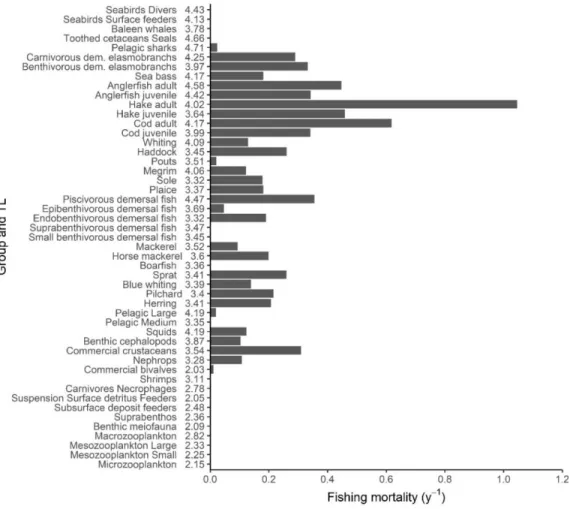
3.3. The MSY management scenario

The fishing mortality in the FMSY scenario is lower than in the status quo (Fstatus quo) for 6 of the 14 groups for which FMSY values are available (i.e. anglerfish, hake, cod, haddock, plaice and horse mackerel). In the FMSY scenario no group goes extinct (Fig. 9), despite the higher fishing

mortalities of trophic levels 3 to 4.3 (mainly pelagic fish) compared to the Status quo (Fig. 10). Mackerel biomass is, however, strongly depleted (3% of the Sc 0 biomass) and 6 groups have their biomass under 50% of the Sc 0 biomass. Compared to the Sc 1, the simulation predicts a positive impact on the biomass of predators (TL > 3.5) and a 32% increase in the total ecosystem biomass. Contrastingly, the biomass of preys is negatively impacted (-7% for TL 2.5 to 3.4) due to top-down control from predators and a higher fishing mortality. The FMSY strategy provides about the same amount of catch as in 2016 (1.54 t.km-2_{), which is 18% more than in the Status quo} scenario, and maintains high catches of horse mackerel and herring.

Fig. 9: Impact of the F

MSY

scenario (Sc 2) on functional groups biomass compared to the Sc 0,

colored bars indicate the amount of catch by group in the Sc 2.

21

3.4. Comparison between the F

MSY

scenario and the restricted BH strategies

The Sc 3 (BH TAC scenario) aims to balance F with P/B for the main commercial and assessed species. Similar to the FMSY scenario, all exploitation rates for this scenario (0.1, 0.25 and 0.4) lead to a decrease in the fishing mortality of predatory trophic levels (>3.5) (Fig. 11). The fishing mortality spectrum in the Sc 3 0.4 scenario is lower, but close to the FMSY scenario.

The lower F values of the Sc 3 0.4 generate less overall catch than the FMSY scenario (1.52 t.km-2_{) at Sc 3 0.1 (0.83 t.km}-2_{) and Sc 3 0.25 (1.32 t t.km}-2_{). The Sc 3 0.4 scenario predicts more} catch than the FMSY scenario (1.64 t.km-2), coming from groups at trophic levels smaller than 3.7

Compared to the Fmsy scenario, the 0.1 and 0.25 BH TAC scenarios induce a much smaller impact on the biomass of TLs above 3. In contrast, the 0.4 BH TAC scenario has a stronger negative impact on species at trophic levels above 3.7 than FMSY. Like in the FMSY scenario, the catches of the BH TAC scenario are dominated by horse mackerel (see supplementary).

Fig. 10: Trophic spectra of biomass ratio (right) of the Status quo (Sc 1, in red) and the F

MSY

(Sc 2, in gold)

compared with the No fishing scenario (Sc 0), and the catch compared with the F

MSY

scenario.

22

3.5. Incremental BH strategies

Balanced harvest on target fish species without TAC regulation

Applying a fishing mortality proportional to the productivity not only species under TAC regulation but also all other targeted groups (Sc 4) provides less catch than the Sc 3 scenario. In the Sc 4, FBH values are lower than Fstatus quo for most of the “target” groups except for pelagics. With an exploitation rate of 0.25 and 0.4 , this Sc 4 BH “targets” scenario has a stronger negative impact than the FMSY scenario on the biomass of predators (TLs>3.5) (Fig. 12 & 13) because of the increase of F on large pelagic fish (TL = 4.2).

Despite similar F spectra in the Fmsy scenario, and the BH Sc 3 and Sc 4 scenario at exploitation rates of 0.4, the latter two have a lower impact on the biomass of intermediate trophic

Fig. 11: Trophic spectra of fishing mortality, biomass ratio compared with the No fishing scenario (Sc 0) and

the catch ratio compared with the F

MSY

scenario of the BH TAC scenario (Sc 3) at 0.1 (dotted blue lines), 0.25

(dot-dashed blue lines) and 0.4 (solid blue line) exploitation rate and the F

MSY

(Sc 2, solid gold lines).

23 levels (TL 3-3.5). This is due to the shift in the fishing intensity from low productive species (demersal elasmobranchs, hake, cod) to high productive ones (medium pelagics, such as anchovy) in the BH strategies.

Balanced Harvest on bycatch fish species, targeted cephalopods and crustaceans

The scenario Sc 5 allows 1.5 times and 2.4 times more catches than the FMSY scenario (Sc 2) at 0.25 and 0.4 exploitation rates resulting from a high F on highly productive species (crustaceans and cephalopods). However, the exploitation rate of 0.4 leads to a low biomass of demersal species because of the loss in their prey, which are fished in this scenario, and the explosion of their main trophic competitors (i.e. pelagic groups and small demersal fish) (Fig. 12 & 13). The lower biomass of predators and the higher biomass of zooplankton have positive impacts on pelagic fish of intermediate trophic levels (3.3 – 3.6): they reach a higher biomass than in the unfished scenario Sc 0 (Fig. 12 & 13).

Full Balanced Harvest

At an exploitation rate of 0.1, the Full BH scenario impacts the biomass of TLs 3 to 5 less than in the FMSY scenario (Fig. 12 & 13). All function groups in this scenario recover to at least 60 % of their unfished biomass (Sc 0) (Supplementary II.4). The exploitation of very productive groups (e.g. macrozooplankton, bivalves) leads to high total catches (13.7 t.km-2_{). At 0.25 and 0.4} exploitation rates, this scenario produces even more catch, stemming from the exploitation of macrozooplankton (3.3 t.km-2_{)and benthos (15.3 t.km}-2_).

As in the Sc 5, Sc 6 as a lower impact on trophic levels 3 to 3.7 (pelagic fish)compared with the FMSY scenario but it has the strongest negative impact on high trophic level biomass among all the simulated scenarios. No groups go extinct in this scenario, but the cumulative effects of harvesting low trophic levels and high F on commercial species deeply impacts the biomass of demersal species which have less energy available and are still harvested.

24

Fig. 12: Trophic spectra of Sc 4 to 6 (Full BH) compared with the F

MSY

scenario at 0.1, 0.25 and 0.4 exploitation rate.

0.25 0.4

25

Fig. 13: Zoom of figure 12 on TL 3.5 to 5.

0.25 0.4

26

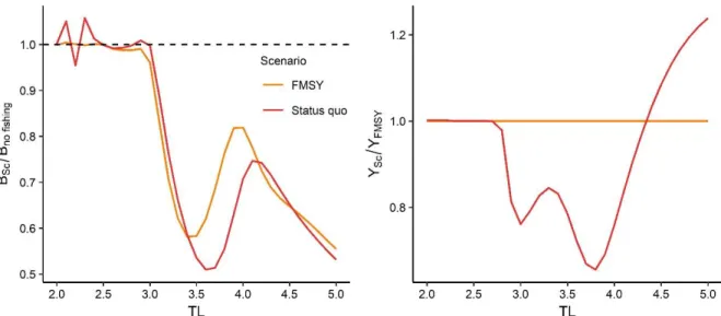
3.6. Ecological indicators

The ecological and catch indicators of the simulated scenarios show a clear difference between the conventional fisheries management scenario (Sc 1 and Sc 2) and the BH scenarios (Sc 3 to 6) (Fig. 14). Moving towards full BH would increase the total biomass of the Celtic Sea ecosystem, with a maximum of 98 t.km-2 _{for Sc 5 (BH bycatch and Invert.) with an exploitation rate} of 0.4. Compared to the FMSY scenario, broadening the range of harvested species increases the MTL of the system because of a strong increase in pelagic fish (Fig. 14 and Supplementary 2). At 0.25 and 0.4 exploitation rates scenarios Sc 5 and Sc 6 provide high catches (at 0.4, ~30 times more than in the FMSY scenario). But this catch has a very low mean trophic level MTLc (2.4) compared with other scenarios (next minimum is MTLc = 3.4), indicating that BH leads to catch manly composed of low trophic level species/biomass and thus low value species (benthic organisms and small fish). The 0.1 and 0.25 BH TAC scenarios show a strong decrease in the impact on the biomass of TL above 3 leading to the recovery of those trophic levels to values close the to the non-fished state and therewith to a more balanced biomass distribution (D = 1.5x10-5 and 8x10-5 _{respectively).}

Generally, all BH scenarios (Sc 3 to 6) at an exploitation rate of 0.4 are the least efficient in protecting high trophic level biomass (i.e. low HTI). In the BH scenarios, increasing the exploitation rate negatively affects both HTI and dispersion. Going towards full BH does not give a more balanced biomass structure, and leads to higher dispersion than the Status quo and FMSY scenarios. This high dispersion is linked to the relative biomass of TL from 2.5 to 3.5 that is diverging from the No fishing state. The BH bycatch & Invert. and the Full BH scenarios are performing better or equally well compared with the FMSY scenario only at an exploitation rate of 0.1, which results in 45 % less catch of predators (>3.5 TLs).

27

4. Discussion

4.1. Limits of the methods

All models are by definition a simplification of a complex reality. As any other ecosystem models, EwE is based on a set of assumptions that constrains its uses. For instance it assumes the diet is changing over time proportionally to prey abundance, while some parameters remain constant (like the Q/B ratio). This means some simulations outputs may be model-dependent and should ideally be compared with the ones from other models. In addition, our outputs may also

Fig. 14: Ecological indicator values of the Status quo, F

MSY

and BH scenarios.

The relative performance of each indicator is presented with a qualitative gradient from “bad” values (red)

to “good” values (green).

28 depend of the parameters we used, and which are often rather uncertain, while we were not able to develop sensitivity analyses, due to time constraints. Therefore, quantitative results of scenarios simulation have to be considered with care. However, our main findings are based on comparisons using rather qualitative than quantitative results.

On the other hand, EwE models are built in different ways to answer to various ecological or management questions (Plaganyi and Butteworth, 2004). The EwE model of the Celtic Sea ecosystem we used was built to assess effects of past fishing on primarly fish communities and ecosystem-based fisheries management scenarios. BH is one of the EAF possible scenarios that we tested in this study, but the construction of the EwE model limits the accuracy of our assessment. Indeed, among the 49 animal functional groups included in the model, 19 only are monospecies groups . The other groups are aggregation of different species that often vary highly in their abundance, production or productivity, while we were able to only simulate a mean global fishing pressure for the groups. This is not an issue when conventional fisheries management is tested but BH is designed to exert fishing mortality on the widest number of exploitable species in proportion to their natural productivity. Applying a fishing mortality proportional the productivity (P/B) of very productive multispecies groups is probably underestimating the effects of fishing than if species were modeled separately.

Froese et al. (2016b) also criticized ecosystem model approach to assess BH effects on ecosystems, because these models do not support BH. This come from the low trophic level groups that “carry” the top of the ecosystem leading to. I experimented this limit during my preliminary work: I introduced mesozooplankton groups in my Full BH scenarios. Even with low exploitation rate (0.1), harvesting these groups led to the mass extinction of all upper trophic level groups. Very low trophic level groups (e.g. zooplankton and benthic suspensivores) are often poorly represented in Ecopath model, and expected to remain unexploited when the model is used to simulate fishing scenarios. In other words, the model have been tested for realistic fishing strategies and appeared to provide reliable outputs in that case. Our work based on new and more contrasted scenarios highlights inconsistencies, suggesting the model has to be corrected, especially regarding some of the low TLs parameters

We used P/B as the key parameter to implement a fishing mortality for all the groups, in the same way some previous studies did (e.g. Garcia et al., 2011, 2012). Thus using the P/B value of the starting year (1985) to define fishing mortality and maintaining this fishing mortality constant over the whole simulation. This has to be considered an approximation, because P/B is changing over time as the ecosystem change (especially according to the predation mortalities in Ecopath),

29 and thus fishing mortality should do the same. .From a practical point of view, if BH becomes the management target changes in P/B would have to be assessed regularly and fishing mortality adjusted accordingly.

Zhou et al. (2019) suggested that BH could be also implemented by scaling the fishing mortality proportionally not to the productivity (what we did here) but to production (P). Heath et al. (2017) claimed that BH would be balanced only with F set according to P. This is also supported by the findings of Plank (2018), who used a multispecies predation model to test BH. However, we did not used this approach, because in an EwE framework, the value of P is strongly model-dependent, as building large trophic boxes leads to large P, while splitting a bow implies dividing the production. In addition, fishing mortality of each group should be recalculated every year according to production changes what would requires very complicated simulation based on the current Ecosim toolbox.

4.2. Status quo: still a lot to do for sustainable fisheries

The Celtic Sea has long been an area supporting important demersal fisheries, large and small pelagic fisheries and a variety of cephalopod and crustacean fisheries (Martinez et al., 2013). Pinnegar et al. (2003) demonstrated that commercial fisheries expansion in the past 50 years deeply affected the structure of fish communities and fisheries landings. The mean trophic level of both the catch and the animal community dropped as a result of the decline in the abundance of large piscivorous species; and the fisheries shifted from high trophic levels, and high priced species (e.g. hake, cod), to lower trophic levels, and lower priced species (e.g. blue whiting, mackerel) (ibidem). Moullec et al. (2017) further showed that the exploitation status of the Celtic Sea ecosystem did not improve significantly between 1980 and 2013, in spite of the reduction of the fishing pressure for some stocks (e.g. plaice, whiting, sole). Our study confirms what was previously found: the current fishing mortality pattern is not sustainable. In our status quo simulation hake, cod and horse mackerel go extinct. For these three stocks ratios between the fishing mortality of the status quo scenario and the FMSY scenario is high (reaching 3.75 for hake, a value that should probably be revisited in the model itself) suggesting that the current exploitation is far from fulfilling the objective of the Common Fisheries Policy to fish all stocks at FMSY by 2020 (Salomon and Holm-Müller, 2013). The current fisheries management is thus far from the target MSY approach and will lead to low catches and a low-quality ecosystem if sustainable fisheries policies are not applied and fishing mortalities were to remain constant.

30

4.3. The issue with targeting FMSY

The MSY concept exist since the 1930’ and has been criticized since the late 1970’s. It was described as the way of making “possible the maximum production of food from the sea on a sustained basis year after year” (Chapman, 1949). According to some authors, the MSY is a political choice using science to defend economic or geopolitical interests (Finley & Oreskes, 2013) and should be considered as a biological limit and not as a development target(Zhang et al, 2015).

The FMSY values we implemented were estimated by ICES from single species assessments,

which do not consider any ecological interactions between species and with the environment. The MSY concept is born from the old assumption that each fish stock can be managed in isolatation. In contrast, several studies demonstrated that the single-species MSY approach can lead to overexploitation of stocks due to depensatory effects from predator prey interactions (Brander and Mohn, 1991; Pauly et al, 2002; Walters et al., 2005). In our Ecosim model, considering the current range of harvested species, the FMSY scenario fulfills its catch maximization objectives and maintains the stock biomass at higher levels compared with the Status quo scenario. It also shows that reducing the fishing mortality of high value predator species (e.g. sea bass, hake, cod,

anglerfish) could provide more catch of these species in the long-term (0.124 t.km-2 _vs 0.104 t.km-2 _{in Status quo) while improving slightly the relative abundance of high TLs species}

(HTI +0.05). However, the MSY approach does not rebuild the biomass structure of the ecosystem which remains unbalanced and several groups can’t recover (horse mackerel: 39 % of unfished system biomass, whiting: 25 %, sea bass: 13%, mackerel: 0.06%). In addition, applying the MSY approach only to species that are currently under TAC regulation (the only one where FMSY has been currently estimated) results in several groups can’t recover (horse mackerel: 39 % of unfished system biomass, whiting: 25 %, sea bass: 13%, mackerel: 0.06%).

More generally, the MSY approach is leading to a strong impact on each exploited stock (i.e. an exploited biomass divided by 2.5 or 3), with long term or ecosystems effects that are poorly known, and thus no guaranty it will be compatible with the conservation of the functional and genetic diversity of ecosystems (Gascuel, 2019).

31

4.4. Balancing the harvest of main caught species, the solution?

In the Sc 3 “BH TAC scenario” we balanced fishing mortality proportionally to the productivity of all species under TAC regulation. This scenario is the simplest and ad minima implementation of a balanced harvest approach, just needing information on the productivity (P/B) of those stocks/populations that are already fully assessed by ICES. At an exploitation rate of 0.1, this scenario is the most sustainable overall, leading to good indicators and low impact on predators. But it would decrease the total catch by 45 %, which would have important negative impacts on the fisheries economy in the area. For example, hake catch would decrease about 68 %, representing a loss of 92 € km-2_{, and 22 million € at the Celtic Sea scale (if the price remains at} 3.69 € kg-1_{, European market observatory for fisheries and aquaculture products (EUMOFA),}

2017). By contrast, at an exploitation rate of 0.25, the Sc 3 scenario leads to limited loss of catches

(-13 %).The FBH values are generally still lower than the FMSY (-35% on average) but FBH 13 % higher for blue whiting and 43 % for sprat than their respective FMSY.

At a 0.4 exploitation rate, it could be possible to keep an acceptable level oflarge total catch, which would be more than the FMSY scenario (+0.11 t.km-2). In addition, harvesting 40% of the productivity of the currently targeted species would have less impact on the total biomass structure than the FMSY scenario. However, the fishing mortality in this scenario will be higher than FMSY for hake, anglerfish, cod, haddock, plaice, sprat and blue whiting, which is against all management measures that are applied in Europe since the 90’s. FurthermoreMore generally, this scenario leads to strong impacts on high TL species (low HTI), which is likewise not considered as acceptable. The FMSY values are probably overestimated because of the ecological assumptions behind it, and should represent a maximum harvest barrier. On the other hand, harvesting 40% of the productivity of the currently targeted species would have less impact on the total biomass structure than the FMSY scenario. BH on species under TAC regulations at a 0.4 exploitation rate, has and exhibit the lowest worse ecological indicator values.. In other worlds, BH TAC would be thuscould be considered as ecologically sustainable and acceptable only with moderate exploitation rates. However, it would imply a reduction of catch compared to the Status quo and FMSY scenarios and therewith would not fulfill one of the central promises of BH: the provision of significantly higher sustainable catches (Garcia et al., 2012). For this balanced harvest needs to be implemented on a wider range of species.

32

4.5. Toward full balanced harvest: successes and failures

None of our balanced harvest implementations could fulfill the promises made by most of the BH advocates: maintaining and rebuilding the ecosystem structure, while catching more fish (Zhou et al., 2010 ; Garcia et al., 2012). We explored BH on different ranges of species, from the most feasible (BH target scenario) to the more technically difficult (Full BH). None of them resulted in biomass structures similar to the unfished system (Sc 0). Within all scenarios, the BH target scenario (Sc 3) using an exploitation rate of 0.1 is also the one with the lowest fishing mortality on all trophic levels and it led to the lowest dispersion and the highest HTI. Adding other groups to the harvested range, or increasing the exploitation rate, always led to higher catch and higher dispersion (thus less balance impacts).

Quite surprisingly, moving towards a full BH implementation (Sc 5, BH bycatch invert. &; Sc 6 ,Full BH) with high exploitation rates increased the total biomass and the MTL. The total biomass increases were due to the depletion of predators that caused the positive impacts on low trophic level groups (around 2.6 and 3.5), such as small pelagic fish (blue whiting, sprat and boarfish).

When adding benthic invertebrates to the exploited species (Sc.6), the total biomass still increase a bit, due to the increase of some low or intermediate TL groups (mesozooplankton at TL 2.6 and sprat, blue whiting, boarfish and herring at TL 3.3). This result illustrate a strong limit of BH in practice. Because exploiting all the numerous species that have a low or intermediate TLS in not feasible technologically speaking (and even less adjusting F to the species productivity), expending the range of exploitation will necessarily lead to unbalanced effects, little or no exploited species benefiting from a competition pressure decrease.

Another outcome from these simulations is the strong negative impact on high trophic levels (> 3.8-4). The most intense (0.25 and 0.4) scenarios show a very low HTI, owing to the depletion of the biomass of apex predators. At an exploitation rate of 0.4, the fishing mortality of trophic levels 3.5 to 5 is higher than in the FMSY scenario. In contrast, at an exploitation rate of 0.25, the F on high TLs is lower than in the FMSY scenario, but nevertheless causes a stronger depletion of high TL biomass. We suggest this result to be the combined effect of fishing on predators and the cumulative impact of harvesting their preys. Following the basics of thermodynamics, losses of biomass and energy from fishing at the bottom of the trophic pyramid results in less available biomass and energy for the top of the pyramid. In line with this Smith et al., (2011) showed that

33 fishing low trophic levels at MSY would have deep impacts on higher trophic levels. Our results confirm these effects and the concern put forward by Froese et al. (2016) that BH might increase the systems biomass and yield, but that this could mask cumulative negative changes in the food-web structure.

Our simulations of an acceptable Full balanced harvest implementation contradict what has been claimed in the literature: It does not lead to a balanced biomass distribution, except when fishing intensity is low and therewith fisheries production (0.1 exploitation rate). In the Full BH implementation with exploitation rates of 0.25 and 0.4 provide large catches but also show strong impacts on the biomass of predators. The exploitation rate is well balanced across trophic levels in our scenarios but the biomass is still not balanced. Bundy et al., (2005) also found in the case of the Eastern Scotian shelf and the Gulf of Thailand Ecopath models that balanced exploitation (i.e. BH) led to less dispersion but to lower diversity when exploitation rate was above 0.28. The decrease of MTL induced by a Full BH implementation with exploitation rates of 0.25 or 0.4 4 is stemming from large increases in low and intermediate trophic level species, particularly of pelagic fish biomass. The changes in the relative abundance of pelagic fish and demersal fish could make the ecosystem more sensitive to environmental variations and less resilient (Fréon et al., 2005).

The first lesson to take away is that none of our BH scenarios led to biomass structures similar to the unfished ecosystem, as was proposed in the literature (Zhou et al., 2019). The only way to approach the balance of the biomass structure is to fish at very low intensities and therewith reduce drastically the catch on the system.

A full balanced harvest implementation with low exploitation rates (0.1) appears to be the upper limit for such strategy for the Celtic Sea case study. But it implies a lot of disadvantages. First, we have to accept that if we want to fish more and rebuild stocks, fisheries have to shift from the current target species, which are mainly demersal with low productivity (e.g hake, anglerfish) to more productive species (e.g. small demersal fish, zooplankton). Furthermore, such shift would have strong impacts on high trophic levels (>4) due to cumulative effects of energy loss. Finally it may induce some unbalanced effects on low or intermediate TLs, where it is practically not feasible to adjust the fishing mortalities to each species productivity.

Moving towards a full balanced harvest implementation would require a radical restructuring of fisheries, market and even customers behavior. BH implies to harvest and sell tons of not yet commercial species, like zooplankton, small demersal fish and benthic organisms. Zooplankton harvesting already exists but is restricted to Krill in Antarctica and the North Pacific, Calanus