STUDY OF THE TRAJECTORIES OF ICE SHED BY
DEICING SYSTEM AROUND AIRCRAFT ENGINE
by
Hassan EL SAHELY
THESIS PRESENTED TO ÉCOLE DE TECHNOLOGIE SUPÉRIEURE IN
PARTIAL FULFILLMENT FOR A MASTER’S DEGREE WITH THESIS IN
ENGINEERING CONCENTRATION AEROSPACE
M.A.Sc
MONTREAL, DECEMBER 12, 2019
ÉCOLE DE TECHNOLOGIE SUPÉRIEURE UNIVERSITÉ DU QUÉBEC
©Tous droits réservés
Cette licence signifie qu’il est interdit de reproduire, d’enregistrer ou de diffuser en tout ou en partie, le présent document. Le lecteur qui désire imprimer ou conserver sur un autre media une partie importante de ce document, doit obligatoirement en demander l’autorisation à l’auteur.
BOARD OF EXAMINERS
THIS THESIS HAS BEEN EVALUATED BY THE FOLLOWING BOARD OF EXAMINERS
Mr. François Morency, Thesis Supervisor
Department of Mechanical Engineering, at École de Technologie Supérieure
Mr. Stéphane Hallé, President of the Board of Examiners
Department of Mechanical Engineering, at École de Technologie Supérieure
Mme Marlène Sanjosé, Member of the jury
Department of Mechanical Engineering, at École de Technologie Supérieure
THIS THESIS WAS PRESENTED AND DEFENDED
IN THE PRESENCE OF A BOARD OF EXAMINERS AND PUBLIC ON DECEMBER 03, 2019
ACKNOWLEDGMENT
This thesis is done through two years in which professor Francois Morency played an essential role in supervising and advising me to the correct path by his intelligent ideas. I am grateful and thankful to him. I would like to thank all the members of TFT laboratory for their continuous support specially Abdallah, Olivero, Kevin, Sami, Sébastien, Violaine, Gitsuzo and Ahmed. I would like to tell them that your effort is highly appreciated.
I would like to thank god in the first place for giving me the power and strength to achieve this work. Also, my small family was supportive emotionally and financially and without them it’s impossible to achieve what I am now. I want to tell my parents it’s time to be proud of your son.
Étude des trajectoires des particules de glace par système de dégivrage autour du moteur de l’avion
Hassan EL SAHELY
RÉSUMÉ
Le problème de l’accumulation de glace a causé des accidents et des incidents aux aéronefs au cours des dernières décennies. La résolution du problème de l’accumulation de glace à l’aide de dispositifs de dégivrage et d’antigivrage permettra d’éliminer la glace accumulée, mais le problème des trajectoires inconnues des particules détachées apparaît. Les particules de glace représentent un grand danger pour l’aéronef. Le risque varie en fonction de la vulnérabilité des pièces de l’aéronef. Les parties vulnérables de l’avion sont l’aile, le fuselage arrière, les stabilisateurs et les moteurs montés à l’arrière. Afin d’atténuer le risque, une étude des trajectoires des particules est introduite. L’objectif de cette recherche est d’étudier les trajectoires autour d’une aile en changeant l’angle d’attaque et l’angle de flèche. Le but est de calculer le nombre minimal de trajectoires de glace pour prédire correctement une carte d’empreinte à la section d’entrée du moteur en utilisant la méthode de Monte-Carlo. Une approche numérique est utilisée pour réaliser cette étude. Les trajectoires aléatoires des particules de glace sont calculées à l’aide d’un champ de vitesse calculé par la méthode des panneaux 3D (3DPM). Pour déterminer les zones derrière l’aile où les particules de glace ont la plus grande probabilité de passage, une méthode de Monte-Carlo est utilisée. Dans cette recherche, les calculs sont effectués au moyen d’une étude probabiliste des empreintes pour déterminer la forme de leur distribution de probabilité. Une fois la forme connue, un test de normalité est effectué sur la forme de la fonction de distribution de probabilité (PDF) appelé le test Kolmogorov-Smirnov. Après avoir déterminé la forme et le type des PDF, une étude sur la moyenne et la variance pour chaque PDF est effectuée pour vérifier le nombre minimal de trajectoires nécessaire pour la méthode de Monte-Carlo. Le champ d'écoulement de 3DPM est validé par rapport à la littérature ainsi qu’à la répartition de l’empreinte derrière l’aile. L’effet de l’angle d’attaque, ainsi que l’angle de flèche sur les trajectoires de particules de glace, est montré. L’augmentation de l’angle d’attaque déplace les trajectoires vers le haut tandis que la flèche rend la carte d’empreinte moins bruitée. Enfin, 500 trajectoires sont suffisantes pour prévoir une carte d’empreinte.
Study of the trajectories of ice shed by deicing system around aircraft engine
Hassan EL SAHELY
ABSTRACT
The problem of ice accretion caused accidents and incidents to aircraft over the past decades. Solving the problem of ice accretion employing de-icing and anti-icing devices will remove the accumulated ice but the problem of unknown trajectories of the detached particles appears. The flown particles represent a great hazard on the aircraft which yields risk depending on the vulnerability of aircraft parts. The vulnerable aircraft parts are the wing, the rear fuselage, the stabilizers, and the rear-mounted engines. In order to mitigate the risk, a study of the trajectories of those particles is introduced. The objective of this research is to study the trajectories around a wing by changing the angle of attack and the sweepback angle. The goal is to calculate the minimal number of ice trajectories to correctly predict a footprint map at the inlet section of the engine using the Monte-Carlo method. A numerical approach is used to accomplish this study. The random trajectories of the ice particles are calculated using a 3D Panel Method (3DPM) flow field around the wing. To determine the zones behind the wing where the ice particles have the most passage probability, a Monte-Carlo method is utilized. In this research, the calculations are done through a probabilistic study of the footprints to determine their probability distribution's shape. Once the shape is known, a normality test is done on the shape of the Probability Distribution Function (PDF) called the Kolmogorov-Smirnov test. After determining the shape and the type of the PDFs, a study on the mean and variance for every PDF is done to check the minimal number of trajectories to fulfill the Monte-Carlo method. The 3DPM flow field is validated against the literature as well as the footprint distribution behind the wing. The effect of the angle of attack, as well as the sweepback angle on ice particle trajectories, is shown. The increase of the angle of attack shifts the trajectories upward while the sweepback makes the footprint map less noisy. Finally, 500 trajectories were found enough to predict a footprint map.
TABLE OF CONTENTS
Page
INTRODUCTION………...………….1
CHAPTER 1 REVIEW OF LITERATURE ...5
1.1 Flying in icing conditions ...5
1.2 Ice-particle trajectory simulation ...7
1.3 Ice shed computation methods ...9
1.4 Monte-Carlo simulation on trajectories ...11
CHAPTER 2 MATHEMATICAL MODELING AND NUMERICAL METHOD ...15
2.1 3D panel method ...15
2.1.1 3D potential flow over a wing ... 15
2.1.2 Solution by Green’s identity ... 16
2.1.3 Dirichlet boundary conditions... 18
2.1.4 Influence coefficient calculation ... 19
2.1.5 Computations of surface velocities and pressure ... 22
2.1.6 Velocity calculations in the farfield ... 24
2.1.7 Closing the wing tip ... 25
2.2 Trajectories simulations ...29
2.3 Monte-Carlo Simulation ...36
2.4 PDFs estimator ...38
2.5 Code implementation ...39
CHAPTER 3 RESULTS AND DISCUSSION ...41
3.1 Validation and verification ...41
3.1.1 Wing tip closure effect ... 41
3.1.2 Trajectories verification ... 43
3.2 Monte-Carlo simulation ...48
3.2.1 Effect of angle of attack ... 49
CONCLUSION………...………71
ANNEX I……….………….73 LIST OF BIBLIOGRAPHICAL REFERENCES ...77
LIST OF TABLES
Page Table 3.1 Initial conditions for Suares simulations...47 Table 3.2 Wing and flow field characteristics for Monte-Carlo method ...49
LIST OF FIGURES
Page
Figure 0.1 Inflight icing on the non-protected surfaces (Bremmer, 2018) ...1
Figure 1.1 Ice particles detaching from the wing leading edge experimentally by NASA using electro-expulsive system. ...6
Figure 2.1 Potential flow around a solid body inspired by Katz et Plotkin (2001) ...17
Figure 2.2 Quadrilateral panel (Katz & Plotkin, 2001). ...20
Figure 2.3 Kutta condition at the trailing edge (Katz & Plotkin, 2001) ...21
Figure 2.4 Panel local coordinate system to evaluate the tangential velocity components ...23
Figure 3.1 Total lift coefficient comparison between the software XFLR5 and panel method code for flow correction ...42
Figure 3.2 Comparison between the current panel code and the software XFLR5 for the pressure coefficient at AOA = 5° and different numbers of panels. ...43
Figure 3.3 Pressure coefficient comparison between 3DPM code and experimental results ...44
Figure 3.4 Pressure coefficient comparison at AOA = 0°. ...45
Figure 3.5 XZ view of the trajectories. ...46
Figure 3.7 Probability distribution of the trajectories at x = 2c plan behind
the wing at AOA = 4° with NACA23012 airfoil. ...48 Figure 3.8 Variation of trajectories footprint with respect to the angle of
attack SBA = 0°, number of trajectories = 200. ...51 Figure 3.9 Variation of number of trajectories footprint, AOA=5°, SBA=0°. ...52 Figure 3.10 Rotation of the view ...53 Figure 3.11 3D probability distribution of the footprint trajectories for 500
trajectories at AOA = 5° and SBA = 0°. ...54 Figure 3.12 Probability distribution of the trajectory’s footprint with respect
to the z-axis. ...55 Figure 3.13 Cumulative probability distribution for P(Z) for 500 trajectories (a)
and 1000 trajectories (b). ...55 Figure 3.14 Mean variation vs number of trajectories for P(Z). ...56 Figure 3.15 Variance variation vs number of trajectories for P(Z) ...57 Figure 3.16 Probability distribution of the trajectory’s footprint with respect
to the y-axis. ...58 Figure 3.17 Cumulative distribution function for P(Y) for 500 (a) and 1000 (b)
trajectories. ...58 Figure 3.18 Mean variation vs number of trajectories for P(Y). ...59 Figure 3.19 Variance variation vs number of trajectories for P(Y). ...60 Figure 3.20 Variation of trajectories footprint with respect to the sweepback
XVII
Figure 3.21 Variation of number of trajectories footprint at plan = 6.5 m,
AOA = 5°, ...63 Figure 3.22 Probability distribution of the trajectory’s footprint with respect
to the z-axis. ...64 Figure 3.23 Cumulative distribution function for 500 (a) and 1000 trajectories (b). ....65 Figure 3.24 Mean variation vs number of trajectories of P(Z), SBA = 30°,
AOA=5°. ...66 Figure 3.25 Variance variation vs number of trajectories of P(Z), SBA=30°,
AOA=5°. ...66 Figure 3.26 Probability distribution of the trajectory’s footprint with respect to the y-axis. .67 Figure 3.27 Cumulative probability distribution for P(Y) for 500 (a) and 1000 trajectories
(b). 67
Figure 3.28 Mean variation vs number of trajectories P(Y), SBA=30°,
AOA=5°. ...68 Figure 3.29 Variance variation vs number of trajectories P(Y), SBA=30°,
LIST OF ABREVIATIONS
CFD Computation fluid Dynamics
BWB Blended Wing Body
3DPM 3D Panel Method
GA Ground Aviation
CFR Code Federal Regulation
2D Two dimensional
3D Three-dimensional FAA Federal Aviation Administration
NASA National Aviation and Space Administration PDF Probability Distribution Function
TFT Laboratory of ThermoFluide pour le Transport
AR Aspect ratio
DOF Degree of freedom
CP Centre of pressure
CG Center of gravity
MATLAB Matrix Laboratory
SR Surface Ratio
SBA Sweepback angle
AOA Angle Of Attack
AOPA Aircraft Owners and Pilots Association NTSB National Transportation and Safety Board
LIST OF SYMBOLS
Φ Potential flow velocity
𝜎 Source strength
𝜇 Doublet strength
ζ The skid angle
c Chord
I Inertial matrix of the flat plate
P, Q, R Angular velocity of the debris particle in the three axis of rotation
m Mass of the particle
Vre Relative velocity
α Angle of attack
β Side slip angle
Fnp Normal resultant force on the particle
D Drag force
L Lift force
L, l, e Length, width and thickness of the particle
g Gravitational force
Cdm Coefficient of dynamic moment
CN Normal resultant force coefficient
N Total number of trajectories
h Bandwidth coefficient
Up, Vp, Wp Velocity components of the particle in the global frame of reference 𝑢 , 𝑣 , 𝑤 Velocity components of the particle due to source
𝑢 , 𝑣 , 𝑤 Velocity components of the particle due to doublet ε Error
q1, q2, q3, q4 Quaternions
𝛺 Vector rotation of the flat plate Xc, Yc, Zc Coordinates of the collocation point
INTRODUCTION
The problem of icing on wings is a serious problem in aviation. The ice accretion on the wing’s leading edge increases the drag and disturbs the smooth air around the wing, thus destroying lift creation (FAA,2008). Flying in such conditions will cause hazards for the aircraft, leading to emergency descent or crash. The problem of ice accretion on wings has caused many incidents and accidents recorded over the past three decades. For example, the Embraer EMB-500 Phenom 100 on December 8, 2014, crashed because of the ice accretion on the wing caused the aerodynamic stall (NTSB,2016). Figure 0.1 shows an illustration of an aircraft with an iced wing (Bremmer,2018). It demonstrates the perturbation of the flow around the lifting surface. This flow perturbation is shown in the picture by the streamlines in blue color.
Figure 0.1 Inflight icing on the non-protected surfaces (Bremmer, 2018)
12 % of the total crashes related to weather conditions according to 10 years statistics between 1990 and 2000, were linked to icing (AOPA,2008). Moreover, in the four years between 2010 and 2014, the National Safety Transportation statistics reported many major accidents. The 52 recorded accidents led to 78 fatalities (AOPA,2008). To avoid these types of incidents and accidents, ice accumulation could be eliminated in two ways: either by deicing systems or with
anti-icing systems. Deicing removes the ice accretion after being accumulated, but anti-icing prevents any ice accretion on the aircraft surfaces. One of the solutions suggested to remove the ice accumulated inflight is a flexible membrane on the leading edge called a “Flexible rubber boot” (FAA,2008). This membrane expands and contracts, to remove the accumulated ice on the leading edge (FAA,2008).
The ice accreted on the leading edge is detached employing de-icing devices. Some particles will hit the aircraft and the majority will fly downstream the flow. While flying, the ice particles detached from the wing leading edge will transform into a flying hazard. It can cause damage to the aircraft parts such as the fuselage, stabilizers or the rear mounted engines. The manufacturers take into consideration the hazard of flying ice particles in order to minimize their probability of being ingested by the engines (Suares,2005). If the ice particles strike the engine, serious damage will occur to the fan blades and other engine parts (Morse,2004).
The goal of this work is to build a tool that enables quick study of the wing geometry on footprint maps. In this study, a numerical method is used to simulate the trajectories of the ice particles. The method used to obtain the flow field around the wing is a 3D based panel method (3DPM), that uses source and dipole singularities. Previous studies used 3D computational fluid dynamics (CFD) and computational domain around a geometry to calculate the velocity flow field in the near and farfield such as (Papadakis et al, 2007), (Ignatowicz et al., 2019), (Deschenes, Baruzzi, Lagace, & Habashi, 2011), (Suares,2005). All these studies used a CFD mesh to discretize the volume around the aircraft. The CFD method calculates the three components of the fluid velocity at all nodes of the mesh. The trajectory is calculated based on Newton’s second law of motion by interpolating velocity from the computed CFD solution at each node. One of CFD negatives is the difficulties of mesh generation which requires skills and time. After generating the mesh depending on its size, the flow solution should be generated as well. When the mesh is finer, then the interpolation between the nodes to find the velocity will require even more time. But in 3DPM the solution is generated quickly. The 3DPM asks only for the airfoil coordinates then the surface mesh is directly generated.
3
The trajectories can cross a certain plane after the wing, perpendicular to the fuselage (it will be specified in the methodology section). At this specific plane, the footprints of the trajectories will be collected. The collected footprints form an icing footprint map. To well predict the footprint map of the ice particles, a Monte-Carlo method should be used (Papadakis et al., 2007). To perform this approach a huge number of trajectories should be simulated. The main challenge facing the Monte-Carlo method is the computation time for the trajectory’s calculation. The objective of this research is to perform a Monte-Carlo approach with a reduced number of trajectories by assuming a specific shape of the probability distribution function (PDF) of the footprints at the plan of interest. The proposed method only needs a surface mesh of the solid body to compute the flow field. The 3D Panel Methods ables to computes the velocity at all points on the surface of the solid body (wing) and in the farfield. The calculation of the trajectories is based on the Newton’s second law of motion in the Lagrangian frame of motion. Moreover, for the calculation of the resultant aerodynamic force, the aerodynamic coefficient must first be calculated, taking into account local angle of attack and side slip angle of the particle through correlations, instead of calculating all aerodynamic forces at each time. A 3D dynamic moment and static moment are also applied to the particle (rectangular flat plate in this case) since the particle rotates while moving. The PDF should be evaluated based on the footprint map data. Thus, the data are fitted in a fitter app to check their PDF shape. For every number of trajectories simulated, a shape of the correspondent PDF is obtained and tested. The shape of the functions is then compared. After that, a study of the PDF characteristics is done to show the optimal number of trajectories needed to fulfill Monte-Carlo approach by changing the angle of attack and the sweepback angle.
This thesis is divided into three chapters. In the first chapter, a review of literature is conducted to reveal the state of the art of this research with respect to previous researches in the same domain. The first chapter starts considering the inflight icing conditions and how flying in such conditions could adversely affect the aircraft. In addition, computations of the ice trajectories using CFD and 3DPM flow field from the literature are illustrated. Moreover, trajectories simulation techniques are exposed. Finally, an illustration of the Monte-Carlo approach used for ice-particle simulations is carried out.
Chapter two will present the methodology of this research. The equations used in the mathematical model are implemented into a MATLAB code to compute the trajectories in a non-uniform flow field. Also, in this chapter, an algorithm is proposed to close the wingtip of the grid used in order to correct the flow field around the wing. Finally, the Monte-Carlo approach with an assumed probability distribution function is presented.
Chapter three will present the results of this study. A validation of the flow field is done against the experimental data. A comparison with the literature reveals a verification of the proposed methodology as well as a validation with Suares (2005). A Monte-Carlo study is done to compute the probability distribution of the trajectories at a plan downstream of a wing. The effect of the angle of attack will be investigated as well as the sweepback angle. Finally, A probabilistic study will be performed to check the correct number of trajectories computation needed to fulfill the Monte-Carlo study.
CHAPTER 1
REVIEW OF LITERATURE
This section presents a review of the studies done in the literature related to the domain of aircraft de-icing. This review is classified into four sub-sections: Flying in icing conditions, ice particle shedding simulation, ice shed computation method and Monte-Carlo simulation on trajectories.
1.1 Flying in icing conditions
During flight, especially where the temperature is near the freezing point and below, ice may accrete on the non-protected surfaces of the aircraft and may lead to degradation of the wing performance (Cebeci & Besnard, 1994). The saturated clouds form a layer of ice on the surface of the wing’s leading edge, nose and fin. There are many numerical and experimental models for ice formation presented in the literature (horn ice, rime ice, glaze ice), (Cao, Zhang, & Sheridan, 2019), (Papadakis, Yeong, Wong, Vargas, & Potapczuk, 2005). The ice formed could be de-iced locally on the aircraft parts by different methods: mechanically, either by using a flexible membrane which inflates or mechanical actuators (Venna & Lin, 2006), and electrically by applying an electric current to heat up the surface and detach the buildup ice (Giamati, Leffel, & Wilson, 1995). Others like Petrenko (2010), used a combination of an electrothermal and electromechanical deicing system. The detachment of the ice will solve the problem of wing reshape to gain back its performance, but it results on appearance of another problem, which is the random trajectories of those particles. The detached particles have random shapes volumes and masses, and may strike the aircraft parts like windows or rear-mounted engine (Mason, Strapp, & Chow, 2006) that lead to fatal consequences.
Petty et Floyd (2004) presented a statistical study on aircraft icing accidents. The accidents due to ice accumulation on the airframe are grouped into three categories: GA (General Aviation), 14 CFR (Code Federal Regulation) Part 135 and Part 121. Petty et Floyd mentioned that 583 accidents were recorded between 1982-2000. The accidents lead to 819 fatalities according to
National Transportation and Safety Board (NTSB) in Washington DC. The NTSB’s study also showed that the percentage of aircraft accidents, due to icing, depends on the flight phase. The study deduced that the highest accident percentage was found in the cruising flight phase.
To study and test ice accumulation on aircraft parts is not an easy task. To check how the aerodynamic forces on the aircraft changes, experimental tests should be done. Figure 1.1 shows the ice particle detachment from the wing leading edge. This experiment was done by NASA. It shows clearly how the trajectories of the ice pieces possess different shapes. The trajectories of the ice particles goes the same direction as the flow.
Figure 1.1 Ice particles detaching from the wing leading edge experimentally by NASA using
electro-expulsive system.
Aircraft manufacturers and aviation authorities try to predict the problem of ice accretion for risk mitigation. This aspect is expensive and cost the aircraft manufacturer a lot. In fact, tests in wind tunnel, for example like the experiments done by Papadakis et al., (2007), under specific icing conditions could be less expensive than doing the same test inflight. Going toward computer simulations may be a good solution as well to minimize the study costs. These
7
simulations could give results with excellent agreement with the experimental data if they are well performed.
1.2 Ice-particle trajectory simulation
Some researchers have modelled the ice shedding problems and proposed ways to estimate the danger in some regions downstream of the main aircraft parts. This section highlights the most relevant previous studies about ice shedding.
One of the first researches in the panel method for 2D and 3D meshes was done by Hess et Smith (1967) for Douglas company. This method was revolutionary at that time because it was able to predict correctly the flow field around an arbitrary body. Later, Katz et Plotkin (2001) explained also the panel method for 2D and 3D based on Hess and Smith. NASA in 1991 published research about developing the PMARC program which was based on the 3D panel method (Ashby, Dudley, Iguchi, Browne, & Katz, 1991). These methods compute the flow field around the solid body and enable the calculation of the flow field parameters for trajectories calculation.
Kohlman et Winn (2001) studied the ice pieces trajectories of a particle with 4-DOF (three translational and pitching angle) in a uniform flow field. The ice-piece is a square with a uniform thickness shed from the fuselage. The initial angle of attack, the damping coefficient and the thickness of the plate were predefined as initial conditions. The main model is based on the Newton’s second law of motion. Aerodynamic forces (lift and drag) on the square are calculated from aerodynamic coefficients. The aerodynamic coefficients are calculated using correlations that depend on the angle of attack and the rotation velocity. A sensitivity study was conducted to determine the effect of the size and the thickness of the shed ice shapes. The results show that the ice piece rotation depends on the damping coefficient and the angle of attack. Also, the trajectory position is obtained by varying the following parameters: the size of the ice-piece, the damping coefficient, the thickness of the particle and the angle of attack.
Santos, Papa, et Do Areal Ferrari (2003) simulated ice trajectories based on CFD solution from FLUENT. The trajectory calculation is based on correlations for aerodynamic coefficients obtained from the literature. The whole methodology was based on the one proposed by Kohlman et Winn (2001). The study was limited to a number of parameters: the angular velocity, the initial angle of rotation, and the pitch damping coefficient. The ice shedding was from a fixed location x = -0.1 m, y = 0.1 m and z = 0.1 m. The results show the probability distribution at the plane x = 8 m after the wing in a 0.5 m discretization along the z-axis. They used a low number of trajectories of 343. The addition of Santos to Kohlman’s work is that the methodology of Santos was combined with CFD flow field results in order to evaluate the risk of impact of the ice pieces at specified areas in a cross-section plan downstream the flow.
The windborne debris trajectories has been studies in the field where the impact of hurricanes should be studied. Holmes, Letchford, et Lin (2006) conducted a 2D simulation of the debris trajectories. Their study was done numerically and experimentally in the wind tunnel at Texas Tech University. They used only a square plate as a representation of the debris but with various dimensions. The calculations of the lift, drag and moments applied to the debris were calculated based on aerodynamic coefficients, which are function of the angle of attack. The trajectory of the debris was calculated by means of the Newton’s second law of motion in a uniform flow field. Holmes compared the results with the results obtained by Tachikawa (1983). The results show a comparison of the trajectories with and without Magnus effect. The Magnus effect is the rotation of the particle caused by the fluid motion which creates additional lift force. This additional lift force could be positive or negative depending on the initial angle of rotation the debris. The normal force coefficient, the center of pressure position, and the Magnus effect lift showed their importance for trajectories computations.
Kordi et Kopp (2009) used Newton’s second law of motion to predict trajectories of flat plates in a uniform flow field. The model is based on dimensionless initial parameters: rotational lift, drag, pitching moment and velocity. The Magnus effect was considered. The autorotation of the plate was taken into account as a single degree of freedom system experimentally to estimate onset of the autorotation, the tip speed and the coefficient of the forces. The results
9
were compared to the experimental results obtained by Tachikawa (1983). The aspect of this study focused on the asymptotic limits of the dimensionless rotational, vertical and horizontal speeds as function of the geometry as well as the aerodynamic forces. Kordi and Kopp noticed that the dimensionless parameters governing the trajectories of the debris are the angular velocity, the pitching angle, the rolling angle, and the thickness ratio of the particle.
1.3 Ice shed computation methods
Many scientific papers study the ice-particles trajectories after detachment from the wing. The 3DPM can calculate the flow field around the solid body necessary for trajectories computations (Chandrasekharan & Hinson, 2003). The other method for trajectories computation uses CFD flow field solutions using two different types of meshes: dynamic mesh like Baruzzi, Lagacé, Aubé, et Habashi (2007) and static mesh like Ignatowicz, Morency, et Lopez (2019). This section illustrates the various flow field solution methods developed for ice shedding.
Chandrasekharan and Hinson (2003) studied the ice trajectories around the Learjet 40 and Learjet 45 Bombardier aircrafts for certification. The study was carried out numerically using the 3DPM implemented in the VSAERO code to provide a necessary flow field around the solid object. Moreover, they modified the ICE program which simulated water droplet to be able to simulate solid ice particles. The location of the ice shed was specified to be the nose of the two aircrafts since the fuselages are different in length. The ice fragment wasn’t chosen to shed from the wing since both aircraft has similar relative distance between the wing leading edge and the engine inlet section. For this test, the parameters to be varied are the aircraft speed, the angle of attack and the ice particle size. Relying on experimental tests, those variables were selected to study their effects on the ice trajectories. The study deduced that the ice trajectories are not affected by the fuselage length difference. The experimental test agreed with the numerical test which help decrease the simulations cost. The experimental test done on the aircraft wasn’t mentioned on Chandrasekharan and Hinson paper.
Baruzzi et al. (2007) developed a new method for ice shed trajectories simulation in a uniform flow field using CFD. The study was based on Navier-Stokes analysis solved with an implicit linearization and a finite element discretization. The concept of the simulation is based on moving sub-mesh inside the main mesh connected by stitching. This is called a dynamic mesh. At each time step, the channel (it is a square sub-mesh grid represents the ice-particle) detach and by computing the new position of the particle, the channel is repositioned and reconnected to the whole domain with the removal of all overlapping. This numerical approach computes the forces in the same reference of the sub-mesh characterized by a channel and the momentum in the inertial frame of reference. Baruzzi et al. (2007) carried a 6-DOF (three rotational and three translational) analysis. Since there is a lack of references in the literature about this specific study, Baruzzi et al. used the exact analytical solution (linear displacement) by integrating Newton’s second law of motion to validate their work. They used 100-time step to integrate Euler’s equation of motion to calculate the angular velocity in a time t = 2 units. The lunched velocity is a unit non-dimensional velocity. The time step of each movement is Δt = 0.0001. This method, although the results match the exact solution, needs re-meshing at each time step, which implies a large computational time.
Ignatowicz et al. (2019) studied the ice trajectories around a blended wing body aircraft using a CFD flow field. A Lagrangian approach has been carried out to model the ice block movement for two ice shapes: the sphere and the flat plate. The trajectory calculation is based on the computation of the velocities anywhere in the flow field by interpolating the velocity components already calculated at the mesh nodes with CFD solution. A 3D trilinear dynamic moment model was developed based on a 2D dynamic moment model of Tachikawa (1983). The aerodynamic coefficients ( the normal force coefficient which is the resultant force) are calculated based on correlations (angle of attack and side slip angle) from the literature. This model is verified with a test case, which uses a blended wing body (BWB) aircraft and was validated versus Richard et al. (2008) model. Although this is a good achievement, the computation time of one trajectory still needs 3 to 4 minutes on a core 2 Duo 16 GB RAM with CPU of 2.66 GHZ.
11
1.4 Monte-Carlo simulation on trajectories
The Monte-Carlo Method is a computational technique that permit a quantitative analysis of the risk for accountability of decision making. It is widely spread in many fields such as engineering, research development, transportation and environment. Monte-Carlo methods provide the researcher with a range of possible outcomes and probabilities of occurrence. It demonstrates the extreme possibility along with all consequences allowing for better decision making under uncertainties (Palisade, 2019).
Monte-Carlo simulation possess a drawback which is that it requires a huge number of computed trajectories and randomness of the initial conditions. Some researchers in the aircraft icing field used strategies to reduce the number of trajectories samples to fulfill Monte-Carlo method (Védie, Morency, & Kubler, 2016).
In the engineering field, the Monte-Carlo method is widely spread, especially when studying the uncertainty of the results. This uncertainty is caused by the randomness of the initial conditions. In civil engineering field, Nassar, Guizani, Nollet, et Tahan (2019) proposed a probability-based reliability assessment method that uses a Monte-Carlo Method to simulate the event of the simultaneous conditions of extreme events on a bridge. The methodology relies on the generation of a large number of possible realizations of the random variables of the problem, with respect to their probability distribution functions, using Monte-Carlo method. The random variables affecting the performance of the bridge are identified and assigned to distribution functions, according to the available data. The approach of Nassar et al. (2019) is very similar to the approach studied in this research.
The research on ice trajectories shed from any part of the aircraft lays down on foretelling the most probable regions where the ice particle may hit the aircraft. The probability of a trajectory crossing a plane, perpendicular to the fuselage, are drawn as iso-contours and are called footprint map. As ice particles randomly vary in size and initial velocity, a statistical study must be done to predict a probability footprint representative of the possible reality. Hence,
because the probability distribution function is unknown a priori on the plane, a Monte-Carlo study is conducted to obtain the probability footprint. Then, the footprint at a specific plane downstream of the wing is used to estimate the probability distribution function in specific areas.
Suares (2005) has performed Monte-Carlo simulations on ice pieces trajectories. 60,000 trajectories were simulated to build the probability footprint. Simulations with 3 DOF (particle move along two mutual perpendicular axis and rotate along third perpendicular axis), 4 DOF (particle move along three mutual perpendicular axis and rotate around the y-axis), and 6 DOF (particle has three translational motion and three rotational motion around three perpendicular axis) model for ice particle trajectories were done. The forces and moments on the particles were computed using correlations for the aerodynamic coefficients. The shapes for the ice particles were selected to be square, rectangular and semi-circular shell. The rotational damping value was 0.0166 lb.ft.sec about the axis of rotation. A comparison was done between the trajectories in a uniform and non-uniform flow field. For the square plate, the parameters to be randomly varied are the initial lift and drag coefficient, the length, the thickness and the orientation of the particle. The results compare PDF of the trajectories footprints along z-axis, with and without damping moment coefficient applied to the ice particle. Moreover, the model was tested for iced and clean airfoil for AOA = 0 degree and AOA = 4 degrees. The input random parameters at the start of the trajectory calculation have uniform distributions. The PDF of the footprint trajectories at a plane located at the engine inlet section was shown. The 6-DOF ice-piece simulation was done for one trajectory only because of the large time needed for simulation. The results showed that the trajectory of ice-particle depend mainly on the damping coefficient, the initial orientation and the shed location.
Papadakis, Yeong, et Suares (2007) used a Monte-Carlo simulation approach for 6-DOF ice piece trajectory calculation around a business aircraft. They study footprint in a cross-section plan downstream of the wing. The plan contains the engine inlet. The study was mainly done to predict the uncertainty of the trajectory’s footprint locations at the engine inlet plan. The initial parameters set up to be the shed location (side fuselage, wing), initial pitch angle and
13
initial yaw angle of the aircraft. To obtain a PDF independent of the number of trajectories, results were compared for 10,000, 20,000, and 30,000 trajectories. The results show that for 10,000 trajectories, the footprint map in the studied plane starts to converge toward the 30,000 trajectories result, but not all the simulated trajectories will cross the plan. This happens because of the important number of trajectories which strike the aircraft parts before crossing the studied plane. Going up to 20,000 and 30,000 trajectories, the footprint map starts to give more similar results. The results also show the importance of the ice piece initial angle of attack for footprint map.
Shimoi (2010) conducted a Monte-Carlo study of the ice-piece trajectories. He compared the numerical and experimental approach to check the fidelity of the numerical technique. The experimental study uses the square, rectangular, and ice fragment shapes. The method is based on the one used by Papadakis et al. (2007) and the shed location is varied. The shed locations were chosen to be at the nose of the 3D aircraft. The shed locations also were predetermined to be as on the upper, lower and side part of the nose. The results show the effect of the shed locations on the engine inlet plan section. In this work, the number of trajectories simulated for the Monte-Carlo approach is 30,000. The ice piece shape shed from the nose was a disk with a specified thickness. The resultant aerodynamic force and momentum were calculated using the normal aerodynamic coefficients, which in turn are obtained from correlations function of angle of attack and sideslip angle.
Védie et al. (2016) performed a sensitivity analysis of the ice trajectories in 2D. Their numerical method lies on using Newton’s second law of motion in a Lagrangian frame by an adaptive Runge-Kutta method. Correlations were used from Holmes et al. (2006) to calculate lift, drag, moment and magnus effect. Their results were validated against the literature. Moreover, many random trajectories were simulated based on the randomness of the initial parameters: initial velocity, angular velocity and initial rotation angle. The convergence of the Monte-Carlo method for a uniform norm error was achieved at 800 000 trajectories. Furthermore, they predicted a way to reduce the Monte-Carlo method iterations by setting a convergence criteria for the mean trajectory. The convergence is attained by obtaining a mean
error of 0.001 and a variance error of 0.1 for the mean trajectory. This stopping criteria was proficient to decrease the number of simulated trajectories from 800 000 to 6130 trajectories at its maximum case.
The review of literature illustrates the effect of icing and de-icing on the aircraft and its consequences. The state of the art shown above pointed out the main methods for trajectory computations, the models for trajectory’s simulations and the Monte-Carlo simulations procedure to obtain a footprint map. There are two different methods to compute flow field solutions for trajectory’s computation: The Panel Method by programs provided by NASA and other researchers or CFD solution using static or dynamic mesh.
Most trajectory calculation methods rely on Newton second law and aerodynamic coefficients. Also, the number of trajectory needed for good footprint map is not clear, ranging from a few hundred to more than 30000. The previous studies in icing did mention a method to reduce the number of trajectories simulated to fulfill Monte-Carlo simulation in 2D but not in 3D.
CHAPTER 2
MATHEMATICAL MODELING AND NUMERICAL METHOD
This chapter treats the methodology used for the ice particle computations. There are three sub-sections in this chapter. Firstly, the model for the flow field calculations using 3DPM is explained. Secondly, the methodology to calculate the trajectories in the corresponding flow field is illustrated as well as the implementation of these equations in MATLAB. Finally, a Monte-Carlo method to obtain the footprint map data is explained.
2.1 3D panel method
2.1.1 3D potential flow over a wing
The panel method used in the current research follows the one used by Katz et Plotkin (2001). This method considers a non-uniform flow field, having a wake. The flow is considered incompressible, inviscid and irrotational. The potential flow around the solid body is defined by the summation of the perturbation potential velocity and the uniform velocity calculated in the equation (2.1) (Katz & Plotkin, 2001).
Φ = 𝜙 + Φ (2.1)
where Φ is the fluid potential calculated using the equation (2.2).
Φ = 𝑈 𝑥 + 𝑉 y + 𝑊 𝑧 𝑈 = 𝑈 . cos 𝑎 𝑊 = 𝑊 . sin 𝑎
(2.2)
With 𝑎 is the angle of attack. 𝑉 doesn’t exist in the equation since the side slip angle with respect to the flow is considered as zero. The velocity of the flow field derives from a potential which fulfill the Laplace equation stated as follows, equation (2.3) (Ashby et al., 1991).
∇ Φ = 0 (2.3)
Equation (2.3) is solved assuming three boundary conditions (Tarafder, Saha, & Mehedi, 2010):
- Firstly, the velocity vector component which is normal to the solid boundaries of the airfoil must be zero:
∇Φ. 𝐧 = 0 (2.4)
- Secondly, the disturbance induced will decay away from the solid body as (𝑄 is the freestream velocity):
lim
→ ∇Φ = 𝑸 (2.5)
- Thirdly, the solution should satisfy the Kutta-condition at the trailing edge of the lifting body such that the potential jump across the wake surface Sw is the same as the
circulation Γ.
ΔΦ = 𝛤 = 𝑐𝑜𝑛𝑠𝑡𝑎𝑛𝑡 = ΔΦ . . (2.6)
2.1.2 Solution by Green’s identity
A three-dimensional flow is considered around the wing. The Laplace equation (2.3) can be solved in a three-dimensional domain Ω. A boundary S is considered and divided into three sub-domains: SB, Sw, 𝑆 . SB refers to the solid body, Sw refers to the wake which is considered constant for the rest of the calculations and always parallel to the chord even when changing the angle of attack, and 𝑆 refers to the farfield. The vector normal n is always pointing outside the region of interest. A random point P is taken with coordinates P (x, y, z) away from a point
17
Figure 2.1 Potential flow around a solid body inspired by Katz et Plotkin (2001)
Thus, the equation (2.3) will turn into equation (2.7) to find the potential velocity at the point
P, (Katz & Plotkin, 2001).
Φ P = 1 4π 1 r∇ Φ − Φ − Φ − Φ ∇ 1 r . 𝐧 dS . − 1 4π Φ𝐧. ∇ 1 rdS + Φ P . (2.7)
with Φ the inner surface potential. The difference between the inner and external potentials and the difference between their derivatives with respect to the normal vector are respectively shown in equations (2.8) and (2.9) (Katz & Plotkin, 2001).
−𝜇 = Φ − Φ (2.8) −𝜎 =𝜕Φ 𝜕𝑛 − 𝜕Φ 𝜕𝑛 (2.9)
with 𝜇 and 𝜎 are the doublet and source respectively. The minus sign is a result of the normal vector n pointing into SB. In this case, equation (2.7) can be re-written in equation (2.10) (Katz
Φ P = − 1 4π 𝜎 1 r − 𝜇 ∂ ∂n 1 r 𝑑S . + 1 4π 𝜇 ∂ ∂n 1 r 𝑑S + Φ (P) . (2.10)
2.1.3 Dirichlet boundary conditions
To solve the system of equations, the Dirichlet boundary conditions are imposed. The Dirichlet boundary conditions stated that the perturbation potential at SB should be specified and the zero-flow normal to the surface is to be specified in terms of velocity potential as in equation (2.11) (Katz & Plotkin, 2001).
Φ = (𝜙 + Φ ) = 𝑐𝑜𝑛𝑠𝑡 (2.11)
The inner potential Φ with respect to the point P (x, y, z) inside the surface SB is calculated in equation (2.12)(Katz & Plotkin, 2001).
Φ (P) = 1 4π 𝜇 ∂ ∂n 1 r 𝑑S . − 1 4π 𝜎 1 r 𝑑S + Φ . (2.12)
Pointing out that when 𝑟 → 0, both integrals will tend to singularity, and near this value, the integrals must be evaluated. The boundary condition inside the surface at any point becomes as shown in equation (2.13) (Katz & Plotkin, 2001).
1 4π 𝜇 ∂ ∂n 1 r 𝑑S . − 1 4π 𝜎 1 r 𝑑S + Φ . = 𝑐𝑜𝑛𝑠𝑡 (2.13)
The equation (2.13) is very important because now the surface of the solid body can be discretized into N panels and the integration for each panel is done by equation (2.14) (Katz & Plotkin, 2001).
19 1 4π 𝜇 ∂ ∂n 1 r 𝑑S − 1 4π 𝜎 1 r 𝑑S + Φ = 𝑐𝑜𝑛𝑠𝑡 (2.14)
The integration now is limited to each individual panel element. But it’s necessary to mention the influence of panel j at a random point P which is computed in function of doublet and source respectively as shown in equation (2.15) (Katz & Plotkin, 2001).
1 4π ∂ ∂n 1 r𝑑𝑆 ≡ 𝐶 (2.15) − 1 4π 1 r𝑑𝑆 ≡ 𝐵
Finally, the boundary condition in equation (2.13) allows the creation of N linear equations based on N collocation points. This boundary condition is represented in the equation (2.16) (Katz & Plotkin, 2001).
𝐵 𝜎 + 𝐶 𝜇 + Φ = 𝑐𝑜𝑛𝑠𝑡 (2.16)
2.1.4 Influence coefficient calculation
The 3D panel method used combines the source and doublet. That means, every panel has a local constant source and doublet strength. Since the Dirichlet boundary conditions are used and the equation (2.16) is not unique, the strength source is fixed to get a set of equations with the unknown doublet strengths. Thus, the equation (2.17) calculates the source strength after Katz & Plotkin (2001).
𝜎 = 𝑛 . 𝑄 (2.17)
The boundary condition will reduce after setting the inner perturbation velocity equal to Φ and will become, as shown in equation (2.18) (Tarafder et al., 2010).
𝐵 𝜎 + 𝐶 𝜇 = 0
(2.18)
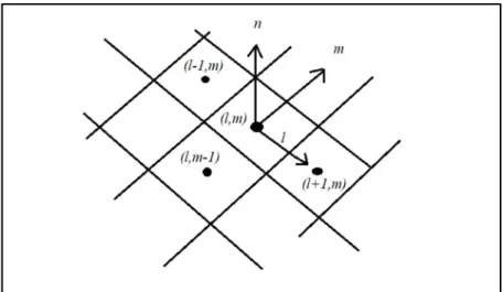
Figure 2.2 Quadrilateral panel (Katz & Plotkin, 2001).
Figure 2.2 shows the panel vertex coordinates (x1, x2, x3, x4, y1, y2, y3, y4, z1, z2, z3, z4), the x, y, z are the coordinates of influenced arbitrary field point P in space. The local frame of reference of the panel is shown.
Consider a wake panel that is shed by an upper panel and a lower panel as shown in the figure (2.3). The equation of the first collocation point where it includes the influence coefficients, source and doublet parameter of each panel can be derived as shown in equation (2.19) (Katz et Plotkin, 2001).
𝐶 𝜇 + ⋯ + 𝐶 𝜇 + ⋯ + 𝐶 𝜇 + ⋯ + 𝐶 𝜇 + 𝐶 𝜇 + 𝐵 𝜎 = 0 (2.19)
Figure 2.3 demonstrates the Kutta-condition on trailing edge. This will add another equation to the panel’s matrix. The Kutta-condition is used to calculate the doublet at the wake panel which will remain constant for the rest of the wake panels decaying away from the trailing edge of the wing. The doublet of the wake panel is the difference between the upper and lower doublet, as shown in equation (2.20).
21
𝜇 = 𝜇 − 𝜇 (2.20)
Figure 2.3 Kutta condition at the trailing edge (Katz & Plotkin, 2001)
The previous equation (2.19) consists of N equations with N+1 unknown, where N is the number of panels. The Kutta-condition is used to add the N+1 equation to the matrix of N equations with N+1 unknowns. Equation (2.19) will transform into equation (2.21).
𝐶 𝜇 + ⋯ + (𝐶 + 𝐶 )𝜇 + ⋯ + (𝐶 − 𝐶 )𝜇 + ⋯ + 𝐶 𝜇 + 𝐵 𝜎 = 0
(2.21)
The equation (2.21) can be simplified into equation (2.22).
𝐴 𝜇 = − 𝐵 𝜎
(2.22)
Since the wake shedding is not taken into account, then 𝐴 = 𝐶 . In matrix form, equation (2.22) will transform into equation (2.23).
⎝ ⎜ ⎛ 𝑎 𝑎 𝑎 𝑎 𝑎𝑎 ⋯ … … 𝑎 𝑎 𝑎 ⋮ ⋱ ⋮ 𝑎 𝑎 ⋯ 𝑎 ⎠ ⎟ ⎞ ⎝ ⎜ ⎛ 𝜇 𝜇 𝜇 ⋮ 𝜇 ⎠ ⎟ ⎞ = − ⎝ ⎜ ⎛ 𝑏 𝑏 𝑏 𝑏 𝑏 𝑏 ⋯ … … 𝑏 𝑏 𝑏 ⋮ ⋱ ⋮ 𝑏 𝑏 ⋯ 𝑏 ⎠ ⎟ ⎞ ⎝ ⎜ ⎛ 𝜎 𝜎 𝜎 ⋮ 𝜎 ⎠ ⎟ ⎞ (2.23)
This matrix represents a set of N linear equations with N unknown. Note that Ajj =0.5 on the diagonal of the panel except when the panel is at the edge of the trailing edge (Katz & Plotkin,2001). Since the source strength is known (equation 2.17) then we can establish a right-hand side matrix, and this will be shown in the equation (2.24).
⎝ ⎜ ⎛ 𝑎 𝑎 𝑎 𝑎 𝑎𝑎 ⋯ … … 𝑎 𝑎 𝑎 ⋮ ⋱ ⋮ 𝑎 𝑎 ⋯ 𝑎 ⎠ ⎟ ⎞ ⎝ ⎜ ⎛ 𝜇 𝜇 𝜇 ⋮ 𝜇 ⎠ ⎟ ⎞ = ⎝ ⎜ ⎛ 𝑅𝐻𝑆 𝑅𝐻𝑆 𝑅𝐻𝑆 ⋮ 𝑅𝐻𝑆 ⎠ ⎟ ⎞ (2.24)
2.1.5 Computations of surface velocities and pressure
The interest of this method for this study is its ability to compute surface velocities and the velocities everywhere in the flow field, and the parametric aerodynamic coefficients on the solid body. After calculating the strength of the doublet, the potential velocity outside the surface is calculated. There are two perturbation velocity directions: the normal 𝑞 and the tangential 𝑞 , 𝑞 components. These components are shown in the equations (2.25) respectively (Katz & Plotkin, 2001).
𝑞 = 𝜎 𝑞 = −𝜕𝜇 𝜕𝑙 (2.25) 𝑞 = − 𝜕𝜇 𝜕𝑚
23
Figure 2.4 Panel local coordinate system to evaluate the tangential velocity components
The velocity component in l direction, equation (2.26).
𝑞 = 1
2∆𝑙(𝜇 − 𝜇 )
(2.26)
where ∆𝑙, is the panel length in the l direction. The total velocity at a collocation point N is the summation of the free stream velocity and the perturbation velocity, equation (2.27).
𝑄 = (𝑄 , 𝑄 𝑄 ) + (𝑞 , 𝑞 , 𝑞 ) (2.27)
The pressure coefficient for each panel is calculated by equation (2.28).
𝐶 = 1 − 𝑄 𝑄
(2.28)
Equation (2.28) calculates the aerodynamic pressure coefficient on one panel. The total aerodynamic load is calculated by adding all aerodynamic loads for each panel together.
2.1.6 Velocity calculations in the farfield
With the known source and doublet element at each panel from the previous calculations, Katz et Plotkin (2001) identified a way to calculate the velocity at an arbitrary point in the farfield.. The source and doublet at each panel influence the velocity in the near field. Thus, the velocity of the arbitrary point P (x, y, z) could be calculated from the velocity potential, when the distance is about 3-5 times larger than the panel size, as follow (Katz & Plotkin, 2001).
Φs( , , ) = −𝜎𝐴 4𝜋 (𝑥 − 𝑥 ) + (𝑦 − 𝑦 ) + (𝑧 − 𝑧 ) (2.29) Φd( , , ) = −𝜇𝐴𝑧 4𝜋. (𝑥 − 𝑥 ) + (𝑦 − 𝑦 ) + (𝑧 − 𝑧 )
With Φs and Φd are the potential flow due to source and doublet respectively, 𝜎 is the source element, 𝜇 is the doublet element, A is the panel area, (x, y, z) are the coordinate of the point of interest P in the farfield, (x0, y0, z0) are the collocation point coordinate of the panel (z0 = 0). Equation (2.29) applies when the distance is 3-5 times bigger than the panel diameter. Bear in mind that this equation is set up for one panel. Since the wing possesses more than one panel then the summation of those influenced velocities at the point P will be considered. On the wing surface, the velocities are known but in the farfield, the velocity components based on the source element are calculated with equation (2.30) (Katz & Plotkin, 2001).
𝑢 (𝑥, 𝑦, 𝑧) = 𝜎𝐴(𝑥 − 𝑥 ) 4𝜋 (𝑥 − 𝑥 ) + (𝑦 − 𝑦 ) +𝑧 𝑣 (𝑥, 𝑦, 𝑧) = 𝜎𝐴(𝑦 − 𝑦 ) 4𝜋[(𝑥 − 𝑥 ) + (𝑦 − 𝑦 ) +𝑧 ] (2.30) 𝑤 (𝑥, 𝑦, 𝑧) = 𝜎𝐴(𝑧 − 𝑧 ) 4𝜋[(𝑥 − 𝑥 ) + (𝑦 − 𝑦 ) +𝑧 ]
25
(𝑢 , 𝑣 , 𝑤 ) are the coordinates of the velocity potential due to source, (x0, y0, z0) are the collocation point coordinates for each panel and A is the panel area. In the farfield, the velocity components based on the doublet element are, (Katz & Plotkin, 2001) equation (2.31).
𝑢 (𝑥, 𝑦, 𝑧) = 3𝜇𝐴(𝑥 − 𝑥 )𝑧 4𝜋[(𝑥 − 𝑥 ) + (𝑦 − 𝑦 ) +𝑧 ] 𝑣 (𝑥, 𝑦, 𝑧) = 3𝜇𝐴(𝑦 − 𝑦 )𝑧 4𝜋[(𝑥 − 𝑥 ) + (𝑦 − 𝑦 ) +𝑧 ] (2.31) 𝑤 (𝑥, 𝑦, 𝑧) = − 𝜇𝐴[(𝑥 − 𝑥 ) + (𝑦 − 𝑦 ) −2𝑧 ] 4𝜋[(𝑥 − 𝑥 ) + (𝑦 − 𝑦 ) +𝑧 ]
The velocity components due to the doublet element (𝑢 , 𝑣 , 𝑤 ) are obtained by differentiating the equation (2.29) with respect to (x, y, z) respectively. Then, those three velocity components (due to source and doublet) will be subtracted from the flow velocity components to form the fluid velocity (Ashby et al., 1991), equation (2.32).
𝑈 (𝑥, 𝑦, 𝑧) = 𝑈𝑡 − 𝑢 (𝑥, 𝑦, 𝑧) − 𝑢 (𝑥, 𝑦, 𝑧)
𝑉 (𝑥, 𝑦, 𝑧) = 𝑉𝑡 − 𝑣 (𝑥, 𝑦, 𝑧) − 𝑣 (𝑥, 𝑦, 𝑧) (2.32) 𝑊 (𝑥, 𝑦, 𝑧) = 𝑊𝑡 − 𝑤 (𝑥, 𝑦, 𝑧) − 𝑤 (𝑥, 𝑦, 𝑧)
Ut, Vt and Wt are the free stream velocity components in (x, y, z) direction respectively which
are respectively equal to Q components with respect to the global frame of reference.
2.1.7 Closing the wing tip
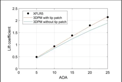
The mesh generated by the 3DPM program available in the annexes of the book by Katz et Plotkin (2001) has an open wing tip. A wing with an open wing tip generates a lift force coefficient that is not linear with respect to the angle of attack. To solve this problem a correction is made to the book program such as to close the wing tip. The aim is to correct the
flow around the wing tip. Since the flow solution depends on the calculations of the parameters at each panel, then a correction of the flow at the tip will affect the whole solution. Next figures 2.5 and 2.7 shows the geometry generated by the 3DPM code before and after closing the wing tip.
Figure 2.5 shows how the program creates a wing from IB+1 airfoil coordinates, which is read from a file. Note that IB+1 is the number of the coordinates of the airfoil. The x and z coordinates are given in anticlockwise order around the airfoil, with a duplicated node at wing tip. Thus, the coordinates of node 1 should be the same as coordinates of node IB+1.
27
Figure 2.6 Strategy for closing the wing tip by adding some panels.
Figure 2.6 presents the airfoil at the tip section. The panels are quadrilateral. The counter I stands for the X direction while J is for Y direction. The coordinates of the wing are represented as from 1 to IB+1. The wing spanwise sections are represented from 1 to JB+1 starting from the root section along the tip. This step enables to create corner points on the airfoil creating the corner stones of the panels. In addition, based on the corner point calculation, the collocation points, which are located in the center of each panel are created. Two specific points should be mentioned: at the trailing edge and at the leading edge. At the trailing edge and leading edge, the panel points are superposed. The first and last point of the counter are also separated. In this case, the program will treat the panel as quadrilateral with a size of length 0, and not triangular. It is necessary to mention that the strength and doublet formulation allow a length of 0. The wing tip closure will correct slightly the flow and affect the pressure and lift coefficients.
Figure 2.7 Wing after closing the wingtip.
The figure 2.7 shows the wing with closed wingtip, with the QF node coordinate at span position J=JB+1=JB1. The corner points coordinates are stored in QF (I, J, 1-3) from I=1 to I=IB+1=IB1. To close the tip, nodes should be added along the camber line such that the wing tip panels can be created. These node coordinates will be stored in QF at J=JB+2=JB2. The new coordinates are obtained by taking the middle position between upper nodes and lower nodes. It is thus necessary to have the same number of nodes on the upper side and the lower side of the airfoil. As mentioned, the panels consist of corner points and collocation points. Let’s consider that the coordinates of the airfoil at the wing tip are called as (Xt, Yt, Zt), where
t tends to tip section and n tends to the number of airfoil coordinates. So, the additional corner
points could be found by the summation of the top point of the airfoil coordinate plus the lower point divided by two. Thus, at the tip, the corner points are calculated as follows, equation (2.33). 𝑋 ( , ,… ) = 𝑋 ( , , ... )+ 𝑋 ( ,( ),( ) ... ) 2 𝑌 ( , ,… )=𝑌 ( , , ... )+ 𝑌 ( ,( ),( ) ... ) 2 (2.33) 𝑍 ( , ,… )= 𝑍( , , , ... )+ 𝑍 ( ,( ),( ) ... ) 2
29
where (𝑋 , 𝑌 , 𝑍 ) is the new coordinates of the tip panel corner points, and (𝑋 , 𝑌 , 𝑍 ) are the corner points coordinates at the wing tip section. The collocation point is at the center of the panel, calculated by the equation (2.34).
𝑋 ( , , ,…, ) =𝑋 ( , , ,…, )+ 𝑋 ( , , … )+ 𝑋( , , ,…, )+ 𝑋( , , ,… ) 4 𝑌 ( , , ,…, ) = 𝑌 ( , , ,…, )+ 𝑌 ( , , … )+ 𝑌( , , ,…, )+ 𝑌( , , ,… ) 4 (2.34) 𝑍 ( , , ,…, ) =𝑍 ( , , ,…, )+ 𝑍 ( , , … )+ 𝑍( , , ,…, )+ 𝑍 ( , , ,… ) 4
where, (𝑋 , 𝑌 , 𝑍 ) are the new collocation points coordinates of the tip panels. Note that after adding the tip panels, the parameters like doublet and source are also calculated and added to the wing surface panels using the equation (2.24) mentioned before in section 2.1.
2.2 Trajectories simulations
In the previous section (2.1), the 3DPM provided all the necessary parameters and flow field information for the problem. Now in this section, a trajectory computation strategy will be held. Before presenting the trajectory calculation model, the definitions for the frame of references are required. A fixed or global frame of reference and local frame of reference for the particle are represented respectively as (X, Y, Z) and (Xp, Yp, Zp). The velocities are divided into two: the velocity of the particle in the global frame of reference noted as (Up, Vp, Wp), and the velocity of the fluid (air) in the global frame of reference noted as (𝑈 , 𝑉 , 𝑊 ) calculated in section 2.1 equation (2.32). The relative velocity 𝑽 = [𝑈𝑟; 𝑉𝑟; 𝑊𝑟] of the particle in the global frame of reference is calculated as following, equation (2.35).
𝑈 = 𝑈 − 𝑈𝑝
𝑉 = 𝑉 − 𝑉𝑝 (2.35)
To calculate the trajectory of the particle in space, the Newton’s second law of motion is applied to the particle, equation (2.36). An illustration of the forces applied to the particle is shown in figure 2.8.
𝐹⃗ = 𝑚𝑎⃗ (2.36)
Figure 2.8 Forces applied to the particle with respect to the relative wind velocity
The figure 2.8 represents the ice particle characteristics. L is the length, l is the width and e is the thickness of the particle. The local and the global frame of reference are also shown. The aerodynamic forces as well as the wind direction are illustrated. To integrate the equation of motion with respect to the global frame of reference axis, the equation (2.36) will transform into equation (2.37). 𝐹𝑥 = 𝑚𝑑𝑈 𝑑𝑡 𝐹𝑦 = 𝑚𝑑𝑉 𝑑𝑡 (2.37) 𝐹𝑧 = 𝑚𝑑𝑊 𝑑𝑡 − 𝑚𝑔 This expression involves the following terms:
• 𝐹𝑥, 𝐹𝑦, 𝐹𝑧 are the projections of the forces in the x, y, and z axis (N). • m is the mass of the particle (kg).
31
The position of the particle is determined by integrating two times the acceleration of the particle with respect to time. The positions of the particle at each time step construct the particle path. While moving, the particle rotates in different directions with respect to the three local main axis. The orientation of the particle is defined by three angles called Euler’s angles: rolling, pitching and yawing moment are associated to Φ, θ and Ψ which are the angles of rotation around Xp, Yp and Zp respectively. The moments applied to the particle are the
pitching, yawing, and rolling moment. The equation of moment is represented by the following, equation (2.38) (Ignatowicz et al., 2019).
𝐼 𝑄𝑃 𝑅 = 𝑴𝒕− 𝑄𝑃 𝑅 × 𝐼 𝑄𝑃 𝑅 (2.38)
This expression involves the following terms: • I is matrix of inertia (kg.m2).
• 𝜴 = 𝑄𝑃
𝑅 the angular velocity of the local frame of reference (rad/s). • 𝑴𝒕 the total moment of the particle of the local frame of reference (N.m).
• × is the cross product operator.
To calculate the aerodynamic forces at each time step is a complex task to do. That’s why a simplified solution is provided by Richards, Williams, Laing, McCarty, et Pond (2008). They claim to reduce the forces computation time and introduce a new resultant normal aerodynamic force Fnp directed perpendicular to the flat plate in the positive direction of the z-axis from the center of pressure of the particle. The resultant normal force is expressed by equation (2.39).
𝐹 = 0.5𝜌|𝑽𝒓𝒆| 𝐿𝑙𝐶 (2.39)
The parameters of this equation are as follows: • 𝜌 is the density of the air (kg/m3).
• 𝑽𝒓𝒆 is the relative velocity in the local frame of reference (m/s).
• 𝐶 is the normal resultant force coefficient.
• 𝐿 and 𝑙 are the length and width of the flat plate (m).
Figure 2.9 depicts the particle motion. The two frames of references are shown: the general frame of reference and the particle local frame of reference. The center of gravity lies at the same point as the geometrical center of the particle because the particle is assumed to be a rectangular homogenous flat plate. The center of pressure shown in the picture is not the real fixed point but to show that most of the time the center of gravity and the center of pressure are not at the same point.
Figure 2.9 Motion of the flat plate representation
The normal force coefficient is found through experiments by Richards et al. (2008). Richards has been working to find out that the normal force coefficient depends on the side slip angle β and the angle of attack α. The angle of attack and the side slip angle is calculated as follows in equation (2.40) and presented in figure 2.8 (Richards et al., 2008).
33
𝛼 = 𝑎𝑟𝑐𝑠𝑖𝑛 𝑊
|𝑽𝒓𝒆| (2.40)
𝛽 = 𝑎𝑟𝑐𝑠𝑖𝑛 𝑉
|𝑽𝒓𝒆|cos (𝛼)
Richards et al. (2008) founds also that the normal force coefficient also depends on the surface ratio of the flat plate. The surface ratio of the flat plate is defined to be the length over the width of the same flat plate. By adjusting the surface ratio of the flat plate and calculating the angle of attack and side slip angle, the CN is finally found by interpolation through these
correlations. Once the force is expressed in the local frame of reference of the plate, Fnp is then
being transformed to the general frame of reference and thus equation (2.39) is solved.
The classic transformation of the vector force from local particle frame of reference to the global frame of reference is done through Euler’s transformation. This transformation is done through a transformation matrix we called it 𝑅 (𝑞). For instance, the transformation of the velocity vector is done by the equation (2.41). This transformation is done using Euler’s angles.
𝑽𝒓𝒆= 𝑅 (𝑞)𝑽𝒈 (2.41) 𝑽𝒈= 𝑅 (𝑞) 𝑽𝒓𝒆 𝑅 (𝑞) = 𝑞 + 𝑞 − 𝑞 −𝑞 2𝑞 𝑞 + 2𝑞 𝑞 2𝑞 𝑞 − 2𝑞 𝑞 2𝑞 𝑞 − 2𝑞 𝑞 𝑞 − 𝑞 + 𝑞 −𝑞 2𝑞 𝑞 + 2𝑞 𝑞 2𝑞 𝑞 + 2𝑞 𝑞 2𝑞 𝑞 − 2𝑞 𝑞 𝑞 − 𝑞 − 𝑞 +𝑞 (2.42)
𝑽𝒈 is the velocity vector in the local frame of reference of the particle. 𝑅 (𝑞) is a matrix which depends on the quaternions calculated in equation (2.43). The quaternions will model the rotation of the particle around a single axis which is directed by a unit vector. The quaternions are four scalar expressions that depends on Euler’s angles which characterize the orientation of the particle at every rotation (Fu, Huang, & Gu, 2013) (Diebel, 2006). These relations are expressed by the equation (2.43).
𝑞 = cos 𝛷 2 cos 𝜃 2 cos 𝛹 2 + sin 𝛷 2 sin 𝜃 2 sin 𝛹 2 (2.43) 𝑞 = cos 𝛷 2 sin 𝜃 2 sin 𝛹 2 − sin 𝛷 2 cos 𝜃 2 cos 𝛹 2 𝑞 = − cos 𝛷 2 sin 𝜃 2 cos 𝛹 2 − sin 𝛷 2 cos 𝜃 2 sin 𝛹 2 𝑞 = sin 𝛷 2 sin 𝜃 2 cos 𝛹 2 − cos 𝛷 2 cos 𝜃 2 sin 𝛹 2
The aerodynamic forces pass through the center of pressure. To solve the moment equation (2.38) the direction of the normal force and the center of pressure should be known. After (Richards et al., 2008) the center pressure coordinates are calculated in the equation (2.44).
𝑋 = 𝑐 4 90 − |𝛼| 90 cos(𝜁) (2.44) 𝑋 = 𝑐 4 90 − |𝛼| 90 sin(𝜁)
where c is defined as the chord of the flat plate while 𝜁 is the angle formed between the velocity and local x-axis of the plate Xp. After Richard et al. (2008) the expressions c and 𝜁 are calculated in the equation (2.45).
tan 𝜁 = tan 𝛽𝐿 𝑙
𝑐 = 𝐿𝑙
𝐿|cos 𝛽| + 𝑙|sin 𝛽|
(2.45)
While the particle displaces in the space, it rotates. This rotation is caused by a moment. The moment applied to the particle is divided into two: the static moment and the dynamic moment. The summation of both static and dynamic moment gives the total moment in equation (2.46).
35
The static moment is introduced due to the shifting of the center of gravity from the center of pressure in most cases in the study like shown in figure 2.9. Thus, the static moment Mp is
calculated in the equation (2.47) (Ignatowicz et al., 2019).
𝑴𝒑 = 𝐶 𝐶⃗ × 𝑭 (2.47)
F is the normal aerodynamic resultant force in the global frame of reference, Cp is the center
of pressure and CG center of gravity of the particle. The dynamic moment of the particle is due to the rotation of the particle in the space around the three axis Xp, Yp and Zp. The dynamic moment used, follows the one suggested by Ignatowicz et al. (2019) and calculated in the equation (2.48). 𝑀 =1 2𝜌|𝑉 | 𝑙 𝐿𝐶 𝐿 𝑙𝐶 0 (2.48)
In the equation (2.48), 𝐶 , 𝐶 and 𝐶 stands for the dynamic moment coefficient components. The dynamic moment coefficient is calculated by the following equation (2.49) (Ignatowicz et al., 2019). 𝐶 = ⎣ ⎢ ⎢ ⎢ ⎢ ⎡𝑠𝑖𝑔𝑛(𝑃)𝐹 |𝑃| 𝑃 𝑠𝑖𝑔𝑛(𝑄)𝐹 |𝑄| 𝑄 0 ⎦ ⎥ ⎥ ⎥ ⎥ ⎤ (2.49)
where the expressions for P0 and Q0 stands for maximum angular velocity and it is calculated by the following equations (2.50) (Ignatowicz et al., 2019).
𝑃 = 2(−1.25𝑒 𝑙+ 0.516) |𝑉 | 𝑙 (2.50) 𝑄 = 0.8|𝑉 | 𝐿