HAL Id: hal-02056716
https://hal-mines-albi.archives-ouvertes.fr/hal-02056716
Submitted on 5 Mar 2019
HAL is a multi-disciplinary open access
archive for the deposit and dissemination of sci-entific research documents, whether they are pub-lished or not. The documents may come from teaching and research institutions in France or abroad, or from public or private research centers.
L’archive ouverte pluridisciplinaire HAL, est destinée au dépôt et à la diffusion de documents scientifiques de niveau recherche, publiés ou non, émanant des établissements d’enseignement et de recherche français ou étrangers, des laboratoires publics ou privés.
Optimization of coat-hanger melt distributors for the
wire coating process
Nadhir Lebaal, Fabrice Schmidt, Stephan Puissant, Daniel Schläfli
To cite this version:
Nadhir Lebaal, Fabrice Schmidt, Stephan Puissant, Daniel Schläfli. Optimization of coat-hanger melt distributors for the wire coating process. Proceedings of the Polymer Processing Society, Jun 2008, Salerno, Italy. �hal-02056716�
OPTIMIZATION OF COAT-HANGER MELT DISTRIBUTORS FOR THE
WIRE COATING PROCESS
N. Lebaal1, F.M. Schmidt2*, S. Puissant1 and D. Schläfli 3
1
Institut Supérieur d’Ingénierie de la Conception (GIP-InSIC), 27 rue d’Hellieule, 88100 Saint-Dié-des-Vosges, France - [email protected]; [email protected]
2
Ecole des mines d’Albi Carmaux (ENSTIMAC) , Centre de Recherche Outillages, Matériaux et Procédés «CROMeP», Campus Jarlard- Route de Teillet 81013 Albi Cedex 9, France - [email protected]
3
Extrusion Maillefer SA Route du bois 37 - Ecublens – Switzerland - [email protected]
Abstract
The objective of the rheological design of extrusion dies in the wire coating process is to distribute the melt around the conductor uniformly. If the manifold is not designed properly, the velocity at the die exit may be not uniform.
However, in this paper we present an optimal design approach, this approach involves coupling an optimization routine with mesh generators and three-dimensional finite element simulation software. The objective is to obtain optimal coat-hanger melt distributor geometry to ensuring a homogeneous exit velocities distribution without increase the pressure at the die entrance. For this purpose, we investigate the effect of the design variables in the objective and constraint function by using Taguchi method. In the second study we use the global response surface method and SQP algorithm in order to improve the exit velocities distribution by modify the manifold geometry using a simplified design model.
1. Introduction:
The design of dies for polymer extrusion often involves trial and error corrections of the die geometry to achieve uniform flow at the exit. However manual correction to die geometry is a time consuming and costly procedure. CHEN et al. [1] showed using Taguchi method that, the operating conditions, the materials change and the die geometry have a great influence on the velocities distribution at the die exit. Wang et al. [2] investigate the effect of manifold angle and the contour of the manifold cross section on the flow distribution in the coat-hanger die using a three-dimensional finite element code with isothermal flow of power low fluids.
Winter and Fritz [3] presented a theory for the design of coat-hanger dies, with circular or rectangular section of the distribution manifolds. For the latter, provided a height aspect ratio of the manifold, the theory predicts material independence of the flow distribution. However, uniform distribution may not be achieved in practice.
Considerable gains are to be expected from the use of adequate computational tools, for the numerical prediction of polymer melt flows through extrusion dies [4-6]. Nevertheless these computational tools are usually not user-friendly and require large CPU times. However, obtaining the optimum parameters is often the result of a tiresome work of trial and error corrections, during which, the various numerical solutions are tested and modified.
The die complexity, the nonlinear relationship of the rheological behaviour complicate the design of die for
polymer extrusion; further increases the difficulty of the die optimization problem and leading by this fact to a high number of numerical tests while the CPU time is often very high for three-dimensional simulations. Nevertheless, if the research of the quality criterion is made without specific methodology, it can easily lead to a solution which will not be optimal.
The global automatic optimization of extrusion die design still remains a challenge and it is the purpose of this work to contribute to further developments of automatic die design tools. It was the need to have a design process less dependent on personal knowledge. This is also the main purpose of a die design code that is currently being developed, which main objective is to carry out the automatic search of the optimal flow channel geometry.
The code consists of an optimization routine coupled with geometry and mesh generators and 3D computational software [7], based on the finite element method able to predict, the complex 3D flow and the temperature distribution. Because the quality criteria (objective and constraint functions) are implicit compared to the optimization parameters and their evaluations need a complete numerical analysis of the extrusion process, which requires a large computation times; the Response Surface Method [8-9] (RSM) is adopted and coupled with an auto adaptive strategy of the research space to obtain the optimum parameters with low cost (acceptable computation times), and with a good accuracy.
2.Experimental data:
2.1 Die design:
The objective of this study is to find a design procedure for a distribution system that gives better uniformity of flow, i.e. uniform exit velocity and uniform average residence time over the die width. This uniformity should preferably be achieved with a die geometry that is independent of flow rate or polymer viscosity. Winter and Fritz [3] present a theory based on simplified flow model for the design of rectangular manifold to obtain a homogeneous exit velocity distribution.
Given the polymer flow properties, the width of distribution system, 2b, the height of the slit h, and the volume flow rate
Q
v=
2
bh
v
s we can calculate the corresponding manifold contour lines y(x) as follows :C x g x g x g x g Bb x y + ⎥ ⎥ ⎦ ⎤ ⎢ ⎢ ⎣ ⎡ + + − + − + = 1 ) ( 1 1 ) ( 1 ln 2 1 ) ( ) ( 1 2 3 ) ( (1) with a function
(
)
[
2]
1 1 ) ( ) (x = H x h − − g (2)The integration constant is equal to zero, C=0, given by the choice H(x)=h at y=0.
The dimensionless parameter of the solution is defined as b f h a B= p (3)
For a manifold of constant aspect ratio, a=W/H, the manifold has the side faces
( )
[
(
)
(
)
]
13 h f a x b h x H = − p (4)(
)
[
2 2]
13 ) ( ) (x aH x ha h b x fp W = = − (5) Figure 1. Sketch of coat hanger distribution system with wide manifold and narrow slit flow region. For a manifold of constant width W>>H, the diedesign is materials independent. The thickness variation of the manifold is then given by:
( )
x h(
b x)
WH = − (6)
The corresponding contour lines y(x) is given as follows :
( )
x =2W(
b−x)
W−1y (7)
In order to verify the design procedure, initial distributor is built according to the theory (eq.6-7) presented in [3] and tested. This coat hanger melt distributor has a diameter of 106 mm and a slit height of 3 mm, with a flat manifold of constant width W=50 mm. The initial manifold height is a little bit more than
twice the slit height. Because of the high aspect ratio, the sidewall effects on the flow are small and almost independent of material changes. Therefore, the flat and wide manifold should result in a long (194 mm), but material insensitive distributor.
2.2 Materials:
A low density polyethylene (LDPE) referred Lupolen 1812D is selected for this example.
A Carreau Yasuda/Arrhenius viscosity model is used to characterize the temperature and shear rate dependence of viscosity: ( ) a m a s 1 0 0 1 − ⎥ ⎥ ⎦ ⎤ ⎢ ⎢ ⎣ ⎡ ⎟⎟ ⎠ ⎞ ⎜⎜ ⎝ ⎛ + = τ γ η η η & (9) with ⎥ ⎥ ⎦ ⎤ ⎢ ⎢ ⎣ ⎡ ⎟ ⎟ ⎠ ⎞ ⎜ ⎜ ⎝ ⎛ − = ref ref T T T T) ( )exp 1 1 ( 0 0 η β η (10)
The rheological properties (Tab. 1) are obtained by the data bases of Rem3D® (MatDB®).
Table 1. Rheological parameters. Material LDPE 0 η [Pa.sm] m a
τ
s [Pa] Tref [K]β
[K] 1812D 202278 0,35 1 10555 423 61563. Experimental measurements and numerical validation:
3.1 Experimental measurements:
The experimental measurements are established for LDPE Lupolen 1812D [10]. At the exit of the distributor, a flow separator divides the flow into 8 strips. The melt distribution is established by the measurement of the mass flow rate at some 36 seconds periods for each partial flow. It should be noted that a length of tools of 30 mm is used after the manifold length. Since the die and tools will have a more significant resistance to the flow, which will make it possible to improve the exit velocity distribution. By symmetry, the measurements of flow rate on sectors 1 and 5 remain unchanged. On the other hand, for sectors 2, 3, and 4 we respectively take the average of the measurements of flow established for the sectors (2 and 8); (3 and 7); (4 and 6).
3.2 Numerical simulations:
The numerical simulations were carried out under Rem3D®. Due the symmetry, we model only half of the die cavity where the finite element model includes 51512 nodes and 252593 elements. The process parameters (Q ,v
T
wandTm
), are referred to in table 2Table 2. Process parameters Flow rate Q v [mm3/s] Die wall temperature (
T
w) [°C] Melt temperature (Tm
) [°C] 47738 194 193 For each sector, the dimensionless average velocity is defined by:v
v
v
s i a i=
(12) with:∑
==
s N j s j s s iv
N
v
11
(13) wherev
and s iv
are respectively the global average velocity and the average velocity for each sector, sj
v
is the velocity in each node
j
which belongs to the sectorsS
i and sN
is the number of node for each sector on the die exit.The global relative deviation s g
E
is calculated by the sum of the relative deviations in each sector as follows:∑
∑
= =−
=
=
Ns i a i Ns i s i s gE
v
E
1 11
.
100
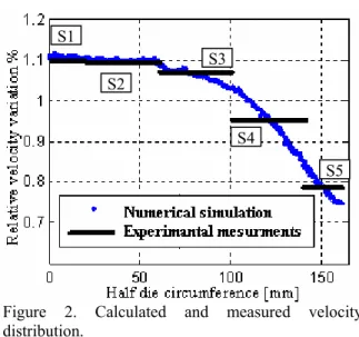
(14)Table 3 indicates the measured and calculated dimensionless average velocities using Rem3D® software for each sector at the die exit.
Table 3. Results of Experimental measurements and numerical simulations:
Tests 1
Materials LDPE Lupolène1812D Average velocities a
v
exp a calv
1S
1,098 1.101 2S
1,094 1.101 3S
1,071 1.059 4S
0,952 0.950 5S
0,785 0.789 s gE
52.6 52.23Figure 2 illustrates the measured and calculated exit velocity distribution for the initial die design. The manifold of this initial die is of constant width and has an initial aspect ratio of h/w=0.11. According to the theory presented in [3], this design should be practically material-independent. However, distribution non-uniformity is important and perfectly predicted by the calculation (Figure 2). The velocity is more important in the sectors (1, 2, and 3) and weaker in the sections (4, and 5).
However, the observed non uniform velocity distribution are not predicted by the theory; it is due to the already mentioned three-dimensional character of the manifold flow. Clearly, 3-D effects are important for such designs, but they are beyond the scope of the design theory.
Figure 2. Calculated and measured velocity distribution.
After these validation, the optimization procedure is introduced in order to improve the exit velocity distribution by modify the manifold geometry.
4. Optimization problem
4.1 Objective and constraint functions:
This optimization problem consists in determining an optimal geometry to homogenize the exit velocity distribution, which corresponds to the minimum of the objective function (
J
). While preventing that the pressure "pressure loss" increases more than the pressure obtained by the initial geometry; this condition is translated by a constraint function (g
).⎪ ⎪ ⎩ ⎪⎪ ⎨ ⎧ ≤ − = = Φ 0 ) ( ) ( ) ( min 0 0 0 P P P g that Such E E J (15)
where E is the velocity deviation , is defined as follows: ⎟ ⎟ ⎠ ⎞ ⎜ ⎜ ⎝ ⎛ ⎟⎟ ⎠ ⎞ ⎜⎜ ⎝ ⎛ − =
∑
N= i i v v v N E 1 1 (16)where
P
0 andE
0 are respectively the pressure and velocity deviation in the initial die, N is the total nodes number at the die exit in the mid plane,v
i is the exit velocity, andv
is the average exit velocity, is defined as:∑
= = N i i v N v 1 1 (17)The constraint function (
g
) is selected in a way to be negative if the pressure is lower than the pressure obtained by the initial die design (the pressure must be even lower compared to the initial pressure).4.2 Optimization variables
For a diameter of 106 mm (b=166.5mm), and a slit height of 3 mm and initial manifold of constant width,
S1 S2
S3
S4
the contour lines y(x) and the thickness variation of the manifold are calculated starting from equations (6-7) given by Winter and Fritz [3]. During the optimization procedure, two variables witch represent the aspect ratio, a=W/H, and the shape factor, f , will be p
optimized in order to ensure better exit velocity distribution. The new manifold contour lines y(x) and manifold thickness H(x) are calculated starting from equations (1-5).
Initially, the manifold width W0 =50mm is constant,
and the shape factor fp is unity. During optimisation;
the aspect ratio a=W/H and the shape factor f can p
vary respectively between: 0.5≤ k≤10
a and0≤ k ≤1
p
f
4.3 Sensitive analyses:
A Taguchi’s design of experiments method [11] is used to investigate the sensitive analysis of the design variables. A central composite design of experiment (CCD) [11], is used to calculated the effect of each variable over all the field of research by studying the contribution of each variable on the responses variation “objective and constraint functions ". The CCD gives 5 levels per variable. The various levels are represented from 1 to 5 respectively giving the values of the minimum to the maximum of each variable.
a1 a2 a3 a4 a5 fp1 fp2 fp3 fp4 fp5 -20 -10 0 10 20
Factor (variable) level
A v e ra ge ef fe c t o n t h e obj ec ti v e f u n c ti o n Variable a Variable fp Mean value
Figure 3. Effect of factor levels on the objective functions. a1 a2 a3 a4 a5 fp1 fp2 fp3 fp4 fp5 -4 -2 0 2 4 6 8
Factor (variable) level
A v e rag e ef fe c t on t h e pr e s s u re Variable a Variable fp Mean value
Figure 4. Effect of factor levels on the constraint functions.
The graphical representations of factors effect at different levels are shown in Fig. 3-4. We note that the both variables (manifold aspect ratio "a" and shape factor " fp ") have more effect on the objective function and on the pressure. The optimum parameter level for minimum value of objective and constraint (pressure) functions are respectively a4 fp 4 and a2
fp(1-2).
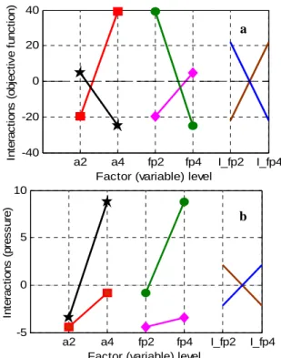
In order to study the interactions between the two variables the graphical representations of factors interactions at different levels are shown in Fig. 5 (a and b). a2 a4 fp2 fp4 I_fp2 I_fp4 -40 -20 0 20 40
Factor (variable) level
In te ra c ti o n s ( o b je c ti v e fu n c ti o n ) a2 a4 fp2 fp4 I_fp2 I_fp4 -5 0 5 10
Factor (variable) level
In te ra c ti o n s (p re s s u re )
Figure 5. Interactions of factor levels on the objective (a) and constraint (b) functions.
This figure represent the interactions between the two variables, by the average response with a, then fp in
X-coordinate and by the value of their interaction, for the both functions (velocity distribution (Fig.5-a) and pressure(Fig. 5-b)). We notes from this figure, that the effect on the objective and constraint function of the variable
a
is very strongly depends on the levels taken by the variable fp and reciprocally, witch implies that the interactions between the two variables is very strong. This strong interaction implies the non-linearity of the objective function.4.4 Optimization procedure:
The RSM consists in the construction of an approximate expression of objective and constraint function starting from a limited number of evaluations of the real function. In order to obtain a good approximation, we used a Kriging interpolation [12-13]. In this method, the approximation is computed by using the evaluation points by composite design of experiments. The Sequential Quadratic Programming
b a
(SQP) algorithm is used to obtain the optimal approximate solution which respects the imposed nonlinear constraints. After that, successive local approximations are built, in the vicinity of the optima by taking into account the weight function of Gaussian type. The iterative procedure stops when the successive optimum of the approximate function are superposed with a tolerance ε=10-6. Finally, another evaluation is
carried out to obtain the real response in the optimization iteration.
An adaptive strategy of the search space is applied to allow the location of the global optimum. During the progression of the procedure, the region of interest moves and zooms on each optimum.
An enrichment of the interpolation is made by recovering responses already calculated, and which are located in the new search space. The iterative procedure stops when the successive points are superposed with a tolerance ε=10-3.
5. Optimization result and Discussion
A study of the effects and interaction of the optimization variables, show that the interaction between the optimization variables is more important. This, indicates that the non linearity of the function to be minimized is more important. The optimization example was carried out for LDPE 1812D and with a flow rate of 120 kg/h. By symmetry, only one half die is modelled.
The optimization results are carried out on a machine Pentium D, 3.4 GHz, 3 Go RAM.
Table. 4. A summary of the optimization results Optimization results Initial die Optimal
die
CPU time 18h40
Iterations 0 2
Objective function
f
1 0.07 Improvement of the velocitydistribution - 93%
Constraint function P/P0 0.98 0.44 Variable a 0.11 1.52
Variable fp 1 0.36
A summary of the optimization results is referred in table 4. According to this table, we note an improvement of the objective function compared to the initial design of 93%. Furthermore, the constraint imposed on the pressure makes it possible to limit the increase in the pressure in the optimal die. We note that the constraint is respected and that the pressure decreased by 56 %. This is do the height manifold thickness.
The optimum solution is reached after two actualization of the research space. The two approximate objective functions are presented respectively in figure 6-7. -1 0 1 -1 0 1 -20 0 20 40 60 80 Variable a Variable fp O b je c ti v e f unc ti on
Figure 6. Approximate objective function (1st research
space) -1 0 1 -1 0 1 -20 0 20 40 60 80 Variable a Variable fp O b jec tiv e f u n c ti o n
Figure 7. Approximate objective function (2ndresearch
space) 0 1 2 3 4 5 6 7 8 9 -10 0 10 20 30 40 SQP iterations A ppr ox im at e obj ec ti v e f u nc ti o n Local optimum Global optimum Local optimum Golobal optimum
Figure 8. Convergence history of the objective function (1stresearch space).
The convergence history during the optimization run using SQP algorithm are shown for both approximations (1st and 2nd research space)
respectively in figure 8 and figure 9. To avoid the fact of falling into a local optimum, and to respect the imposed nonlinear constraint, the best approximate solution among those obtained by the various optimizations is chosen.
The true objective function is then reduced by 93% compared to their initial value.
0 1 2 3 4 5 6 7 -20 0 20 40 60 SQP iterations A p p rox im a te ob je c ti v e f u nc ti on Global optimum Local optimum
Figure 9. Convergence history of the objective function (2nd research space)
The calculated distributor performances are shown in fig 10. Differences between the two materials (LDPE) are predicted. However differences are minimal in term of velocity distribution. We noted in the seam figure that, after optimization, the dimensionless velocities distribution for the Lupolen 1812D are about unit for all die circumference (x). This implies a good velocity distribution compared by the initial die. Nevertheless, using the second material (LDPE 22H760) we observe week degradation of performance of a bout 5% in term of velocity distribution. 0 20 40 60 80 100 120 140 160 0.8 0.9 1 1.1
Half die circumference x [mm]
D im ens ionl es s v e lo c it y di s tr ibut io n
Optimal die Lupolen 1812D Optimal die LDPE 22H760 Initial die Lupolen 1812D
Figure 10. Exit velocity (dimensionless) distribution in the initial and optimal die.
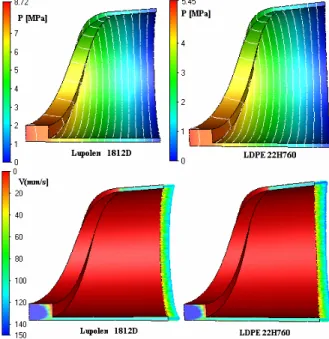
Figure 11. Pressures and exit velocity distribution in initial die design.
Figure 11 presents the exit velocity distributions, and pressures in the initial geometry. The velocity distributions obtained by three-dimensional finite element model show the weakness of the design of one-dimensional model presented by Winter and Fritz [3]. The manifold flow can no longer be treated as a pure 1-D duct flow.
Figure 12. Pressures and exit velocity distribution in optimal die design.
We note in figure 12 that we obtain a good velocity distribution for two polymers. It is noticed that the constraint imposed on pressure is respected since the pressure did not exceed the initial pressure 17 MPa for the seam flow (120Kg/h). The pressure is higher in the case of Lupolene 1812D and it is weaker for the 22H760.
Because of the low aspect ratio, the sidewall effects on the flow are not insignificant and almost no independent of material changes. Therefore, the optimal flat and wide manifold result in a short (80 mm) compared to the initial manifold (193 mm), and the pressure drop decrease of about 50% compared to the pressure obtained by the initial die design (17.1 MPa).
6. Conclusions
The numerical algorithm presented in this work based on the global automatic optimization of extrusion die design shows promise as a tool capable of predicting optimal geometry and to have a design process less dependent on personal knowledge.
The initial die obtained using the theory given by Winter and Fritz [3] gives a non uniform exit velocity distribution due the 3D effect. A comparison between the numerical results and experimental measurements
indicates that the velocity distribution gives a perfect agreement.
To improve the exit velocity distribution an optimization procedure is applied to predict the optimal manifold geometry by means of design model presented in [3]. The optimal 3D die extrusion is a short length compared to the initial die and gives a good exit velocity distribution while minimizing the pressure for the same flow.
7. Acknowledgements
The support of Maillefer SA is gratefully acknowledged.
8. References
1. C. Chen, P. Jen, F. S. Lai, Polym. Eng. Sci. 1997, 37, 188.
2. Y. WANG, Polym. Eng. Sci. 1991, 31, 204. 3. H.H. Winter, H.G.Fritz, Polym. Eng. Sci., 1986,
26, 543.
4. Y. Sun, M. Gupta., Int. Polym. Process., 2003, 18, 356.
5. W.A. Gifford, Polym. Eng. Sci., 2001, 41, 1886. 6. J. M. Nóbrega, O. S. Carneiro, F. T. Pinho, P. J.
Oliveira, Int. Polym. Proces., 2004, 19, 225. 7. L. Silva, PhD Thesis, École Nationale Supérieure
des Mines de Paris, 2004.
8. R. H. Myers, D. C. Montgomery, Response surface methodology, Process and product optimization using designed experiments, second edition, Wiley Inderscience, USA, 2002.
9. N. Lebaal, S. Puissant, F. M. Schmidt, J. Materials
Process. Tech., 2005, 164, 1524.
10. D. Schläfli, Int. Polym. Process., 1995, 10 195. 11. D.C. Montgomery, Design and analysis of
experiments, John wiley & Sons, INC, USA, 2005. 12. N. Lebaal, S. Puissant, F. M. Schmidt, in:
NUMIFORM '07, AIP Conf. Proc. 2007, 908. 13. I. Kaymaz, Struct. Safety, 2005, 27, 133.