Strategic investment and learning with private information
∗Nicolas Klein†and Peter Wagner‡ July 5, 2018
Abstract
We study a two-player game of strategic experimentation in which agents choose the timing of investments which yield uncertain returns over time. Agents learn about future returns through privately observed signals, others’ investment decisions and from public experimentation outcomes when returns are realized. We characterize symmetric equilibria, and we relate the extent of strategic delay of investments in equilibrium to the primitives of the information structure. Agents invest without delay when the most optimistic intermediate belief exceeds a threshold. Otherwise, delay in investments induces a negative learning feed-back which may either escalate or dampen beliefs and investment choices. We highlight how private information in strategic experimentation can increase ex ante welfare because of strategic uncertainty and due to an “encouragement effect of private information”.
1 Introduction
Is transparency good for innovation? The question is at times controversially debated in the public square, often seeming to pit industry executives against regulators.1 We propose a simple model of innovation in which, say, two pharmaceutical companies decide on making an irreversible invest-ment, such as putting a certain medical substance on the market. The quality of the investment option is the same for both companies but initially unknown. Either company has some initial pri-vate information about its quality. As long as the substance is marketed, it generates some positive flow payoff. But, if the substance is of low quality, this will be discovered during its marketing phase after an exponentially distributed time, e.g, because a consumer is harmed. In this case, the drug is banned, the game ends, and the company responsible for causing the harm is fined so heavily that it regrets having marketed the drug.
∗A previous version of this work was circulated under the tile “Learning from strangers.” †Universit´e de Montr´eal and CIREQ, Email: [email protected]
‡University of Bonn, Email: [email protected]
We show that, in our setting, keeping the companies’ initial private information private may be beneficial for welfare.2 Indeed, on account of the irreversibility of investments, agents wait too long before they invest in the hope that the other provides free information. Excessive delay before investments is the result of leadership-aversion. Indeed, the follower can get additional information concerning the quality of the investment by observing the leader’s experience; moreover, conditionally on the project being bad, the leader is more likely to be subjected to the fine. After the first agent has invested, the other agent trades off the forgone returns from investing with the benefit of waiting for more information, without taking into account the positive externality her investment would exert on her partner, leading to a delay in the follower’s investment through a classical free-riding effect.
As our main result shows, not knowing one’s partner’s type may mitigate both sources of inef-ficiency. Indeed, when agents have private information, delaying their investments has drawbacks. An agent can only benefit from waiting to invest if the other agent invests first. However, one agent’s delay may signal bad information to the other, who, in response, may be less willing to invest, thereby reducing the first agent’s incentive to delay. As a result, an agent who received a bad signal may have an incentive to invest without delay nonetheless, in order to encourage the other agent to invest earlier. A second drawback results from each agent’s uncertainty about the other agent’s behavior. For example, an agent who received a good signal may wait in the hope that the other agent invests first. The other agent, however, may have received a bad signal and therefore never invest. Or an agent may delay her investment despite having received a good signal, so as to learn whether or not the other agent invests. However, by delaying her investment, she discourages future investment by the other agent, even if the other has received a good signal. These negative effects of delay under private information can induce agents to invest earlier, and thereby reduce free-riding and leadership aversion. This reduction increases ex-ante social welfare as long as it does not result in inefficient over-investment. For example, an agent with a good signal may invest not knowing the other agent’s signal, but regret investing if she learns that the other agent’s signal is bad. In cases like these, it might be socially desirable to make agents’ private information public. Several papers have investigated the role of private information in games of informational exter-nalities.3 Rosenberg et al.(2013) investigate a game of strategic experimentation with exponential two-armed bandits, where players’ action choices are public information, while the outcomes of these actions are private information. A player’s switch to the safe arm is irreversible. They show that, in their setting, public information is unequivocally good for welfare. Their setup differs from ours inter alia by the fact that their players accrue private information over time, while ours are
2
We do not include consumers in our model. Thus, if we wanted to include them in our welfare calculus, we should have to assume that the fine is set in such a way as to make the firm fully internalize the harm caused.
3
The problem of strategic information acquisition in bandit games has been introduced by Bolton and Harris
(1999) in a Brownian-motion environment. Keller et al.(2005) have extended the analysis to a Poisson setting, while
Keller and Rady(2015) have introduced “bad news” Poisson events. Private information in this setting has also been analyzed inRosenberg et al.(2007).
privately informed at the outset. Furthermore, there are no payoff externalities inRosenberg et al.
(2013), so that, once they have irreversibly exited the game, their players do not care about their partner’s behavior any longer. Our players, by contrast, decide on when irreversibly to enter the market, and thus might have incentives to bias their partner’s entry decision even conditional on their entering themselves.
Heidhues et al.(2015) investigate the problem with public reversible actions and private payoffs, while allowing for cheap-talk communication among players. They show that equilibria with public information can always be replicated under private information, so that private information is unequivocally good for welfare. This conclusion heavily depends on their assumption that players can communicate among each other. In contrast, Bonatti and H¨orner (2011), analyze the case of unobservable and reversible actions and observable outcomes, and find that private information boosts welfare in their setting. The reason is that, with observable actions, a deviation by a player may render the other players more optimistic, and hence more willing to pick up the slack caused by the deviation. This in turn makes deviating more attractive under public information.
In Chamley and Gale (1994) andMurto and V¨alim¨aki (2011, 2013) , information is dispersed throughout society, and agents decide when to take an irreversible action. As in our setting, information is inefficiently aggregated because investors have an incentive to delay their decision so as to acquire more information by observing the behavior of others. The players do not observe the results of their partners’ experimentation directly. Moreover, once an agent takes an action, she effectively exits the game, and is no longer affected by others decisions. In our setting, by contrast, players continue to be affected by others actions after taking their irreversible action, and thus have an incentive to influence their partners actions and beliefs when making their irreversible investment decision.
A closely related paper is D´ecamps and Mariotti(2004), who also study a two-player game of irreversible investments. Private information in their setting, however, pertains to the players’ id-iosyncratic investment costs, while all information concerning the common quality of the investment opportunity is public. Since, as in our setting, players get additional (public) information after the other player has invested, they prefer the role of follower and thus have an incentive to convince each other that their own costs of investment are high. Once they have made their irreversible in-vestment decision,D´ecamps and Mariotti(2004)’s players do not care about their partner’s actions any longer, as externalities are purely informational in their setting. In our setting, by contrast, there is a payoff externality, as only one player will incur the costs of an accident. Thus, even conditionally on having made the irreversible investment decision, a player prefers her partner to invest as soon as possible in our setting. Thus, in contrast to D´ecamps and Mariotti (2004), our players have incentives to render their partners as optimistic as possible concerning the common investment prospects.
which firms observe an initial private signal about the unknown type of a research project, which is drawn from a continuous distribution. Over time, firms learn about the project’s type from their competitor’s actions and the lack of success in the past, deciding when to exit irreversibly. They show that the aggregate duration of experimentation is longer under private information, when firms may also exit simultaneously, a non-generic outcome under public information.
The potential welfare improvement of private information is related to the “smoothing effect of uncertainty”(Morris and Shin,2002). Teoh(1997) demonstrates this effect in a model of public-good provision, where the marginal return to agents’ investments is determined by an uncertain state of the world. The author shows that non-disclosure of information may increase ex-ante welfare when the investment has marginally diminishing returns, because the loss resulting from a reduction in investment after the release of bad news outweighs the benefits from increased investment when the information is favorable. This is the same mechanism that drives the main result in our paper: when bad news is publicly disclosed, free-riding and leadership-aversion increase, leading to an over-proportional reduction in the expected value of investment.
2 Model
There are two agents, indexed i = 1, 2. Time t ∈ R+ is continuous, with an infinite horizon, and
future payoffs are discounted at the common discount rate r. Each agent decides when to invest in a project which generates a payoff stream that depends on an unknown state of the world θ∈ {G, B}, which is either good (θ = G) or bad (θ = B). In either state, the project yields a certain flow return y > 0. In state B, an accident occurs at a random time corresponding to the first jumping time of a Poisson process with parameter γ > 0. An accident never occurs in state G. The game ends at the time of the first accident. The agent suffering the first accident incurs a lump-sum cost of c > 0. 0At the outset, each agent i = 1, 2 observes a private binary signal si ∈ {g, b}, which provides information about the realization of the state. The agents share a private initial belief that the state is good, which we denote by p0∈ (0, 1). Either agent’s signal is correct (i.e., equals
g [b] in state G [B]) with probability ρ ∈ (1/2, 1). Conditionally on θ, the signal realizations are
independent between the agents.
We model the continuous-time environment as a stopping game in two phases. At the beginning of the first phase, the agents play an attrition game in which each decides how long to wait before making the investment, conditional on the event that the other agent has not yet invested. The initial stage ends after the first agent (the leader ) invests. In the second phase, the leader decides how long to wait before exiting if the other agent (the follower ) doesn’t invest, and the follower decides when to invest, conditional on the leader not having exited. To simplify the exposition, we assume that a leader who has exited cannot reinvest (thus, exiting is irreversible).
Formally, define an investment history at any time t to be a profile h = (τ1, τ2), where τi represents the increasing sequence of “switching times” at which agent i changed his investment
decision. Specifically, we have τi = 0 if agent i did not invest in the past, τi = (0, t0) if agent i
invested at time t0 ≥ 0 but has not exited, and τi = (0, t0, t1) if agent i invested at time t0 and
exited at time t1 ≥ t0. For any history, the most recent switching time T (h) = max{h} denotes
the beginning of the current game phase. Each agent’s strategy specifies a distribution Fi(t|si, h) over switching times on [T (h),∞) for any investment history h ∈ H. Thus, the strategy of agent i is characterized by a family of cumulative distribution function {Fi(t|si, h)}h∈H, where Fi(t|si, h) represents the probability that agent i with signal si takes action (invests or exits) before time t after investment history h, conditional on (i) the other agent−i not taking action before t and (ii) agent i has not exited in the past. Our solution concept is symmetric perfect Bayesian equilibrium. In any equilibrium, agents will indefinitely delay or immediately exit prior investment upon the arrival of an accident, which we take as given in the subsequent analysis.
As an restriction on beliefs, we impose that after one agents’ deviation from the equilbrium path, the other agent’s belief about the state does not change beyond what he could learn about the deviator’s private information.4 We further assume that any deviation resulting in an unexpectedly early investment of one agent conveys good news to the competitor, and unexpected delay conveys bad news. This restriction is innocuous, and it’s sole purpose is to rule out a class of artificial equilibria in which agents are deterred from deviating because of the other agent’s off-equilibrium belief after their deviation. For example, it is straightforward to construct an equilibrium in which the good type of each agent does not invest because the other agent would then be convinced that the investing agent’s type is bad, and would therefore delay her own investment excessively, so that it is no longer profitable for good types to invest.
Throughout, we denote by ptthe (ex ante random) equilibrium public belief that θ = G at time
t in the first phase of the game. Similarly, we denote by qit the posterior belief assigned to agent
i’s type being g in the first phase of the game (we omit the index i whenever the belief is the same for each agent). Furthmore, we write pt(s) and qt(s) for the posterior probabilities conditional on a private signal s ∈ {g, b}, and we denote by pt(s, s′) and qit(s, s′) the posterior probabilities conditional on any pair of private signals (s, s′) ∈ {g, b}2. Note that since signals are i.i.d. and symmetric, we have pt= pt(g, b) = pt(b, g) and qit= qit(g, b) = qit(b, g) .
3 Equilibrium analysis 3.1 Public information
We first consider the case in which both signals are publicly observable. The agents then share a common initial belief about the state, which we denote by ˇp0 := p0(s1, s2). Once both agents have
made the investment, there are no additional moves to make, and the game continues indefinitely or until an accident occurs.
Each agent benefits from the other agent’s project, because of the possibility that they learn the true state from another agent’s accident without incurring a loss themselves. The expected net present value for the leader at belief p is
vl(p, τ ) = py + (1− p) (
(1− e−(r+γ)τ)λ1+ e−(r+γ)τλ2
)
(y− γc), (1)
when the other agent delays her investment by τ , where λk= r/(r +kγ) for each k = 1, 2. Similarly, the expected present value for the follower is
vf(p, τ ) = e−rτpy + e−(r+γ)τ(1− p)λ2(y− cγ). (2)
To state the following lemma, which reports basic properties of the functions vl and vf, we define the log-likelihood ratio ϕ(p) := ln
( p
1−p
) .
Lemma 1. The function vl(p, τ ) is linearly increasing in p, convex and decreasing in τ for every
p ∈ (0, 1) and supermodular in (p, τ). The function vf(p, τ ) is linearly increasing in p and has a
single peak in τ at τ∗(p) = ( ϕ(p∗f)− ϕ(p) ) /γ if p < p∗f 0 if p≥ p∗f (3)
for every p∈ (0, 1), where
p∗f = λ2(γc− y)
λ1y + λ2(γc− y)
. (4)
All proofs are found in the appendix. We write v∗f(p) = vf(p, τ∗(p)) and vl∗(p) = vl(p, τ∗(p)) for the values of the leader and the follower, respectively, given the follower uses the optimal delay. Since τ∗ is weakly decreasing in p, and vl and vf are strictly increasing in p as well as decreasing in τ , it follows that v∗l and v∗f are strictly increasing functions in p. Moreover, vl∗ is continuous, positive if p = 1, and negative if p = 0. Hence, it has a unique root on (0, 1), which we denote by p∗l. Further, denote by p the threshold above which the value of both agents investing immediately is positive:
p = λ2(γc− y)
y + λ2(γc− y) .
Lemma 2. 0 < p < p∗l < p∗f < 1.
It follows from Lemma 1, that, in any equilibrium, both agents invest immediately if ˇp0 ≥ p∗f.
Indeed, if the belief exceeds this threshold, then it is optimal for the follower not to delay investing, so that it is optimal for each agent to invest immediately. If ˇp0 ≤ p∗l, neither agent invests in any equilibrium, by definition of p∗l. If p∗l < ˇp0 < p∗f, there can be no symmetric equilibrium in
pure strategies, as the best response to the other agent’s investment would be not to invest and vice-versa. The same argument rules out atoms in mixed-strategy equilibrium. Thus, a symmetric equilibrium must be in atomless mixed strategies, with each agent investing at a rate that renders the other agent indifferent between investing immediately and delaying her investment by any length of time. As long as neither agent has made the investment, no new information becomes available, so that the agents’ equilibrium flow rate of investment β is constant over time. We can immediately calculate the equilibrium investment rate, using the fact that each agent must be indifferent between making the investment immediately and never making the investment, i.e.,
vl∗(ˇp0) =
∫ ∞
0
βe−(β+r)tv∗f(ˇp0)dt.
Solving the equation for β gives the equilibrium investment rate as a function of the common belief ˇ p0 β∗(ˇp0) = max { rv∗l(ˇp0) v∗f(ˇp0)− vl∗(ˇp0) , 0 } . (5)
Observe that the rate of investment is positive whenever the value of becoming the leader is greater than 0, because it follows from ˇp0 < p∗f and Lemma 1 that the denominator of β∗ is always strictly positive. Moreover, the difference between the value of the follower and the value of the leader converges to 0 as ˇp0 approaches the threshold p∗f, so that the equilibrium rate of investment
approaches infinity. The following theorem characterizes the unique symmetric equilibrium under public information.
Theorem 1 (Symmetric equilibrium with public information). There is a unique symmetric
equi-librium. If ˇp0 ≥ p∗f, both agents invest immediately in every equilibrium. If p∗l < ˇp0 < p∗f, each
agent invests at constant rate β∗(ˇp0) given by Equation (5) in the first phase, while the follower
starts the project with delay τ∗(ˇp0). If ˇp0≤ p∗l, neither agent invests in any equilibrium.
The equilibrium dynamics are similar to those of standard attrition games. The agents never invest if their are very pessimistic about the state of the world, and both invest immediately if they are very optimistic. For intermediate beliefs, each agent prefers the other to invest first, to enjoy the opportunity to gather additional information about the state before making a final decision. The informational externality thus generates a second-mover advantage. In equilibrium, the agents delay their investments strategically, and the rates of investment are such that each agent is indifferent between investing and waiting at each instant of time.
3.2 Private information
We now turn to symmetric equilibria in the case in which agents’ signals are private. We here focus on the parameter values that are relevant for our main result showing that welfare can be higher under asymmetric information.5 Thus, we shall focus on the case p0 > p∗l and a relatively
uninformative signal, i.e., low ρ. The following theorem summarizes our findings for this case.
Theorem 2 (Symmetric equilibrium with private information).
(1.) Suppose p0 > 0 and ρ ∈ (1/2, 1) are such that p0(g, g) ≥ p∗f. Then there exists a symmetric equilibrium in which type g invests immediately and type b of each agent invests immediately
with some probability η∗ ∈ [0, 1], and with probability 1 − η∗, she invests at a random time
arriving at constant rate β∗(p0(b, b)).
(2.) Suppose p0 > 0 and ρ ∈ (1/2, 1) are such that p0(g, g) < p∗f. Then there exists a
symmet-ric equilibrium in which type g of each agent invests at rate µ∗t ≥ 0 given by (15). Type b
delays investment until (possibly infinite) t∗ > 0, given by (16), and invests at constant rate
β∗(p0(b, b)) thereafter.
The preceding theorem reveals that the delay of investments in equilibrium depends on the most optimistic intermediate belief p0(g, g), which is the belief conditioned on the event that each agent
observed the good signal g. If this belief exceeds the follower threshold p∗f, then the equilibrium exhibits “aggressive investment” by optimistic agents. The equilibrium may be pooling, partially separating, or fully separating, depending on the prior belief and the informativeness of signals. A high prior and weak signals typically lead to pooling equilibria. Indeed, if the intermediate belief of pessimistic agents, conditional on their own signal, is high enough then it is optimal to invest if both types of the other agent invest, and thus pooling is an equilibrium. On the other hand, for any prior belief and highly informative signals, the equilibrium is partially or fully separating. Intuitively, an informative good signal provides a strong incentive to an agent to invest, and an informative bad signal makes it costly for a pessimistic agent to imitate an optimistic agent.
A pessimistic agent then faces a choice: either to invest immediately or to reveal his pessimism to his competitor by waiting. For for a pessimistic agent, the downside of delaying the investment is that immediate investment communicates good news that makes the other more willing to invest. This additional investment generates value through the information from more experimentation. In other words, agents who privately hold bad news choose to invest to avoid discouraging others from experimenting. This effect on incentives is reminiscent of the encouragement effect known from models of strategic experimentation (Bolton and Harris,1999; Keller and Rady, 2010). The encouragement effect describes the incentive of an agent to experiment, driven by the possibility of generating good news in the near future to induce more experimentation of others in the long-run.
5
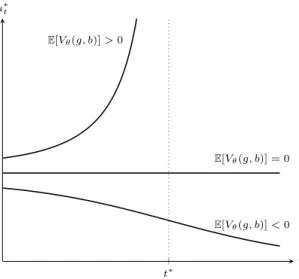
t∗ E[Vθ(g, b)] < 0 E[Vθ(g, b)] = 0 E[Vθ(g, b)] > 0 t µ∗t
Figure 1: Three branches of equilibrium investment rates.
Here, the mechanism is slightly different. Agents who hold private information have an incentive to experiment to conceal bad news from others to encourage them to experiment more. Accordingly, we label this effect as encouragement through signaling.
When the most optimistic belief p0(g, g) lies below the follower threshold, then agents invest
cautiously. Optimistic agents still invest, but with delay, because they benefit from the possibility, that the other invests first and then provides free information. Pessimistic agents strictly prefer to wait for the other agent to invest. Because different types invest with different probabilities, they separate gradually over time. While both agents wait for the first investment, they continuously update their beliefs about each other’s type. The longer an agent has waited, the more likely it is that she observed a bad signal.
The dynamics of investments are determined by the evolution of the agents’ belief about the state of the world θ. Each agent obtains information about the state from the investment behavior of the other. The longer the game proceeds without investment, the more pessemistic agents become both about type of the other agent and the state of the world. This change in beliefs in return affects their incentives to invest. The result of this mutual interaction is a learning feed-back loop. The effects of the feed-back loop can be seen in the dynamics of investment rates, illustrated in Figure ??. The upper branch represents the case in which the leader value is positive, even if the other agent’s signal was bad: E[Vθ(g, b)] > 0. If this is the case, then one agent’s inactivity has a motivating effect on the other. As agents become more convinced that the other agent’s type is bad, their value from waiting diminishes, and thus they are more willing to invest. This change in incentives is reflected by the increasing slope of investment rates. As investment rates increase, learning accelerates in a self-reinforcing manner and eventually explodes at a finite time t∗.
from immediate investment is negative. In this case, inactivity has a dampening effects on invest-ments. As agents become more convinced that the other’s signal is bad after a period of inactivity, it becomes more likely that their investment will result in losses. They are thus less willing to invest, and also reveal less information about their type. The investment rates eventually converge to zero, and type are never fully revealed in the long run.
That the investment rates are constant when E[Vθ(g, b)] appears natural in the diagram, but is not obvious a priori. Inactivity still makes agents more pessimistic about the state of the world. At the same time, the opportunity cost of waiting decreases. In equilibrium, these two effects balance each other out perfectly.
4 Welfare and transparency
The following theorem characterizes the cooperative benchmark, which corresponds to a setting in which agents pool their private information and commit to a strategy at the outset of the game, seeking to maximize the sum of their payoffs. We shall see that, when signals are publicly observable, all equilibria are ex-post efficient when the prior belief that the state is good is either very high or very low.
Theorem 3 (Cooperative benchmark). In the cooperative benchmark, both agents invest
immedi-ately if ˇp0 > p and never invest if ˇp0 < p. If ˇp0 = p, either solution is optimal.
Thus, as a comparison with the equilibrium in Theorem 2 shows, equilibrium under private information may be inefficient for intermediate prior beliefs. Inefficiencies arise because of leadership aversion: agents prefer being the follower and therefore wait if there is a sufficiently high probability that the other agent invests first. Free-riding aggravates its effect, because it lowers the value of being the leader, and thus reduces the rate at which the agents are willing to make the first investment.6 It is therefore natural to ask if there is a social gain from increasing transparency. Na¨ıve logic may suggest that more transparency should unambiguously lead to better outcomes, as it allows the agents to make better-informed decisions. This view, however, disregards the fact that agents wait inefficiently long for others to provide information for free when they are uncertain about the state, which negatively affects the efficiency of learning. Asymmetric information, as it turns out, can have positive side-effects. On the one hand, uncertainty introduces strategic risk about the other agent’s future investment decisions, which lowers the incentives to delay initial investments. On the other hand, when signals are private, an early investment can signal good news, giving rise to an encouragement-though-signalling effect, by which an agent invests in order to motivate her partner to invest as well. Thus, there is a tradeoff between the gains from information aggregation and limiting public access to information in order to reduce the agents’ incentives to free-ride.
6There is also a third type of inefficiency as agents may not invest in equilibrium although investment is optimal.
In the following, we state our main result, which formalizes this insight. It shows that private information is socially preferable if the prior belief that the state is good is high enough, and the signals are not too informative. To this end, denote by W0(s1, s2) the expected social surplus
generated in the unique symmetric equilibrium under public information, when p0(s1, s2) is the
common initial belief that the state is good. Let ˜W denote the ex-ante expected social surplus generated in a symmetric equilibrium in which each agent’s signal is private information. The following theorem shows that, for some parameters, ˜W ≥ E[W0(s1, s2)].
Theorem 4 (Welfare improvement through private information). Let p0 > p∗l. There exists a
ρ∗ > 1/2 such that, for all signal precisions ρ ∈ (1/2, ρ∗), we have ˜W ≥ E[W0(s1, s2)]. For
p∗l < p0 < p∗f, the inequality is strict.
The condition on the signal precision ensures that it is socially optimal for both agents to invest immediately. Thus uncertainty only affects strategic interaction. If p0 > p∗f, there always exists a range of signal precisions guaranteeing that both types invest immediately under private information, as in the efficient benchmark. If p0 < p∗f, then there signal precisions such that
the symmetric equilibrium has delayed entry. In this case, the welfare improvement results from strategic uncertainty and a spiraling effect, in which increasing pessimism about each other’s types and increasing eagerness to invest result in ex-ante earlier investment.
5 Conclusion
We have investigated how private information affects agents’ incentives to make irreversible in-vestments. Agents benefit from their partner’s experimentation because it provides them free information. However, delaying one’s investment can signal bad news, thus discouraging experi-mentation by one’s partner. We have shown that private information may increase social welfare in our setting by deterring delays in investments, as they may be interpreted as signaling bad news.
One might wonder about the impact of allowing communication between agents in our setting. We conjecture that allowing for cheap talk between agents would not change the outcome. Indeed, if it did, either agent would always send the most positive signal to induce the other one to invest early. We should furthermore anticipate communication with verifiable messages to lead to unraveling, as agents would prefer to communicate their signal only if it is good, so that each agent can infer the other agent’s signal perfectly. A deeper analysis of the role of communication in our setting would thus likely require that one abandon either our binary state space or the binary signal structure. We commend such an investigation to future research.
6 Proofs
Proof of Lemma 1. (i) That vl is linear in p is obvious from its definition inEquation (1) and vl is increasing in p because it follows from γc > y > 0 that the second term in Equation (1) is negative. To see that vl is decreasing in τ , note that λ2 < λ1, and hence
d
dτvl(p, τ ) =−(r + γ)(1 − p)(λ1− λ2)e
−(r+γ)τ(γc− y) < 0 for all p∈ (0, 1) and τ ≥ 0. That vl is convex in τ for all p∈ (0, 1) follows from
d2
d2τvl(p, τ ) = (r + γ)
2(1− p)(λ
1− λ2)e−(r+γ)τ(γc− y) > 0.
Finally, supermodularity holds because d2
dpdτvl(p, τ ) = (r + γ)(λ1− λ2)e
−(r+γ)τ(γc− y) > 0.
(ii) Linearity of vf in p is obvious from its definition in (2) and it is increasing in p because
γc > y > 0 implies that the first term in Equation (2)is positive and the second term is negative.
For fixed p∈ (0, 1), the derivative of vf with respect to τ is d dτvf(p, τ ) =−e −rτ[rpy− (r + γ)e−γτ(1− p)λ 2(cγ− y) ] .
Let ˆτ (p) be the (finite) solution to the first order condition dvf(p, τ )/dτ = 0. The second term in brackets is positive, so that dvf(p, τ )/dτ > 0 if τ < ˆτ (p) and dvf(p, τ )/dτ < 0 if τ > ˆτ (p). Hence, vf attains a global maximum at ˆτ (p). If ˆτ (p)≥ 0, then solving
rpy + (r + γ)e−γˆτ∗(p0)(1− p)(λ
2(y− cγ)) = 0
for ˆτ (p) shows that ˆτ (p) = τ∗(p). If ˆτ (p) < 0, then vf(p,·) is strictly decreasing on [0, ∞), and therefore assumes its maximum at 0.
(iii) If p < p∗f then τ∗(p) > 0. Since vl is strictly decreasing in τ and because τ∗(p) maximizes vf, we have vf(p, τ∗(p)) > vf(p, 0) = vl(p, 0) > vl(p, τ∗(p)). If p≥ p∗f, then τ∗(p) = 0, and therefore vf(p, τ∗(p)) = vf(p, 0) = vl(p, 0) = vl(p, τ∗(p)).
Proof of Lemma 2. From the definition of vf, it follows that vf(p, 0) > 0 if and only if p > p. Inspection reveals that p∗f > p which implies vf(p∗f, 0) > 0. Moreover, vl(p, 0) = vf(p, 0) for all p, and therefore v∗l(p∗f) = vl(p∗f, 0) > 0. Because vl is continuous and strictly increasing, it follows from v∗l(p∗l) = 0 that p∗l < p∗f. Moreover, we have 0 = vl∗(p∗l) < vl(p∗l, 0) = vf(p∗l, 0). By Lemma 1, vf is linearly increasing in its first argument. Since vf(p, 0) = 0, it follows from vf(p∗l, 0) > 0 that
p < p∗l.
Proof of Theorem 1. (i) Let ˇp0 ≥ p∗f. By definition of p∗f, the follower’s unique best response
is to invest as soon as the other player has invested. It remains to be shown that there exists no equilibrium in which both players either never invest or invest (simultaneously) at some time t > 0. If a player deviates to investing at time 0, she would get a payoff of w∗ = ˇp0y+(1− ˇp0)λ2(y−γc) > 0,
where the inequality holds because ˇp0 ≥ p∗f >
λ2(γc−y)
y+λ2(γc−y). In the conjectured equilibrium, by
contrast, she obtains e−rtw∗ < w∗ (t∈ (0, ∞) ∪ {∞}). Thus, she has an incentive to deviate and the only equilibrium is one in which both agents invest immediately.
(ii) Let p∗l < ˇp0< p∗f. By definition of p∗l, an agent would want to invest immediately if the other agent never invested. If the other agent invested, however, an agent would prefer not to invest, as this would give her vf∗(ˇp0) instead of vf(ˇp0, 0) < vf∗(ˇp0), where the inequality holds because of
ˇ
p0 < p∗f by definition of p∗f. As shown in the main text, there is a unique investment rate β∗(ˇp0)
that renders the other agent indifferent between investing and not investing, which establishes the claim.
(iii) For ˇp0≤ p∗l, the claim follows immediately from the definition of p∗l.
Lemma 3. v∗f(p)− v∗l(p) is a weakly decreasing function.
Proof. Define D(p, τ ) = vf(p, τ )− vl(p, τ ). If p≥ p∗f, then τ∗(p) = 0 and therefore D(p, τ∗(p)) = 0. Suppose p < p∗f. Taking the derivative gives
dD(p, τ∗(p)) dp = ∂D(p, τ∗(p)) ∂p + ∂D(p, τ∗(p)) ∂τ dτ∗(p) dp . (6)
Lemma 1implies that the leader value is decreasing in τ , i.e., dvl(p, τ∗(p))/dτ < 0, the optimal delay is decreasing, dτ∗(p)/dp < 0, and that τ∗(p) maximizes the follower value, i.e., dvf(p, τ∗(p))/dτ = 0. Therefore, D(p) is strictly decreasing on (0, p∗f) if ∂D(p, τ∗(p))/∂p < 0. Using the definition of vf inEquation (2), the derivative of the follower value is
∂vf(p, τ∗(p))
∂p = e
−rτ∗(p)
y + e−(r+γ)τ∗(p)λ2(γc− y).
FromEquation (1), the derivative of the leader’s value is ∂vl(p, τ∗(p))
∂p = y + (λ1+ (λ2− λ1)e
−(r+γ)τ∗(p)
)(γc− y).
The partial derivative of D with respect to p is ∂D(p, τ∗(p)) ∂p =−(1 − e −rτ∗(p) )y− λ1(1− e−(r+γ)τ ∗(p) )(γc− y) < 0.
Proof of Theorem 2.
Part (i). Suppose p0 > 0 and ρ > 1/2 such that p0(g, g) ≥ p∗f. We proceed to verify that the
following strategies and beliefs are part of an equilibrium. In the first phase, an agent with signal
g invests immediately. An agent with signal b invests immediately with probability η ∈ [0, 1].
With probability 1− η she invests at a random time drawn from an exponential distribution with parameter β∗(p0(b, b))∨0. In the second phase of the game, a follower with posterior belief p delays
investment by τ∗(p), and the beliefs at t are updated via Bayes’ rule whenever possible. A leader with signal g reverses her investment immediately at t = 0 if and only if her posterior belief about
θ is lower than p∗l. A leader with signal b reverses her investment immediately at t = 0 with some
probability ν ∈ [0, 1). Either agent exits in the second phase after the occurrence of a failure. In either phase, each agent i’s belief with signal s assigns probability p0(b, s) to state θ = H after an
off-equilibrium deviation of agent−i.
We show that there exist µ, ν such that above strategies and associated beliefs characterize a perfect Bayesian equilibrium. Consider first the second phase, taken as given that each type g invests at t = 0 with probability 1, and each type b invests at t = 0 with probability η and waits with probability 1−η. As shown in Lemma1, the function τ∗(p) is the optimal delay of the follower with posterior p, and thus given the leader stays in the game, a follower cannot gain from deviating in the second phase of the game. If the leader exits immediately in the second phase, the follower cannot influence that decision. In the second phase, suppose agent i with signal s invests at time
t = 0 in the first phase, and the other agent −i does not, so that at t = 0 in the second phase,
agent i is the leader and −i the follower. If both expect that the other agent follows the strategy described in the previous paragraph, then the posterior belief of agent i with signal s is p0(b, s),
and the posterior belief of type s of agent −i is, by Bayes’ rule, ˜
p(η, s) = p0(s)(ρ + η(1− ρ))
p0(s)(ρ + η(1− ρ)) + (1 − p0(s))(1− (1 − η)ρ)
. (7)
If vl(p0(b, b), τ∗(p(η, b))) > 0, then the continuation payoffs for either type of agent i is positive
(since vl(p0, τ∗(˜p(ην, b))) > vl(p0(b, b), τ∗(˜p(ην, b)))), and thus it is optimal for both types of agent i to stay in. If, on the other hand, vl(p0(b, b), τ∗(˜p(η, b))) < 0 < vl(p0(b, b), τ∗(p0)), then type b of
agent i remains in the game with probability ν∗ ∈ (0, 1) solving vl(p0(b, b), τ∗(˜p(ην∗, b))) = 0.7 If vl(p0(b, b), τ∗(p0)) < 0, then type b of agent i exits for sure, and type g remains if vl(p0, τ∗(p0)) = vl∗(p0)≥ 0. These actions are optimal for each agent by construction.
It remains to be shown that there exists a value for η such that neither agent can gain by deviating from the specified strategies in the first phase. Denote by Vθ(η) the value of investing
7
Note that ˜p(ην∗, b) is the posterior belief of type b of agent−i that the state is H, conditional on the joint event
that agent i invested in the first phase and remains in the second phase, where ην∗is the probability that type b of agent i does this.
at t = 0 for an agent in state θ, and let Wθ(η, τ ) be the value of waiting at t = 0 when the agent delays investment by τ as follower. Note here that τ refers to the delay of the investment, given that the other agent invests immediately at t = 0. When neither agent invests, then each agent is convinced that the other agents’ type is bad, and thus there is no longer any uncertainty about others’ private information. Note here that when the state and strategies are given, the payoff is independent of private signals. Note also that for a follower in the second phase, the optimal delay for each type b is τ∗(˜p(η, b)) when type b of the other agent invests with probability η. We write
Wθ∗(η) := max
τ Wθ(η, τ ) = Wθ(η, τ
∗(˜p(η, b)). for the payoff from waiting when using the optimal delay.
There is a pooling equilibrium if and only if p0(b)≥ p∗f, since in this case each type of each agent
is willing to invest immediately, if the other agent invests for sure, and thus reveals no information. Thus, consider the case p0(b) < p∗f. Note that in this case, we have E[Wθ∗(1)|b] ≥ E[Vθ(1)|b], since bad types always have weak incentives to wait when the other agent invests with probability one. There are two cases to consider, E[Wθ∗(0)|b] < E[Vθ(0)|b] and E[Wb∗(0)|b] ≥ E[Vθ(0)|b].
1.) SupposeE[Wθ∗(0)|b] < E[Vθ(0)|b], i.e., an agent with a bad signal prefers to invest immediately if the other agent invests with zero probability after a bad signal. gIn this case, there exists a partial (or full) pooling equilibrium in which type g always invests while type b invests with probability η∗ ∈ [0, 1]. Note that the functions E[Wθ∗(η)|b] and E[Vθ(η)|b] are convex combinations of continuous functions and hence continuous. Thus, there exists an η∗ ∈ (0, 1] such that E[Vθ(η∗)− Wθ∗(η∗)|b], so that an agent with type b is indifferent between investing and not investing, given the other agent invests with probability η∗ after observing signal b. We shall now verify an agent of type g’s incentives to invest. Note that we have the following inequality: 0 =E[Vθ(η∗)− Wθ∗(η∗)|b] ≤ E[Vθ(η∗)− Wθ(η∗, τ∗(˜p(η∗, g)))|b] = p0(b) ( VH(η∗)− WH(η∗, τ∗(˜p(η∗, g)) ) + (1− p0(b)) ( VL(η∗)− WL(η∗, τ∗(˜p(η∗, g))) ) ≤ p0(g) ( VH(η∗)− WH(η∗, τ∗(˜p(η∗, g)) ) + (1− p0(g)) ( VL(η∗)− WL(η∗, τ∗(˜p(η∗, g))) ) =E[Vθ(η∗)− Wθ∗(η∗)|g],
where the first inequality follows from the fact that E[Wθ∗(η∗)|b] ≥ E[Wθ(η∗, τ )|b] for all τ ≥ 0 by definition, and the second inequality from p0(g) > p0(b), and from the fact that investing
immediately is strictly better than waiting if and only if the state is H (since there is no gain from delay in state H, and no gain from investing in state L).
agent invests only if his signal is g. For agents with signal g in this case we have E[Vθ(0)− Wθ(0)|g] = q0(g) ( vl(p0(g, g), 0)− v∗f(p0(g, g)) ) + (1− q0(g)) ( 0∨ vl∗(p0)− 0 ∨ vl(p0, τ∗(p0(b, b)) ) . Since p0(g, g)≥ p∗f by assumption, we have vl(p0(g, g), 0)− vf∗(p0(g, g)) = 0, and thusE[Vθ(0)−
Wθ(0)|g] ≥ 0. Thus, in this case, we have a fully separating equilibrium in which g-types invest
at t = 0, whereas b-types do not.
Part (2.). Suppose p0> 0 and ρ∈ (1/2, 1) are such that p0(g, g) < p∗f. Consider again the second
phase first. The strategies outlines in the theorem constitute a separating equilibrium in the first phase, so that an agent who invests in the first phase and becomes the leader reveals to be of type g. Suppose that after type g of agent i invests at time t in the first phase, the agents use the following continuation strategy:
1. If vl∗(pt+∆)≥ 0, where ∆ = τ∗(p0(g, g)), and
pt+∆=
p0
p0+ (1− p0)e−γ∆ ,
then type g of agent i remains in the game indefinitely, and each type s of agent −i invests with delay τ∗(p0(s, g))
2. If v∗l(pt+∆) < 0 < vl(pt+∆, 0), then type g of agent i remains indefinitely if agent −i invests with delay τ∗(p0(g, g)) and exits otherwise. Each type of agent−i invests with delay ∆.8
3. If vl(pt+∆, 0) < 0, then type g of agent i remains in until t + ∆ if agent−i invests with delay ∆, and agent i exits otherwise. Type g of agent −i invests with delay ∆, and type b of agent −i invests with delay τ∗(p
0).
Henceforth, for each of the three cases above, denote by Vθ(si, s−i) the value of agent i con-ditional on (i) state θ, (ii) agent i following the strategy for agents with signal of becoming the leader conditional on the other agent being of type s−i, and let Wθ(si, s−i) be the value of be-coming the follower. Note that these payoffs are independent of time on the first phase, since the signal pair (si, s−i) encapsulates all information that is exchanged in the first phase, so that pt(si, s−i) = p0(si, s−i).
8
This case uses as threat that the leader cannot reinvest after dropping out. There also is a slightly more involved equilibrium that does not require this restriction. In this equilibrium, the agents enter another war of attrition, in which the follower delays investment in such a way that at each point in time, the leader is just willing to stay in, up until the optimal delay of the follower is reached. This would make the follower better off, and result in a welfare loss.
Thus, each agent’s expected value of becoming the leader is given by
U (qt(g)) = qt(g)E[Vθ(g, g)|si = g, s−i = g] + (1− qt(g))E[Vθ(g, b))|si= g, s−i = b].
Type g of each agent is willing to randomize if she is indifferent between investing immediately and waiting for another instant. Hence, the value function for type g of the agent must satisfy the indifference condition
U (qt(g)) = µtqt(g)E[Wθ(g, g)|si= g, s−i= g]dt + (1− rdt − µtqt(g)dt)U (qt+dt(g)). (8) By Ito’s Lemma, the indifference condition(8) can be written as
U (qt+dt(g)) = U (qt(g)) + dU (qt(g))dqt(g), (9) where by definition of U , we have dU (qt(g))/dqt(g) =E[Vθ(g, g)]− E[Vθ(g, b)]. Bayes’ rule implies that the posterior belief at t + dt is
qt+dt(g) = qt(g)(1− µtdt) 1− qt(g)µtdt . The differential change in belief is therefore
dqt(g)
dt ≡ limdt→0
qt+dt(g)− qt(g)
dt =−µtqt(g)(1− qt(g)). (10)
If we now substitute equations(9)and(10)in the indifference condition(8)and ignore higher order terms, we obtain the expression
rU (qt(g)) = µtqt(g)E[Wθ(g, g)− Vθ(g, g)|si = g, s−i = g]. (11)
Since p0(g, g) < p∗f, the right-hand side of this equation is strictly positive. Simplifying and solving
the equation for µt yields µt=
rU (qt(g))
qt(g)E[Wθ(g, g)− Vθ(g, g)|si = g, s−i= g]
. (12)
Here, µt is the rate of investment for type g of each agent in the symmetric equilibrium at a given belief qt(g). Substituting this last expression into Equation (10), we obtain the evolution of the posterior qt(g) in equilibrium:
dqt(g) =−(1 − qt(g)) rU (qt(g))
E[Wθ(g, g)− Vθ(g, g)|si = g, s−i= g]
We obtain the equilibrium belief and equilibrium investment rate at each time t by solving Equa-tion (13)with given initial belief q0.The initial value problem(13)has the unique solution
qt(g) = e −t ˆβU (q 0(g)) + (1− q0(g))E[Vθ(g, b) e−t ˆβU (q 0(g))− (1 − q0(g))E [Vθ(g, g)− Vθ(g, b)|si= g] . (14)
We now substitute qt(g)∗ intoEquation (12)and simplify to obtain the equilibrium rate of invest-ment µ∗t = e −t ˆβU (q 0(g)) e−t ˆβU (q 0(g)) + (1− q0)E[Vθ(g, b)|si= g] ˆ β. (15)
If rE[Vθ(g, b)] > 0 then the investment rate µ∗
t diverges to +∞ as t → t∗, where t∗= log ( 1 +p0(g, g) p0 E[Vθ(g, g)] E[Vθ(g, b)] )β∗(p0(g,g)) . (16)
If, on the other hand, E[Vθ(g, b)] < 0, thenEquation (15)converges to 0 as t→ ∞. Thus, t∗ =∞. It remains to be shown that it is optimal for type b of each agent to delay investment until t∗. For agents with signal b, the incremental opportunity cost from waiting isE[Vθ(b, s)|si = b]dt. The expected incremental gain from waiting for this type is µ∗tqt(b)E[Wθ(b, g)− Vθ(b, g)|si = b]dt. We show that when agents with signal g invest at rate µ∗t, then agents with signal b prefer to wait:
rE[Vθ(b, s)|si = b]≤ µ∗tqt(b)E[Wθ(b, g)− Vθ(b, g)|si = b, s−i = g]. (17) Because flow values are positive in state H and negative in state L, i.e., y ≥ 0 ≥ y − γc, we have VH(si, s−i)≥ 0 ≥ VL(si, s−i). Therefore:
Et[Vθ(si, s−i)|si = b] = pt(b)Et[VH(si, s−i)|si= b] + (1− pt(b))Et[VL(si, s−i)|si= b] ≤ pt(g)Et[VH(si, s−i)|si = b] + (1− pt(g))Et[VL(si, s−i)|si = b] ≤ pt(g)Et[VH(b, s−i)|si = g] + (1− pt(g))Et[VL(b, s−i)|si = g] ≤ pt(g)Et[VH(g, s−i)|si= g] + (1− pt(g))Et[VL(g, s−i)|si = g] =E[Vθ(si, s−i)|si = g].
The first inequality follows because pt(g) > pt(b). Note that according to our prescribed strategies, agents with signal g invest earlier than agents with signal b, and exit later. Therefore, we have Vθ(si, g)≥ Vθ(si, b). Since qt(g) > qt(b), we thus have E[Vθ(b, s−i)|si = g]≥ E[Vθ(b, s−i)|si = b] for each θ, which explains the second inequality. The last inequality follows because the strategy of
type g is constructed to maximize the continuation payoff after investing. Note that 1 qt(si)E[Vθ (si, s−i)|si] = pt(si) qt(si)E[VH (si, s−i)|si] + 1− pt(si) qt(si) E[VL (si, s−i)|si]
Because ρ > 1/2 and pt(g) > pt(b), it follows that pt(b) qt(b) = pt(b) ρpt(b) + (1− ρ)(1 − pt(b)) < pt(g) ρpt(g) + (1− ρ)(1 − pt(g)) = pt(g) qt(g) and similarly, 1− pt(b) qt(b) > 1− pt(g) qt(g) Combining the previous results, we find that
1 qt(b)E[Vθ (si, s−i)|si = b] = pt(b) qt(b)E[VH (si, s−i)|si = b] + 1− pt(b) qt(b) E[VL (si, s−i)|si= b] ≤ pt(g)
qt(g)E[VH(si, s−i)|si = b] +
1− pt(g) qt(g) E[VL(si, s−i)|si = b] ≤ pt(g) qt(g)E[VH (si, s−i)|si = g] + 1− pt(g) qt(g) E[VL (si, s−i)|si= g] = 1 qt(g)E[Vθ (si, s−i)|si = g]
The previous inequalities, together with(11), imply 1
qt(b)rE[Vθ(si, s−i)|si= b]≤ 1
qt(g)rE[Vθ(si, s−i)|si= g] (18)
= µ∗tE[Wθ(g, g)− Vθ(g, g)|si = g, s−i = g]. (19) On the other hand, again by y > 0 > y− γc, waiting has negative value in state H, and positive value in state L, so that
WH(si, g)− VH(si, g)≤ 0 ≤ WL(si, g)− VL(si, g). (20)
The continuation payoff E[Wθ(b, g)|si = b] for agent i with signal b in the event that agent −i invests must maximize i’s payoff, and therefore,
E[Wθ(g, g)|si = b]≤ E[Wθ(b, g)|si = b]. (21)
we have
E[Vθ(si, s−i)|si = b, s−i = g]≥ E[Vθ(g, s−i)|si = b, s−i= g]. (22) It then follows that
1 qt(b)
rE[Vθ(si, s−i)|si = b] < µ∗tE[Wθ(si, s−i)− Vθ(si, s−i)|si = g, s−i = g] ≤ µ∗
tE[Wθ(g, s−i)− Vθ(g, s−i)|si = b, s−i = g] ≤ µ∗
tE[Wθ(si, s−i)− Vθ(si, s−i)|si = b, s−i= g]
The first inequality follows from(18). The second inequality follows from(20). The last inequality follows from(21) and (22). The chain of inequalities implies (17)shich was to be shown.
Part (3.). As before, the function τ∗(p) is the optimal delay of the follower with posterior p, and
thus given the leader stays in the game, a follower cannot gain from deviating in the second phase of the game. Assuming that the follower always uses delay τ∗(p) at posterior p, the value of becoming the leader for an agent with signal g is E[vl∗(p0(b, s))|g]. If this value is negative, then no agent is
willing to become a leader, so no investment takes places at any t≥ 0.
Proof of Theorem 3. The team’s objective is to maximize w(p, τ ) = max{0, vl(p, τ ) + vf(p, τ )} ,
where τ denotes the delay with which the follower invests. Vsing Equations (1) and (2), we can write explicitly: w(p, τ ) = (1 + e−rτ)py + (1− p) [ λ1+ (2λ2− λ1)e−(r+γ)τ ] (y− γc).
It follows from the definitions of λ1 and λ2 that 2λ2− λ1 = λ1λ2. Therefore, the marginal value of
delaying the second investment is ∂w(p, τ )
∂τ =−re
−rτ[py + (1− p)λ
2(y− γc)e−γτ]. (23)
The expression in brackets is strictly increasing in τ . This implies that ∂w(p, τ )/∂τ < 0 for all
τ ≥ 0 whenever p > p, where
p := λ2(γc− y)
y + λ2(γc− y)
, (24)
in which case it is socially optimal to make the second investment immediately. If p≤ p, then the socially optimal delay solves the first-order condition dw(p, τ )/dτ = 0. Thus, the optimal delay is
given by τs(p) = [ϕ(p)− ϕ(p)]/γ if p < p, 0 if p≥ p.
It remains to be shown that, if p≤ p, w(p, τs(p)) = 0. Indeed,
w(p, τs(p)) = max { py + (1− p)λ1(y− γc) + py ( 1− λ1 1− p ) ( p(1− p) p(1− p) )r γ , 0 } .
Since p ≤ p, it is sufficient to show that py + (1 − p)λ1(y − γc) + py (1 − λ1/(1− p)) ≤ 0 and
py + (1−p)λ1(y−γc) ≤ 0. As both inequalities are satisfied for p ≤ p, this concludes the proof.
Proof of Theorem 4. Let P be the distribution over signals for given parameters p0 and ρ. We
write P (s) for the probability that a given agent’s signal is s and P (s1, s2) for the probability that
the pair of signals is (s1, s2).
(1.) Suppose p0 > p∗f. Then, choose ρ∗ > 1/2 such that p0(b) > p∗f and p0(b, b) > p. ByTheorem 2,
it follows that for all ρ < ρ∗, there exists a pooling equilibrium in which each type of each agent invests immediately. ByTheorem 3, this equilibrium is efficient. Hence ˜W ≥ E[Wθ(s1, s2)].
(2.) Let p∗f > p0 > p∗l. Choose ρ∗ > 1/2 such that p∗f > p0(g, g) and p0(b, b) ≥ p. By
The-orem 2, there exists an equilibrium with delayed entry. It follows from arguments in the proof of Theorem 2 that the expected equilibrium value of the good type of each agent is E[Vθ(g, s−i)] ≥ E[vl∗|g]. The inequality follows from the fact that leaders have the option to exit. By Equation (17), bad types strictly prefer to delay investment at each t < t∗. The expected payoff for an agent of type b who deviates by investing before time t∗ is given by
qt(b)vl(p0, τ∗(p0(g, g))) + (1− qt(b))v∗l(p0(b, b), τ∗(p0)) >E[vl∗|b]. Therefore, the expected social surplus for each agent is
˜
W > P (g)E[v∗l|g] + P (b)E[v∗l|b] = E[Wθ(s1, s2)].
(3.) Let p0 = p∗f. Since p0(g, g) > p∗f, each agent with signal g invests immediately. For ρ close to
1/2, agents with type g never exit in equilibrium. We show that there exists ρ∗ > 1/2 such that ˜W > E[Wθ(s1, s2)] for all ρ ∈ (1/2, ρ∗). The equilibrium is with immediate investment,
since p0(g) > p∗f. There cannot be a pooling eqilibrium, since p0(b) < p0 = p∗f. If it was fully
separating, then an agent with signal b would strictly prefer to invest immediately to induce the other agent to invest. Hence it must be partially separating. By indifference for type b,
we can write the social welfare per agent as ˜ W = P (g) [ q0(g)vl(p0(g, g), 0) + (1− q0(b))(ηvl(p0, 0) + (1− q0(g))(1− η)vl(p0, τ∗(˜pη(b)) ] + P (b) [ q0(b)vl(p0, 0) + (1− q0(b))(ηvl(p0(b, b), 0) + (1− η)(vl(p0(b, b), τ∗(pη(b))) ] . Note that P (g)q0(g) = P (g, g), P (g)(1− q0(g)) = P (b)q0(b) = P (b, g) and P (b)(1− q0(b)) = P (b, b). Using q0(b)p0 + (1− q0(b))p0(b, b) = p0(b) together with the linearity of vl(p, 0), we can write ˜ W = P (g, g)vl(p0(g, g), 0) + P (b, g)vl(p0, 0) + (P (g, b) + P (b, b)) [ ηvl(p0(b), 0) + (1− η)vl(p0(b), τ∗(˜p(η, b)) ] . When signals are public, then, after each realized pair of signals resulting in the posterior belief ˇp0, each agent’s equilibrium payoff is v∗l(ˇp0). Thus, the expected welfare under public
information can be written as
E[Wθ(s1, s2)] = P (g, g)vl∗(p0(g, g)) + P (b, g)v∗l(p0) + (P (g, b) + P (b, b)) [ q0(b)vl∗(p0) + (1− q0(b))v∗l(p0(b, b)) ] . (25)
Using the definition of τ∗ inLemma 1, we have
vl∗(p) = vl(p, τ∗(p)) = py + (1− p)λ1(y− γc) + (1 − p)e−(r+γ)τ
∗(p)
(λ2− λ1)(y− γc).
Since p0= p∗f, we have τ∗(p0) = τ∗(p0(g, g)) = 0. We have that ˜W > E[Wθ(s1, s2)] iff
ηvl(p0(b), 0)+(1−η)vl(p0(b), τ∗(˜p(η, b)) > q0(b)vl(p0, 0)+(1−q0(b))vl∗(p0(b, b))). (26)
We define ψ(p) := 1−pp = eϕ(p) and α := r+γγ > 1. Then, the left-hand side of Inequality (26)
can be written as ηvl(p0(b), 0) + (1− η)vl(p0(b), τ∗(˜p(η, b)) = p0(b)y + (1− p0(b))λ1(y− γc) + (1− p0(b)) [ η + (1− η)ψ(˜p(η, b))αψ(p∗f)−α ] (λ2− λ1)(y− γc) (27)
From Bayes’ rule and the definition of ψ, we have ψ(p0(b)) = p0 1− p0 1− ρ ρ = ψ(p0)/ψ(ρ), ψ(˜p(η, b)) = ψ(p0(b)) ( ρ + (1− ρ)η 1− ρ + ρη ) .
If we now use the previous equalities to factor out ψ(p0(b))αψ(p∗f)−α from the square brackets in(27), we obtain ηvl(p0(b), 0) + (1− η)vl(p0(b), τ∗(˜p(η, b)) = p0(b)y + (1− p0(b))λ1(y− γc) + (1− p0(b))ψ(p0(b))αψ(p∗f)−α [ ηψ(ρ)α+ (1− η) ( ρ + (1− ρ)η 1− ρ + ρη )α] (λ2− λ1)(y− γc). (28)
The right-hand side of Inequality(26) is given by
q0(b)vl(p0, 0)+(1− q0(b))vl∗(p0(b, b)) = p0(b)y + (1− p0(b))λ1(y− γc) + [ q0(b)(1− p0) + (1− q0(b))(1− p0(b, b))ψ(p0(b, b))αψ(p∗f)−α ] (λ2− λ1)(y− γc). (29)
From Bayes’ rule it follows that q0(b) 1− p0(b) = p0(b)ρ + (1− p0(b))(1− ρ) 1− p0(b) = ( p0 1− p0 1− ρ ρ ) ρ + (1− ρ) = 1− ρ 1− p0 , 1− q0(b) 1− p0(b) = p0(b)(1− ρ) + (1 − p0(b))ρ 1− p0(b) = ( p0 1− p0 1− ρ ρ ) (1− ρ) + ρ = ρ 1− p0(b, b) . Using these equalities together with the identity
ψ(p0(b, b)) =
p0(b)
1− p0(b)
1− ρ
ρ = ψ(p0(b)ψ(1− ρ)
to factor out (1− p0(b))ψ(p0(b))αψ(p∗f)−α from the square brackets in (29), we obtain
q0(b)vl(p0, 0) + (1− q0(b))vl∗(p0(b, b)) = p0(b)y + (1− p0(b))λ1(y− γc) + (1− p0(b))ψ(p0(b))αψ(p∗f)−α [ (1− ρ)ψ(ρ)α+ ρψ(ρ)−α ] (λ2− λ1)(y− γc).
Define the functions,
h(η, ρ) := ηψ(ρ)α+ (1− η) ( ρ + (1− ρ)η 1− ρ + ρη )α , g(ρ) := (1− ρ)ψ(ρ)α+ ρψ(ρ)−α.
Condition (26) is thus equivalent to infηh(η, ρ) > g(ρ). One calculates that the partial derivative of h at ρ = 1/2 is limρ→1/2∂ρh(η, ρ) = 4α
(
2η2− η + 1)/(η + 1). The function
limρ→1/2∂ρh(η, ρ) has its minimum in η at
√
2− 1 and is thus larger than 4(4√2− 5) > 0. On the other hand g′(1/2) = 0. Thus, there exists a ρ∗ > 1/2 such that for all ρ∈ (1/2, ρ∗), we have ˜W > E[Wθ(s1, s2)].
References
Bolton, P. and Harris, C. (1999). Strategic experimentation. Econometrica, 67(2):349–374. Bonatti, A. and H¨orner, J. (2011). Collaborating. American Economic Review, 101(2):632–63. Chamley, C. and Gale, D. (1994). Information Revelation and Strategic Delay in a Model of
Investment. Econometrica, 62(5):1065–85.
D´ecamps, J.-P. and Mariotti, T. (2004). Investment timing and learning externalities. Journal of Economic Theory, 118(1):80–102.
Heidhues, P., Rady, S., and Strack, P. (2015). Strategic experimentation with private payoffs. Journal of Economic Theory, 159:531–551.
Keller, G. and Rady, S. (2010). Strategic experimentation with Poisson bandits. Theoretical Economics, 5(2):275–311.
Keller, G. and Rady, S. (2015). Breakdowns. Theoretical Economics, 10(1):175–202.
Keller, G., Rady, S., and Cripps, M. (2005). Strategic Experimentation with Exponential Bandits. Econometrica, 73(1):39–68.
Morris, S. and Shin, H. H. S. (2002). Social Value of Public Information. The American Economic Review, 92(5):1521–1534.
Moscarini, G. and Squintani, F. (2010). Competitive experimentation with private information: The survivor’s curse. Journal of Economic Theory, 145(2):639–660.
Murto, P. and V¨alim¨aki, J. (2011). Learning and Information Aggregation in an Exit Game. The Review of Economic Studies, 78(4):1426–1461.
Murto, P. and V¨alim¨aki, J. (2013). Delay and information aggregation in stopping games with private information. Journal of Economic Theory, 148(6):2404–2435.
Rosenberg, D., Salomon, A., and Vieille, N. (2013). On games of strategic experimentation. Games and Economic Behavior, 82:31–51.
Rosenberg, D., Solan, E., and Vieille, N. (2007). Social Learning in One-Arm Bandit Problems. Econometrica, 75(6):1591–1611.
Teoh, S. (1997). Information disclosure and voluntary contributions to public goods. RAND Journal of Economics, 28(3):385–406.