THÈSE
En vue de l’obtention du
DOCTORAT DE L’UNIVERSITÉ DE
TOULOUSE
Délivré par :
Université Toulouse - Jean Jaurès
Présentée et soutenue par :
Sami MNASRI
le
mercredi 27 Juin 2018
Titre :
Contributions to the optimized deployment of connected sensors
on the Internet of Things collection networks
École doctorale et discipline ou spécialité :
ED MITT : Domaine STIC : Réseaux, Télécoms, Systèmes et Architecture
Unité de recherche :
Institut de Recherche en Informatique de Toulouse (IRIT), équipe RMESS
Directeur de Thèse :
Thierry VAL, Professeur à l'Université de Toulouse
Jury :
Pr. Belhassen ZOUARI, Université de Carthage, Rapporteur
HDR Dr. Hanen IDOUDI, Ecole Nationale des Sciences de I'nformatique de Tunis, Rapporteur Dr. Najeh NASRI, Ecole Nationale d'Ingénieur de Sfax, Co-Directeur de thèse
Nothing is stronger than a high-quality education system that can be the basis of building
human being in order to reform morals towards modern civilizations and nations
Sami Mnasri
To my mother and my father, To my sisters and my brother, To Ameni,
To my friends,
In testimony of my great love
and my strong gratitude
Sami
Acknowledgements
I would first like to thank Pr. Thierry VAL, my thesis director for his support
and contribution in this research as well as for his availability. In particular, I
thank him for giving me a great freedom in my research, for being attentive to
all my comments or ideas and for answering my many questions. His
encouragement and advices were invaluable, without which this work would
probably not have been possible.
I thank Dr Nejah NASRI for his interest in my work as well as for his comments
and advices which allowed me to improve the substance and form. I would like
to thank Dr. Adrien VAN DEN BOSSCHE for his advice and guidelines,
especially at the level of experiments and prototyping that have enhanced my
work.
I also thank Pr. Belhassen ZOUARI and Dr. Hanen IDOUDI for agreeing to be
part of my evaluation committee.
My thanks also go to all the teachers, staff and my students on the IUT of
Blagnac for the good atmosphere they created in the premises of the IUT.
Finally, I thank all the teachers who contributed to my training and to all those
who helped me during this work.
IoT collection networks raise many optimization problems, in particular because the sensors have limited capacity in energy, processing and memory. We are interested in a global contribution related to the optimization on wireless sensor networks using heuristics, meta-heuristics, hybrid methods, mathematical models, assessments of new optimization approaches on wireless sensor networks, multi-objective models, etc.
The continuous evolution of the IoT collection network research domain and technology allows optimizing the use of these networks in different number of contexts. The general problem of deployment of nodes can be described as follows: often, the sensors constituting the network cannot be precisely positioned and are scattered erratically. In order to compensate the randomness of sensor placement and increase the fault tolerance of the network, these sensors can be deployed intelligently. Unlike 3D deployment, there is a very abundant literature on this problem for 2D deployment ranging from the technical specificities of the sensors and their way of communicating, to the topological organization of the network itself. The 3D deployment of wireless sensors poses many optimization problems. Therefore, the goal is to provide 3D sensor organization solutions and find the most optimized architecture in order to improve the network performance.
In this context, heuristic approaches for optimization in wireless sensor networks can be envisaged. In addition, optimization problems are generally derived from real problems that are often antagonistic, unmeasurable and include several criteria. The dynamic, distributed and open aspect of the deployment problem led us to adopt advanced modeling and optimization technologies: hybridizing recent meta-heuristics. Indeed, in order to ensure a continuous evolution, a pragmatic flexibility and an infallible robustness against possible disturbances that could affect all or part of the network, the main goal was to propose hybridizations and modifications of the evolutionary optimization algorithms in order to achieve the positioning of nodes in wireless sensor networks with satisfaction of a set of constraints and objectives. In fact, hybrid meta-heuristics exploit the complementarity of these methods with each other, as well as with other "classical" approaches. This new class of hybrid algorithms has proven its robustness and efficiency in solving difficult optimization problems. We propose to focus our contribution composed of several complementary and progressive approaches, on the hybrid meta-heuristics. Especially on the evaluation of their performances and their applications on our real-world problem. These hybridization schemes are all validated by numerical results by the evaluation of algorithms with metrics such as the Hypervolume. Then, simulations supplemented by real experiments on testbeds were proposed. Finally, simulations are confronted with experiments to evaluate the behavior of algorithms and prove their stability and efficiency.
Keywords: 3D indoor deployment, ant colony algorithm, dimensionality reduction, experimental validation, genetic algorithms, hybridization, IoT collection networks, meta-heuristics, optimization, particle swarm optimization, user preferences.
Acknowledgements
About this dissertation ... i
Contents ... ii
List of figures ... v
List of algorithms ... vii
List of tables ... viii
List of acronyms ... ix
Introduction and Overview 1
Motivations and problematic ... 1
Research aims and principal contributions ... 2
Structuring of the document ... 4
I State of the Art 5
1 The 3D indoor deployment problem in WSN and DL-IoT collection networks 6
1.1 Introduction ... 7
1.2 Presentation, migration from WSN to DL-IoT and complexity of the deployment problem ...7
1.3 The 3D deployment strategies in WSN ...10
1.3.1 Full coverage ... 10
1.3.2 K-coverage ... 11
1.3.3 Surface coverage ... 11
1.4 Conflicting types of deployments ...11
1.4.1 Single Objective deployment vs. multi-objective deployment ... 11
1.4.2 Deterministic deployment vs. stochastic deployment ... 12
1.4.3 Stationnary deployment vs. mobile deployment ... 12
1.4.4 Homogenous deployment vs. heterogeneous deployment ... 12
1.4.5 Static deployment vs. dynamic deployment ... 13
1.5 Initial objectives to be satisfied during deployment ...13
1.5.1 The number of deployed nodes, cost and scalability ... 13
1.5.2 Coverage problem ... 14
1.5.3 Connectivity problem ... 15
1.5.4 Coverage with Connectivity ... 16
1.5.5 Energy efficiency ... 16
1.5.6 Network lifetime ... 17
1.5.7 Network traffic... 17
1.5.8 Data fidelity ... 17
1.5.9 Fault tolerance and load balancing ... 18
1.5.10 Latency ... 18
1.6 Sensing models ...18
1.6.1 Binary model ... 18
1.6.2 Probability model ... 19
1.6.3 Tracking detection model ... 19
1.6.4 Coverage and connectivity model ... 20
1.7 Open deployment issues ...20
1.8 Applications of the deployment ...23
1.9 Methodologies for solving the problem of deployment ...25
1.9.1 Virtual Force algorithms ... 25
1.9.2 BDA, PFDA and DDA Algorithms ... 26
1.9.3 Heuristic optimization ... 26
1.10 Other problems similar to the node positioning problem ...26
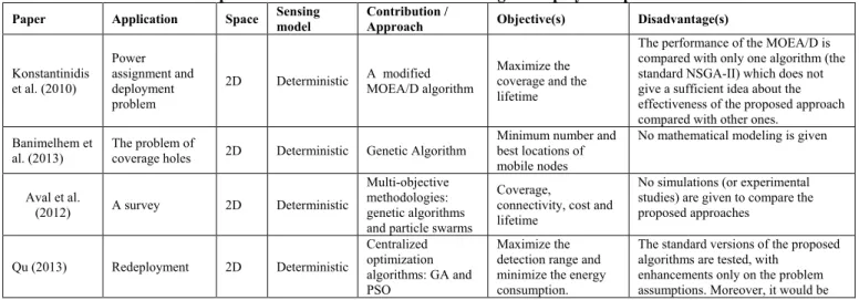
1.11 Comparaison and review of recent studies on WSN deployment ...27
2.2 Combinatorial optimization ...31
2.2.1 Complexity of a problem ... 31
2.2.2 Classification of optimization problems ... 31
2.3 Multi-objective optimization ...32
2.3.1 Pareto Optimality Concepts ... 33
2.3.2 Approaches to solve multi-objective optimization problems ... 34
2.3.2.1 Transformation of a multi-objective problem into a single objective problem ...34
2.3.2.2 Non-Pareto approaches (non-aggregated) ...36
2.3.2.3 Pareto approach ...37
2.4 Methods for solving multi-objective optimization problems ...37
2.4.1 Exact methods ... 37
2.4.2 Meta-heuristics ... 38
2.4.2.1 Taboo Search (TS) / Simulated Annealing (SA) ...38
2.4.2.2 Swarm Intelligence (ACO, PSO, BSO) ...39
2.4.2.3 Genetic algorithms (NSGA-II as an exemple) ...43
2.4.3 Many-objective optimization ... 46
2.4.3.1 Many-objective PSO algorithm ...47
2.4.3.2 NSGA-III algorithm ...47
2.4.3.3 MOEA/DD ...48
2.4.3.4 Two_Arch2 algorithm ...48
2.4.3.5 Similitudes and differences between many-objective algorithms ...49
2.4.3.6 Difficulties in MaOAs ...50
2.4.4 Hybridization of Meta-heuristics ... 51
2.4.4.1 Hybridization between metaheuristics ...51
2.4.4.2 Hybridization of Meta-heuristics and Exact Methods ...52
2.4.5 Relationship between the deployment problem and the multi-objective optimization………..52
2.5 Multi-agent Systems ...53
2.6 Preferences incorporation ...56
2.6.1 Generalities ... 56
2.6.2 Interactive preferences (PI-EMO-PC) ... 57
2.7 Dimensionality reduction ...58
2.7.1 Generalities ... 58
2.7.2 Offline correlation reduction methods based on machine learning for the 3D deployment problem ... 59
2.8 Conclusion ...59
II Contributions 60
3 Theoretical contributions 61
3.1 Introduction ...62
3.2 Mathematical model of the 3D indoor deployment in DL-IoT collection networks ...62
3.2.1 Architecture of nodes, assumptions, notation and objective function ... 62
3.2.1.1 Architecture of nodes ...62
3.2.1.2 Assumptions ...62
3.2.1.3 Notation ...63
3.2.1.4 The objective function ...65
3.2.2 The details of the objectives ... 65
3.3 Hybridizations and modifications on the optimization approaches for the 3D deployment ...71
3.3.1 Chromosome coding for the proposed MaOEAs ... 71
3.3.2 Inclusion of diversity ... 72
3.3.2.1 Neighbourhood restriction and adaptive multi-operators ...72
* Principles of the mutation and recombination with the neighbourhood (AxN and AmN) ...72
* Implementation of the AxN and AmN strategies on the proposed algorithms ...74
3.3.2.2 Including single-grid and mutiple scalarizing functions in the aggregation based approach ...76
3.3.3 Incorporation of Dimensionality Reduction (the NL-MVU-PCA algorithm) ... 77
3.3.3.1 Incorporating L-PCA and NL-MVU-PCA on the tested EMOs ...77
3.3.3.2 Integrating PI-EMO-PC, Knee points and NL-MVU-PCA on the proposed EMOs ...77
3.3.4 Incorporation of preferences ... 78
3.3.4.1 PI-NSGA-III-VF (NSGA-III with interactive preferences) ...79
3.3.6.1 The bird accent concept ...84
3.3.6.2 The accent measure ...85
3.3.6.3 The clustering in multiple Swarms ...85
3.3.7 Hybridizing Particle Swarm Optimization and Multi-Agent Systems ... 86
3.3.7.1 Multi-agent Systems ...86
3.3.7.2 The advantage of using the multi-agent approach in our context ...86
3.3.7.3 The acMaMaPSO: A hybrid algorithm based-on accent multi-agent many-objective PSO ...87
3.4 Conclusion ...90
4 Numerical results, simulations and experimentations on testbeds 91
4.1 Introduction ...92
4.2 Numerical results of incorporating dimensionality reduction and preferences on the deployment problem ...92
4.2.1 Results on a constrained real world problem: the 3D Deployment in indoor WSNs ... 94
4.2.1.1 Testing the effect of interdependence between objectives ...94
4.2.1.2 Testing the effect of the population size ...95
4.2.1.3 Testing the effect of the choice of the scalarizing functions in MOEA/D ...96
4.2.1.4 Testing the effect of using neighborhood mating and adaptive recombination operators ...97
4.2.1.5 Testing the effect of hybridizing the 5EMOs with a dimensionality reduction approach ...97
4.2.1.6 Testing the effect of hybridizing the EMOs with dimensionality reduction and user preferences .. 100
4.2.1.7 Results on PI-NSGA-III-VF ... 101
4.3 Numerical results on unconstrained DTLZ test functions ... 102
4.4 Simulations: Modeling the used protocols, simulation with small and large instances ... 109
4.4.1 Network protocol modeling ... 109
4.4.2 Small-scale simulations of the network with OMNet ++ ... 111
4.4.3 Large scale network simulations with OMNet++ ... 114
4.4.3.1 Variations in the number of nomad nodes added in large-scale simulations ... 115
4.4.3.2 Changes in RSSI rates in large-scale simulations ... 116
4.4.3.3 Variations in FER rates in large-scale simulations ... 116
4.4.3.4 Variations in the number of neighbors in large-scale simulations ... 117
4.4.3.5 Variations in energy consumption and network lifetime in large-scale simulations ... 117
4.4.4 Discussion and interpretations ... 118
4.5 Experimentations on real testbeds ... 119
4.5.1 Experimental parameters and used tools ... 119
4.5.2 Scenario 1: Testing with 11 nodes ... 121
4.5.2.1 Network architecture ... 121
4.5.2.2 Objectives ... 123
4.5.2.3 Variation of the localization ... 123
4.5.2.4 Variation of the coverage ... 124
4.5.2.5 Variation of the number of neighbors ... 125
4.5.2.6 Discussion ... 126
4.5.3 Scenario 2: Ophelia testbed (Testing with 36 nodes) ... 127
4.5.3.1 Experimental scenario and results ... 127
4.5.3.2 Interpretations and discussion ... 129
4.5.4 Results of experimentations on PI-NSGA-III ... 129
4.6 Results on hybridizing ACO and NSGA-III (AcNSGA-III) ... 130
4.6.1 Numerical results of the algorithms ... 130
4.6.2 Comparing simulations and experimentations ... 131
4.7 Results on accentBirdsPSO and on hybridizing PSO and MAS ... 134
4.7.1 Numerical results ... 134
4.7.2 Experimental and simulation results ... 136
4.8 Conclusion ... 138
Conclusions and future research directions ... 139
Publications ………...142
Bibliography ...………...…..144
Appendix 1 RSSI and FER measures of the experimental tests (Scenario 1) ….……….. 154
Figure 1.1 An example of area coverage using randomly deployed sensors ………...………8
Figure 1.2 2D deployment vs. 3D deployment ………...8
Figure 1.3 Phases of deployment………10
Figure 1.4 Different geometric 3D coverage layouts………..11
Figure 1.5 3D surface coverage………...11
Figure 1.6 Mobility taxonomy………...……….12
Figure 1.7 Coverage types………...15
Figure 1.8 Binary sensing model……….18
Figure 1.9 Probability sensing model………..19
Figure 1.10 Guaranteed-connectivity scheme (a) and guaranteed-coverage scheme (b)………20
Figure 1.11 Deployment of an underwater WSN………21
Figure 1.12 Smart homes ..………..25
Figure 2.1 Example of dominance………..33
Figure 2.2 Pareto front for a bi-objective problem………..33
Figure 2.3 Pareto Solutions……….…34
Figure 2.4 ε-contsraint method………35
Figure 2.5 Classification of multi-objective optimization methods ………...36
Figure 2.6 Displacement of a particle ………40
Figure 2.7 General architecture of a genetic algorithm………...44
Figure 2.8 NSGA-II Steps………...46
Figure 2.9 Flow-chart of the Two_Arch2 Algorithm………..49
Figure 2.10 Classes of Hybridization………..51
Figure 2.11 Schematization of an agent………..54
Figure 2.12 Multi-agent System………..…54
Figure 3.1 The 3D DV-HOP and RSSI protocol……….63
Figure 3.2 Different orientation positions of antennas………70
Figure 3.3The chromosome representing the sensor in the 3D position (46, 53, 34)……….………72
Figure 3.4 The four steps of the proposed hybridization scheme………...…78
Figure 3.5 Flowchart of the PI-NSGA-III-VF………...80
Figure 3.6 The proposed hybrid preference algorithm (PI-EMO-PC-INK)………....81
Figure 3.7 Nadir and ideal objective points………..…..…82
Figure 3.8 The choice of the neighborhood of a particle Pa………..….…85
Figure 3.9 The proposed MAS architecture………... 88
Figure 4.1: Localization algorithm with 3D DV-HOP + RSSI……….109
Figure 4.2 Small-scale simulation scenario………...112
Figure 4.3 Average RSSI rates during small-scale simulations………112
Figure 4.4 Average FER rates in small-scale simulations……….…113
Figure 4.5 Average number of neighbors in small-scale simulations………...113
Figure 4.6 Variation of energy in relation to the number of fixed nodes, for 2 objectives………...113
Figure 4.7 Variation of energy in relation to the number of fixed nodes, for 4 objectives………...114
Figure 4.8 Change in lifetime in relation to the time………114
Figure 4.9 Experiments vs. simulations for small scale instances………...…….114
Figure 4.10 Large-scale simulation scenario (85 fixed nodes and 36 nomad nodes) ………..115
Figure 4.11 Variations in the number of nomad nodes added for two objectives……….115
Figure 4.12 Variations in the number of nomad nodes added for four objectives………115
Figure 4.13 Average RSSI rates for different number of objectives……….116
Figure 4.14 Average RSSI rates according to the number of initial nodes………...116
Figure 4.15 Average FER rates for different number of objectives………..116
Figure 4.16 Average FER rates according to the number of initial node…………..………116
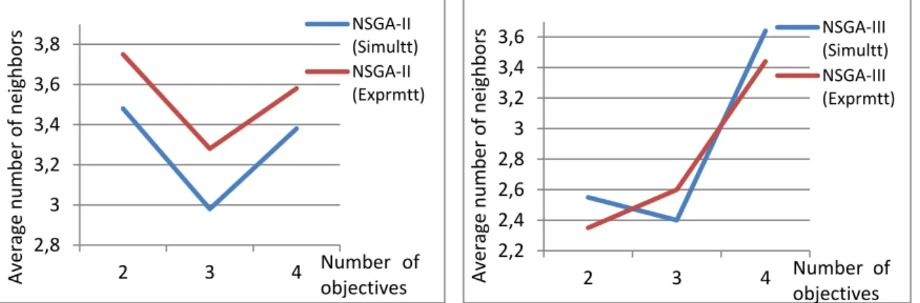
Figure 4.17 Average numbers of neighbors for three objectives………..117
Figure 4.18 Average numbers of neighbors for nine objectives………...117
Figure 4.19 Variation of energy in relation to the number of fixed nodes, for two objectives……….117
Figure 4.23 The logical network architecture………...121
Figure 4.24 The 2D and 3D architecture of the real deployed indoor network………122
Figure 4.25 Variations on the localization (RSSI), by day, for different positions………..124
Figure 4.26 Variations on the localization (RSSI), by night, for different positions………....124
Figure 4.27 Variations of the coverage (FER), by day, in different positions………..125
Figure 4.28 Variations of the coverage (FER), overnight, in different positions……….125
Figure 4.29 Variation of the number of neighbors, by day………..….125
Figure 4.30 Variation of the number of neighbors, by night……….125
Figure 4.31 The average RSSI values, for different number of objectives………...127
Figure 4.32 The average FER values, for different number of objectives………128
Figure 4.33 Average number of neighbors, for different number of objectives………...128
Figure 4.34 Average lifetime of the network, for different number of objectives………128
Figure 4.35 Average energy consumption levels, as a function of time………...128
Figure 4.36 Average rates of RSSI………...129
Figure 4.37 Average rates of FER……….130
Figure 4.38 Average number of neighbors………130
Figure 4.39 Comparing the average RSSI rates………132
Figure 4.40 Comparing the average FER rates……….133
Figure 4.41 Comparing the average number of neighbors………133
Figure 4.42 Comparing the average energy consumption levels………..133
Figure 4.43 Comparing the average lifetime……….133
Figure 4.44 RSSI average rates of nodes in connection with the mobile node……….137
Figure 4.45 FER average rates of nodes in connection with the mobile node………..137
Figure 4.46 Average number of neighbors of nodes in connection with the mobile node………...137
Algorithm 2.1 Simulated Annealing algorithm ………..38
Algorithm 2.2 Tabu Search algorithm……….39
Algorithm 2.3 Ant Colony Optimization algorithm………40
Algorithm 2.4 PSO algorithm……….………42
Algorithm 2.5 Bee colony optimization algorithm……….43
Algorithm 2.6 The NSGA-III algorithm……….48
Algorithm 2.7 The MOEA/DD algorithm……….………..48
Algorithm 3.1 The Neighbourhood crossover algorithm……….…...73
Algorithm 3.2 The Neighbourhood mutation algorithm………...74
Algorithm 3.3The proposed ∈-NSGA-II-AxN-AmN algorithm……….………75
Algorithm 3.4 choosing_operator() procedure………..………..75
Algorithm 3.5 The generation t of the proposed U-NSGA-III-AxN-AmN algorithm……….………...76
Algorithm 3.6 The proposed AcNSGA-III algorithm………...…..83
Algorithm 3.7 Operation of Each_ant_builds_a_solution() and Update_pheromone()………..84
Table 1.1 Recent deployment applications ……….25
Table 1.2 Comparisons between recent works resolving the deployment problem in WSN……….…….27
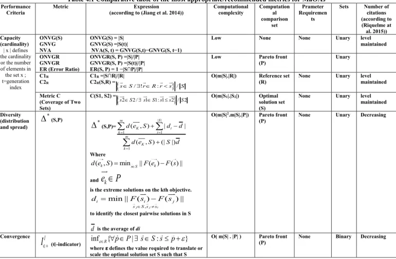
Table 4.1 Comparative table of the most appropriate/recommended metrics for MaOAs……….92
Table 4.2 Used objectives and their significance ………...…... 94
Table 4.3 Best, average and worst values of HV with non-correlated objectives, using 15 independent runs…..95
Table 4.4 Best, average and worst values of HV with correlated objectives using 15 independent runs………..95
Table 4.5 Best, average and worst HV with different population sizes and various objectives numbers………..95
Table 4.6 Average HV values with various scalarizing functions and correlation objectives relations……….…96
Table 4.7 Best, average and worst HV values using adaptive operators……….………97
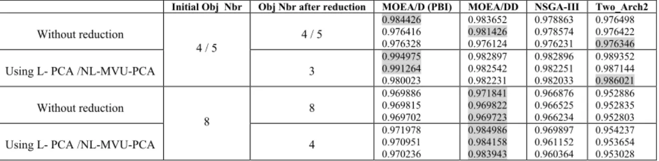
Table 4.8 Best, average and worst HV values before and after applying the dimensionality reduction…...98
Table 4.9 The correlation Matrix R on the first iteration………... 98
Table 4.10 The kernel Matrix K………...98
Table 4.11 Eigenvectors and eigenvalues of the matrix R………..………99
Table 4.12 Eigenvectors and eigenvalues of the matrix K……….………...99
Table 4.13 Eigenvalue Analysis for L-PCA ………..………99
Table 4.14 Eigenvalue Analysis for NL-MVU-PCA ……… ………99
Table 4.15 RCM analysis for L-PCA ………....….99
Table 4.16 RCM analysis for NL-MVU-PCA ………...………..….99
Table 4.17 Selection scheme for L-PCA ……….……….…..100
Table 4.18 Selection scheme for NL-MVU-PCA ………..………….100
Table 4.19 Median obtained solutions (objective values) ………...………...….100
Table 4.20 Median distance of the solutions obtained from the most preferred solutions……...………100
Table 4.21 Parameters setting of the algorithms………..…….101
Table 4.22 Hypervolume values (Best, average and worst)………… ……… ………101
Table 4.23 Average retained objective values………..….101
Table 4.24 Average distance between the most preferred solutions and the obtained ones……….102
Table 4.25 Features of the used DTLZ test problems………..……….102
Table 4.26 Best, average and worst IGD values on DTLZ1-4 problems……….……….103
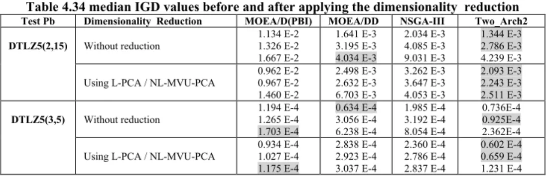
Table 4.27 Best, average and worst IGD values on DTLZ5(2,15) and DTLZ5(3,5) problems……...………….104
Table 4.28 Best, average and worst IGD values on DTLZ1 and DTLZ2 for different population sizes………..104
Table 4.29 Best, average and worst IGD on DTLZ(2,15) et DTLZ(3,5) for different population sizes…...……105
Table 4.30 IGD median values on DTLZ1 and DTLZ2 for different population sizes………106
Table 4.31 Median IGD on DTLZ1 and DTLZ2 using neighborhood mating and adaptive recombination..…..106
Table 4.32 Median IGD on DTLZ(2,15), DTLZ(3.15) with neighborhood mating, adaptive recombination...106
Table 4.33 Smallest non-redundant objectives number on DTLZ5(2,15), DTLZ5(3,5)………...107
Table 4.34 median IGD values before and after applying the dimensionality reduction………...…..108
Table 4.35 Median distance between the obtained solutions and the most preferred solutions for ds =0.01…...108
Table 4.36 Parameters of the experiments ………..……….…119
Table 4.37 Technical characteristics of the used TeensyWiNo nodes………..………120
Table 4.38 Technical and localization characteristics of the installed node………...…..122
Table 4.39 Locations of selected positions taken by the mobile node 'C'………...…..123
Table 4.40 The improvement of RSSI and FER rates compared to the initial deployment, by day……….126
Table 4.41 The improvement of RSSI and FER rates compared to the initial deployment, by night…….……..126
Table 4.42 HV (Best, average and worst values) ………..………..131
Table 4.43.Setting parameters of the algorithm………..……..134
Table 4.44. Hypervolume values (Best, average and worst) ………. ………..135
Table 4.45 Best, average and worst IGD values onDTLZ1-4 test suite………..……..136
acMaPSO accent-based Many-objective Particle Swarm Optimization
acMaMaPSO accent-based many-objective multi-agent Particle Swarm Optimization AcNSGA-III Ant colony NSGA-III
ACO Ant colony optimization
AGP Art Gallery Problem
AHCH Adaptive Hole Connected Healing
AI Artificial Intelligence
AIS Artificial Immune System
AmN Adaptive multi-Mutation strategy with Neighbourhood restrictions
AODV Ad-hoc On-demand Distance Vector
AxN Adaptive multi-Recombination with Neighbourhood restrictions
BCO Bees Colonies Optimization
BDA Bernoulli Deployment Algorithm
BDI Belief-Desire-Intention (model)
BS Base Station
CA Convergence Archive
cNSGA-III constrained NSGA-III
CSMA/CA Carrier-sense multiple access with collision avoidance
DA Diversity Archive
DAI Distributed Artificial Intelligence dBm Decibel-milliwatt (unit)
DDA Differentiated Deployment Algorithm DL-IoT Device Layer -Internet of Things
DM Decision Maker
DRP Dominance Relation Preservation-based
DSN Directional Sensor Networks
DTLZ Deb-Thiele-Laumanns-Zitzler (test problems)
DV-Hop Distance Vector Hop
EA Evolutionary Algorithm
EC-NSGA-II Extremized-Crowded NSGA-II
EMaO Evolutionary Many-objective Optimization EMO Evolutionary Multi-objective Optimization
EMOA Evolutionary Multi-objective Optimization Algorithm
FER Frame Error Rate
FS Feature Selection
GD Generational Distance
GNVG Generational Non-dominated Vector Generation GNVGR Generational Non-dominated Vector Generation Ratio
GPS Global Positioning System
GSM Global System for Mobile Communications
HV HyperVolume
IGD Inverted Generational Distance
IoT Internet of Things
JADE Java Agent DEvelopment framework
LoS Line of sight
LQI link quality indication
LoRa Long Range
LS Local Search
L-PCA Linear Principal Component Analysis MaOA Many-objective optimization Algorithm
MaOEA Many-objective Optimization Evolutionnary Algorithm MaOP Many-objective Optimization Problem
MaOPSO Many-objective Particle Swarm Optimization
MOEA/D Multi-objective Evolutionnary Algorithm based on Decomposition
MOEA/DD Multi-objective Evolutionnary Algorithm based on Decomposition and Dominance MOGA Multi-Objective Genetic Algorithm
MOP Multi-objective Optimization Problem MOPSO Multi-Objective Particle Swarm Optimization
MVU Maximum Variance Unfolding
NL-MVU-PCA Non-Linear-Maximum Variance Unfolding-Principal Component Analysis
NPGA Niched Pareto Genetic Algorithm
NSGA Non-dominated Sorting Genetic Algorithm
NU Network Utilization
NVA Non-dominated Vector Additional OMNeT++ Objective Modular Network++
ONVG Overall Non-dominated Vector Generation ONVGR Overall Non-dominated Vector Generation Ratio PAES Pareto Archived Evolutionary Strategy
PBI Penality-based Boundary Intersection
PCA Principal Component Analysis
PCS Pareto Corner Search based
PCSEA Pareto corner search evolutionary algorithm PESA Pareto Envelope-based Selection Algorithm
PF Pareto front
PFDA Potential Field Deployment Algorithm PI-EMOA Progressively Interactive EMO algorithm
PI-EMO-PC Progressive-Interactive-Evolutionary Multi-objective Optimization-Polyhedral Cone PI-EMO-PC-INK Progressive-Interactive-EMO- Polyhedral Cone-Ideal point-Nadir point-Knee points PI-EMO-VF Progressive-Interactive-Evolutionary Multi-objective Optimization-Value-Function
PL Path loss
PP Positioning Problem
PSO Particle Swarm Optimization
RCM Reduced Correlation Matrix
RERR Route Error
RoI Region Of Interest
RREP Route Reply
RREQ Route Request
RSSI Received Signal Strengh Indication
SA Simulated Annealing
SBX Simulated Binary Crossover
SMCP Set MultiCover Problem
SOP Single-objective Optimization Problem SPEA Strength Pareto Evolutionary Approach TCB Weighted Tchebycheff Distance TKR-NSGA-II Trade-off-based KR-NSGA-II
TS Taboo Search
Two_Arch2 Two_Arch2 Two-Archive2 (algorithm)
UASN Underwater Acoustic Sensor Network
UFS Unsupervised Feature Selection-based
USN Underwater Sensor Network
UWB Ultra Wide Band
U-NSGA-III Unified NSGA-III
VEGA Vector Evaluated Genetic Algorithm
VFA Virtual Force Algorithm
VP Voronoi Partition
WFG Walking Fish Group (test problems)
WiFi Wireless Fidelity
WiNo Wireless Node
WS Weighted Sum
WSN Wireless Sensor Network
Introduction and overview
Motivations and problematic
With different contexts of application, wireless sensor networks (WSN) are a research field that is in continuous evolution, especially with the emergence of the Internet of Things (IoT). Indeed, IoT is a concept that is closely related to the issues discussed in our study. IoT is a scenario in which different heterogeneous and communicating entities called objects or things (people, robots or devices) are connected and distinguished by unique identifiers. These entities can automatically transfer data to the network without any human intervention. WSN is the bridge connecting the real world to the digital one. It provides hardware communication to transmit and retrieve real values detected by wireless connected objects (sensor nodes). While the role of IoT is to process this data, manipulate it and make the decisions. In this thesis, we are interested in DL-IoT (DeviceLayer-IoT) networks which are collection networks used to collect data from distributed sensor nodes in the environment of the network. Hence, our approach can be applied for both WSN and IoT contexts. In this respect, given the limited energy, processing and memory capacity of sensors/objects, DL-IoT collection networks raise many optimization problems. Our global contribution is the proposal of heuristics, hybrid meta-heuristics (centralized and distributed), multi-objective models, mathematical formulations and evaluations of recent optimization approaches on DL-IoT collection networks. Given the continuous growth in the themes of DL-IoT collection networks, different contexts can be reversed such as optimizing the deployment of nodes. Deploying the nodes is the first step in installing a WSN. In terms of energy consumption optimization, this first step greatly affects the performance, reliability and operation of the network. The problem of deploying the nodes can be described as the positioning of all the sensors (that can be randomly scattered initially) constituting the network. To compensate their erratic nature of placement, a large number of sensors are often deployed intelligently. This can also contribute in increasing the fault tolerance of the network. For the 2D deployment of WSN, a very abundant literature exists ranging from the topological organization of the network to the technical specificities of the sensors and their way of communicating. However, the low-cost 3D deployment poses many optimization problems with a limited literature. Hence, our goal is to find the most optimized architecture and provide 3D sensor solutions, while improving the network performance. In this respect, several issues and objectives are related to the problem of deployment of sensor networks such as energy consumption, lifetime and localization. As a result, different heuristic approaches can be considered for optimizing WSNs.
The distributed and dynamic nature of the deployment problem requires the use of advanced and recent optimization and modeling methodologies: hybrid meta-heuristics. These latters allow exploiting the complementarity of these methods with each other and taking advantage from the benefits of other conventional approaches hybridized with them. This new class of hybrid meta-heuristics has shown its performance in solving difficult optimization problems especially when faced by objectives (like ours) that mainly concern the assurance of an evolutionary, flexible and robust system against network disturbances. Our contribution consists in putting a set of well justified modifications and hybridizations on the meta-heuristics, then applying them and evaluating their performances on our real world problem of deployment. In this respect, the most difficult optimization problems to be solved are generally derived from real problems that are often unmeasurable, complex and antagonistic.
In general, these problems include several criteria. This is due to the fact that they have several evaluation objectives; often contradictory; to be considered simultaneously. This gave birth to the theory of multi-objective optimization. In the literature, several methods of solving multi-objective problems have been developed. These methods can be classified into two main classes: exact methods and approximate ones that are subdivided into meta-heuristics and specific meta-heuristics. Meta-meta-heuristics form a set of optimization algorithms that aim to solve difficult optimization problems. These algorithms allows improving the quality of the solutions without guaranteeing the optimality of the obtained solution but in a very reasonable calculation time with respect to the complexity of the problem, often unsolvable in a polynomial time. Real-world optimization problems often have several conflicting and contradictory objectives and constraints (called multi-objective optimization problems (MOP)). This implies that there is not a single solution that is optimal in relation to all these objectives in the same time. The output of such multi-objective optimization algorithms is generally composed of a set of incomparable non-dominated solutions. These solutions are called "Pareto front" (PF). The goal of multi-objective optimization is to find a well-distributed and well-converged approximation of the PF. Subsequently, the decision maker (DM) can select the preferred solution. To determine the PF of a problem, various methods that are based on the imitation of the principles of biological evolution, have been proposed in the literature. These methods, named evolutionary algorithms (EA), have become popular and widely used in the resolution of MOPs because of their insensitivity to the objective function aspects and forms such as multimodality, discontinuity, convexity and its search space uniformity (Deb 2001). Indeed, evolutionary multi-objective optimization (EMO) is a new branch of optimization that has emerged following this success of the Multi-Objective Optimization EA (MOEA) on MOP resolving.
Research aims and principal contributions
The aim of this thesis is to propose hybridizations and modifications of evolutionary optimization algorithms in order to realize the adequate positioning of nodes in WSN while satisfying a set of constraints and objectives.
• As a first stage, an in-depth literature review was conducted on the methods of optimizing the deployment in WSN, especially the methods resolving the 3D indoor deployment. This study covers swarm-based meta-heuristics (particle swarm optimization, ant colony optimization and bee hives algorithm), genetic algorithms, taboo research and simulated annealing. The study also deals with the single-objective and multi-objective case; the static and dynamic case; the distributed and parallel case of deployment.
• In the second stage, a mathematical formulation based on an Integer Linear Programming model and aims at modeling the problematic is proposed. This formulation identifies and explains the objective function to optimize, the decision variables and the different constraints to be taken into consideration. Our goal is to minimize the number of sensor nodes to use and the energy consumption. At the same time, maximizing the network lifetime, the coverage, the localization and connectivity. • In the third stage, the focus is on the proposition of different justified hybridization and modifications schemes introduced on the optimization algorithms in order to better solve the deployment problem:
- In a first approach, an adaptive mutation and recombination operators with neighborhood mating constraints are proposed. The use of a concept of multiple scalarization functions is introduced to deal with: (i) the inefficiency of Pareto-based multi-objective evolutionary algorithms, (ii) the inefficiency of the
recombination operation, and (iii) the exponential increase in costs (time and space) when solving multi-objective problems in the real world context.
- In a second approach, the incorporation of preferences is established: In the case of real world problems having a large number of objectives, the size of the population and the number of necessary solutions depend exponentially on number of objectives. Thus, the performance of the optimization algorithms deteriorates when solving such problems. To solve this challenge, the NSGA-III algorithm is hybridized with an interactive user preference strategy (PI-EMO-VF) that follows the evolution of new solutions to gradually incorporate the preferences of the user. In this work, the effectiveness of the NSGA-III is tested in real-world problems, and compared to another recent multi-objective algorithm (MOEA/DD).
- In a third approach, a justified hybridization scheme that combines three classes of multi-objective algorithms. These algorithms rely on reference points (NSGA-III, MOEA/DD), aggregation (Two_Arch2) and decomposition (MOEA/D) with two procedures based on dimensionality reduction (MVU-PCA) and preferences (PI-EMO-PC). The purpose of this hybridization is to benefit from the advantages of each method to solve our complex problem.
- In a fourth approach, a new hybrid algorithm derived from biological observations (ant search behavior and genetics) is proposed. It is based on the recent variant of the genetic algorithms (NSGA-III) and the ant colony algorithm (ACO). This is the first time NSGA-III and ACO are integrated into a hybrid platform. Moreover, unlike traditional hybridizations, these two algorithms iterate at the same time and interact using the same population (the initial population of the NSGA-III is the population built by the ants in the initial phase of the ACO in the same iteration). Then, the steps of the ant algorithm are injected into the NSGA-III with incorporation of several modifications on the original NSGA-III.
- In a fifth approach, a particle swarm optimization algorithm (called acMaPSO) based on a new bird accent concept is proposed. The new bird accent concept relies on a set of birds that are separated into different accent groups by their regional dwelling and are classified into groups according to their ways of singing. This new concept of bird accent is introduced to preserve the diversity of the population during research and to assess the particle search capability in their local areas. To ensure that the search escapes local optima, the most expert particles (the parents) "die" and are regularly replaced by new particles that are randomly generated.
It is also proposed to test this hybridization in a distributed environment. For this purpose, it is proposed to hybridize the acMaPSO algorithm with a multi-agent system (MAS). The new variant (named acMaMaPSO) takes advantage of agent distribution and particle interactivity. We propose a decentralized multi-agent architecture that contains three types of agents: an environment agent, swarm agents and bird agents (or particle agents). These agents have different knowledge, goals, abilities and action plans.
All these proposed hybridizations are tested and approved by numerical results that use evaluation metrics such as the Hypervolume. Afterwards, simulations and prototypes on real testbeds have been proposed. Then, in order to prove the stability and efficiency of these hybridizations in different contexts, the simulations are confronted with real experiments.
Structuring of the document
This document is structured into four chapters divided in two parts. The first part illustrates the state of the art in the first two chapters; and the second part details the proposed contributions in chapters 3 and 4.
The first chapter starts by presenting the state of the art of the 3D indoor deployment problem. We introduce the issues of the three-dimensional deployment and its different types, objectives, models and applications. Then we identified and criticized the recent research works dealing with the problem of deployment.
The second chapter introduces the methods used to solve the 3D indoor deployment, especially the evolutionary optimization algorithms, the multi-agent systems and the incorporation of dimensionality reduction and user preferences. We also detail the fundamental concepts of multi-objective optimization such as the dominance and the Pareto front. Then we describe the main classical approaches and meta-heuristic of resolution of multi-objective problems.
In the third chapter is dedicated to illustrate our mathematical modeling of the deployment problem based on an integer linear programming formulation. We present the architecture of nodes, the assumptions, the notation and the objective function. Then we detail the considered objectives and their specificities. Moreover, this chapter is devoted to explain and justify the proposed hybridizations and modifications that are introduced to meta-heuristics to improve their performances and capabilities to solve optimization problems. Especially complex and many-objective real world problems like ours. These changes relies essentially on the following contributions: the use of the neighborhood and adaptive recombination operators; the use of multiple scalarizing functions in the aggregation based approach; the incorporation of dimensionality reduction and users preferences; a hybrid framework for NSGA -III and Ant system; and finally the proposition of a concept of bird accents in PSO and its hybridization with MAS.
The last fourth chapter is devoted to illustrate the results of various evaluations. We initially introduced the different test parameters and evaluation metrics that we used to validate our proposals. We turn next to illustrate the numerical results of the 3D deployment problem after incorporating our proposed hybrid scheme of dimensionality reduction and preferences. Then we present the results on the DTLZ unconstrained test functions. Afterward, we propose a study that investigates the modeling of the used protocols and presents the simulations with small and large instances. Next, we propose ACO and NSGA-III experiments, then the results of the based-on bird’s accent PSO algorithm and the PSO-MAS one.
Finally, we present our conclusions as well as our perspectives and futures directions of research.
Part I
Chapter 1
The 3D indoor deployment problem in WSN and DL-IoT
collection networks
1.1 Introduction ...7
1.2 Presentation, migration from WSN to DL-IoT and complexity of the deployment problem ...7
1.3 The 3D deployment strategies in WSN ...10
1.3.1 Full coverage ... 10
1.3.2 K-coverage ... 11
1.3.3 Surface coverage ... 11
1.4 Conflicting types of deployments ...11
1.4.1 Single Objective deployment vs. multi-objective deployment ... 11
1.4.2 Deterministic deployment vs. stochastic deployment ... 12
1.4.3 Stationnary deployment vs. mobile deployment ... 12
1.4.4 Homogenous deployment vs. heterogeneous deployment ... 12
1.4.5 Static deployment vs. dynamic deployment ... 13
1.5 Initial objectives to be satisfied during deployment ...13
1.5.1 The number of deployed nodes, cost and scalability ... 13
1.5.2 Coverage problem ... 14
1.5.3 Connectivity problem ... 15
1.5.4 Coverage with Connectivity ... 16
1.5.5 Energy efficiency ... 16
1.5.6 Network lifetime ... 17
1.5.7 Network traffic... 17
1.5.8 Data fidelity ... 17
1.5.9 Fault tolerance and load balancing ... 18
1.5.10 Latency ... 18
1.6 Sensing models ...18
1.6.1 Binary model ... 18
1.6.2 Probability model ... 19
1.6.3 Tracking detection model ... 19
1.6.4 Coverage and connectivity model ... 20
1.7 Open deployment issues ...20
1.8 Applications of the deployment ...23
1.9 Methodologies for solving the problem of deployment ...25
1.9.1 Virtual Force algorithms ... 26
1.9.2 BDA, PFDA and DDA Algorithms ... 26
1.9.3 Heuristic optimization ... 26
1.10 Other problems similar to the node positioning problem ...26
1.10.1 Set MultiCover Problem ... 26
1.10.2 Art Gallery Problem ... 27
1.10.3 Other similar problems ... 27
1.11 Comparaison and review of recent studies on WSN deployment ...27
1.1 Introduction
Deployment represents a fundamental role in setting up efficient wireless sensor networks (WSN). In general, WSN are widely used in a variety of applications ranging from monitoring a smart house (planned deployment) to monitoring forest fires with parachuted sensors (random deployment). In this first chapter, we focus on the planned deployment, in which the sensor nodes must be accurately positioned at predetermined locations to optimize one or more design objectives of the WSN, under some given constraints. The purpose of planned deployment is to determine the type, number, and locations of nodes to optimize coverage, connectivity and network lifetime. There have been a large number of studies, which proposed algorithms for solving the premeditated deployment problem. The main purposes of this chapter are two-fold. The first one is to present the complexity of 3D deployment and then detail the types of sensors, objectives, applications and recent research that concerns the strategy used to solve this problem. The second one is to present a comparative survey between recent optimization approaches used to resolve the deployment problem in WSN. Based on our extensive review, we discuss the strengths and limitations of each proposed solutions and compare them in terms of the different WSN design factors.
1.2 Presentation, migration from WSN to DL-IoT and complexity of the
deployment problem
Another concept is closely related to our problem, it is the IoT (Internet of Things). The IoT is a scenario in which entities (devices, people or robots) are connected and have a unique identifier for each. They are able to transfer data over the network without human or automatic intervention. These objects communicate using protocols such as the Bluetooth or the 802.15.4 as it is the case in our experiments (section 4.5). WSN is the bridge which links the real world to the digital one. It is responsible for the hardware communication to convey the real world values detected by the wireless connected things (sensor nodes) to the Internet. While the IoT is responsible for data processing, manipulation and decision making. In our study we are interested in the DL-IoT (DeviceLayer-IoT) (Van den Bossche et al, 2016) which is a network of collection used to collect data from the sensors nodes disseminated in the network environment. Thus, our approach and contributions are valid for both WSN and IoT contexts.
Indeed, a fundamental problem in the WSN is how to deploy sensor nodes. The deployment problem can be described as follows: Having N wireless sensors and an area A to cover, how to deploy these sensors to form a WSN that meets system requirements, such as the connectivity of the network, its ability to detect relevant events happening in A, and its ability to provide a required period of operation. This problem is related to coverage, connectivity, and lifetime issues. Indeed, the problem of deployment in WSN refers to the determination of the positions of nodes (and/or the base stations) so that the coverage, the connectivity and the energy efficiency can be obtained with a minimum number of nodes.
Events happening in an area lacking a sufficient number of nodes may be unnoticed. Moreover, areas with dense sensor populations suffer from congestion, redundancy detection, and delays. Optimal deployment ensures adequate quality of service, long network life and cost saving. The problem of deployment can also be defined as follows: having a surface A in 2D or 3D with a set of obstacles (if these obstacles exist, they should not partitionate A) and a set of sensors with different types (according to their radii of detection and communication), the overall goal is to minimize the number of nodes to be deployed on A while ensuring one or more objectives such as network coverage and connectivity. It is said that the target region is covered if each point in A is covered by an active sensor having a probability of coverage Pc and a sensing range Rs if there is direct communication (Line of Sight). Besides, it is said
that the network monitoring a target region is fully connected if all sensors can route data in multi-hop to the base station or to another destination node.
Most deployment approaches consider a WSN with randomly deployed sensors (Ammari, 2014) which are generally modeled by a Poisson point process with a density γ. This Poisson process is defined as follows: for any zone A in the region R, the distribution of the number of nodes in A is the mean distribution of Poisson γ‖A‖, ‖A‖ is the surface of A (Ammari, 2014). Given the number of nodes, their locations are mutually independent random variables and uniformly distributed over A. It is known that n nodes whose locations are mutually independent random variables, with a uniform distribution within A, are mainly associated to a Poisson process with a density γ, provided that A is large (Hall, 1988).
An example of randomly deployed sensor networks is shown in Figure 1.1. There are twelve sensors deployed in a rectangular detection field. The density of sensors on the left side of the field is higher than that on the right one. Therefore, the detection field is not fully covered by the sensors.
Figure 1.1 An example of area coverage using randomly deployed sensors
Finding the optimal node distribution is a difficult problem to solve and is considered NP-hard for most formulations. This problem is proven to be optimally solved in 2D environments while it has been proven to be NP-difficult if it is generalized to 3D environments (Cheng et al., 2008). Figure 1.2 shows an example of 2D deployment and another for 3D deployment.
2D deployment 3D deployment
Figure 1.2 The 2D deployment vs. the 3D deployment
When sensors are deployed randomly, the initial coverage area provided by the network cannot be optimal as in the case of deterministic deployment. In order to increase the covered area, redundant sensors are deployed. Redundancy makes sensor networks denser than normal ad hoc networks. However, increasing sensor density cannot provide a 100% coverage probability. In addition, it is expensive to maintain high-density WSN on a large scale. Therefore, other approaches should be used to avoid these problems and improve the
coverage after the initial random deployment. Another problem that complicates the redeployment is that of the robustness of WSN. Indeed, once deployed, it is expensive and impractical, even impossible, to replace unusable sensors in most types of applications. Hence, if a particular node is no longer running, there will be an impact on the overall performance of the network. The loss of a node may be due to different causes, such as battery depletion, physical damage caused by environmental forces, or destruction by the enemy. If a sensor that covers a sensitive area dies and no other sensor can cover that area, the WSN fails its mission of efficiently distributing the sensors.
Indeed, one way to optimize the distribution strategy in WSN is to have redundant sensors that improve the performance of the network. In addition, if the detection field is vast or has limited access, the sensors may not be able to be deployed one by one in specific locations. Instead, they can be disseminated from an airplane. When the sensors are randomly deployed, the initial coverage area provided by the network cannot be optimal as in the case of deterministic deployment. In order to increase the coverage area, redundant sensors can be deployed. Redundancy makes sensor networks denser than ad hoc networks. However, increasing sensor density can not provide a 100% coverage probability. Even more, it is expensive to maintain high-density sensor arrays on a large scale. Therefore, other approaches should be used in order to avoid these problems and improve the coverage after the initial random deployment. Another problem that complicates the redeployment is the robustness of WSN. Once deployed, it is expensive and impractical, if not impossible, to replace unusable sensors in most types of applications. Therefore, if a particular node is no longer running, there will be an impact on the overall performance of the network. The loss of a node may be due to various causes such as battery depletion, physical damage from environmental forces, or destruction by the enemy. If a sensor that covers a sensitive area dies and no other sensor can cover that area, the sensor array fails in its mission of efficiently distributing the sensors.
The process of deploying sensor nodes greatly influences the performance of a WSN. The problem of deployment or positioning nodes in a WSN is a strategy that defines the topology of the network, and therefore the number and position of nodes. The quality of monitoring, connectivity, and power consumption are also directly affected by the network topology.
The different deployment tasks can be grouped into three main phases: A pre-deployment and pre-deployment phase (Figure 1.3 (a)) which is achieved by the manual placement of nodes or the spreading of nodes from a helicopter, for example. A phase of post-deployment (figure 1.3 (b)) is necessary if the topology of the network has evolved, for example following a displacement of nodes, or a change of the radio propagation conditions. The third phase concerns the redeployment (Figure 1.3 (c)) which is based on adding new nodes to the network in order to replace some failed nodes. The system can iterate on phases 2 and 3.
(a) Pre-deployment and deployment phase
(c) Redeployment phase Figure 1.3 Phases of deployment
Different issues are encountered at the level of the deployment of sensor nodes in WSN. These studies mainly concern stationary and mobile cases; single and multi-objective cases; deterministic and stochastic aspects; and finally static and dynamic deployments.
The coverage is affected by the sensitivity of the sensors represented by the detection range (noted Rs), while the connectivity is guaranteed by the communication range (noted Rc). According to (Frye et al., 2006), the degradation of the coverage probability in some
WSN applications is tolerable, whereas the degradation of the probability of connectivity could be fatal for the network. In the context of dynamic deployment, we investigate in (Mnasri et al., 2014a) the research works proposing solutions for the sensor nodes repositioning and its related issues. Connectivity and coverage are the most used factors in determining the communication and the detection efficiency, respectively. Moreover, we propose in (Mnasri et al., 2014a) and (Mnasri et al., 2014b) a detailed study of deployment in the static case. They distinguish two deployment methodologies according to the distribution of the nodes (either random or controlled). The treated primary objectives can be as follows: - The coverage which is one of the most preponderant problems in WSN. Several types of coverage are presented: point coverage, area coverage, barrier coverage and coverage of an event or a moving target.
- The consumed energy and ensuring the energy efficiency. - The network connectivity.
- The lifetime of the network. - The network traffic.
- The reliability of data.
- The cost of deployment (depending on the number of deployed nodes). - The fault tolerance and load balancing between nodes.
1.3 The 3D deployment strategies in WSN
When designing deployment strategies, several factors must be considered such as the monitoring area, the sensor capabilities (detection range and transmission range), the area coverage, and the lifetime. The following questions should also be considered when establishing a deployment strategy: how many sensors should be deployed? How to place sensors in the monitoring area? Where to put the sink if we can choose its position? The number of sensors can be deduced from the lower limit of the monitoring area, sensor capacity and design requirements. Three types of coverage exist:
1.3.1 Full coverage
Full coverage is achieved if every point in the 3D RoI is at least covered by a sensor. Full area coverage requires the deployment of a large number of sensors, which increases cost and complexity. However, partial coverage only guarantees a certain percentage of coverage (Wang et al., 2007). Figure 1.4 illustrates different geometric layouts used in the 3D coverage.
Figure 1.4 Different geometric 3D coverage layouts (Younis and akkaya, 2008)
1.3.2 K-coverage
With regard to the k-coverage, a 3D RoI is assumed to be k-covered if there are at least k sensors that cover and monitor each point of the 3D RoI. Indeed, k-coverage represents the logical extension of the case of 1-coverage. In the case of k-coverage, the distance between the detection nodes is minimized with the appearance of overlaps between the detection spheres. In general, when achieving the k-coverage optimally (K>1), the complexity of the coverage algorithm will increase (Xu et al., 2010).
1.3.3 Surface coverage
In the case of surface coverage (shown in Figure 1.5), the sensors can only be deployed on the surface of the RoI. Many real applications require this kind of surface coverage where the RoI is a complex surface that is neither a complete 3D space nor a 2D plane. Mathematically, the detection field can be modeled as several small simplified rectangles as a single-valued function z=f(x, y) with two node distribution models: a planar surface Poisson point model and a space surface Poisson point one (Ammari, 2014). (Jin et al., 2012) addresses the problem of surface coverage in terms of reliability of the monitored data and quality of detection.
Figure 1.5 3D surface coverage (Ammari, 2014)
1.4 Conflicting types of deployments
1.4.1 Single Objective deployment vs. multi-objective deployment
The criteria and objectives, on which the deployment is optimized, are often contradictory. This is the case of coverage and energy consumption because the best the coverage is, the most the energy consumption is. It is also the case of the survivability and fault tolerance. Therefore, we cannot find a deployment that optimizes all objectives simultaneously. Hence the need for an optimal trade-off between the different objectives. According to the used approach, we can either optimize each objective alone or use an aggregation function that combines all objectives in a single function with weights that represent the importance of each objective.
1.4.2 Deterministic deployment vs. stochastic deployment
When the selection of sensor positions is possible and determined beforehand, this is referred to as the deterministic deployment. When sensors can be dropped from an aircraft, for example, this is referred to as the non-deterministic or stochastic deployment. This last type of deployment cannot be optimal as long as it can result in very dense areas and others less dense or even disconnected. Deterministic deployment provides an optimal network configuration. However, because of the size and density required to provide adequate network coverage across large geographic areas, careful node positioning is not practical. In addition, many WSN applications should operate in hostile environments which make the deterministic deployment impossible in some cases. As a result, stochastic deployment becomes the only possible alternative. As an example, the work of (Clouqueur et al., 2002) aims to determine the number of needed randomly deployed nodes for target detection by optimizing the deployment cost and the area coverage.
1.4.3 Stationnary deployment vs. mobile deployment
Considering the mobility of nodes as a criterion, two deployment strategies can be distinguished: static deployment in which nodes have unchanged positions and mobile deployment where the nodes have a mobile capacity and can move and reposition themselves after the initial deployment. Then, some regions of the network may become uncovered due to occurred events in the RoI or depletion of sensor batteries. A solution to remedy this is to move some mobile nodes to these regions. Various examples of mobile node applications can be cited such as target tracking, rescue or underwater and military surveillance. (Romer and Mattern, 2004) classify nodes according to their mobility into three classes: static nodes, mobile ones and mobile sinks. Figure 1.6 describes other characteristics of mobility: passive nodes are often attached to or carried by moving entities while active nodes have automotive capabilities. Besides, the degree of mobility varies from a continuous movement to an occasional movement with long periods of immobility.
Figure 1.6 Mobility taxonomy
However, differents studies (Idoudi et al. 2012), Idoudi (2017) highlights the necessity to optimize the movement of nodes. According to (Guvensan and Yavuz, 2011), moving a node one meter can consume more than 30 times of energy than transmitting 1 ko of data. Despite this, mobility provides better coverage and connectivity and increases the network adaptability.
1.4.4 Homogenous deployment vs. heterogeneous deployment
The type of application for which the WSN is installed determines the types of sensors to deploy: are they homogeneous or having different roles thus characterizing a heterogeneous architecture. A wireless network is qualified as heterogeneous if the distribution of the nodes in the RoI is heterogeneous. Indeed, the first visions of the WSN consider homogeneous devices, generally identical from software and hardware point of view. However, different recent applications require a variety of devices that differ in number, type and role played in
the network (some nodes may function as cluster heads or gateways to other communication networks such as GSM networks, satellite ones, LoRa, SigFox, 5G, NB-IoT or WiFi).
1.4.5 Static deployment vs. dynamic deployment
Static deployment assumes that there is no mobility after the first positioning of nodes in the network. In the case of static deployment, the best node locations are chosen based on the optimization strategy, then no changes will occur during the lifetime of the network. Static deployment can be either random or deterministic. As we mentioned before, the positions of nodes have a considerable influence on the performance of the WSN and its operation. On the other hand, metrics which are independent of the state of the network and assuming a fixed operation scheme are often used to choose the locations of nodes. Among these static metrics, the distance between nodes. Moreover, the initial configuration of the network does not take into account the dynamic changes during the operation of the latter such as the mobility of targets. Hence the interest of dynamically repositioning nodes during the network operation. For example, to substitute some nodes having exhausted batteries, other sensors can be moved. Dynamic deployment is a solution for the problem of no guarantee of optimality during the initial deployment. It assumes that nodes can move in a coordinated way in the RoI. However, the relocation of nodes during the network operation is often expensive and requires the continuous monitoring of the state of the network and the events occurring in the neighborhood of the node. In addition, solutions must be found to the problem of data manipulation and delivery during the relocation process.
1.5 Initial objectives to be satisfied during deployment
1.5.1 The number of deployed nodes, cost and scalability- Number of nodes: More than half of the papers dedicated to resolve the optimal deployment of nodes aim to reach the defined goals with a minimum cost. These studies are based on the assumption that low-cost detection devices embedded inside the sensors are used to monitor phenomena such as temperature, pressure, humidity, light, sound or magnetism. However, if we consider the deployment of hundreds or thousands of sensors, the overall cost of deploying the network must be taken into consideration. Thus, the number of sensors deployed is one of the essential measures that must be taken into account in the WSN deployment process. Indeed, in some specific applications, it is not realistic to consider low cost sensors because the more sensors used, the higher the cost becomes. Hence, the cost of a sensor strongly depends on the target application and the monitoring environment. For example, in the case of oceanographic applications such as offshore exploration, the cost of the sensor will be much higher because the detection device is much more sophisticated in order to detect specific phenomena and withstand the influences of the environment.
- Cost: The cost of a WSN starts from the construction phase of nodes. This cost may be variable depending on the application and the included detection devices. Nodes can be equipped with other equipment such as GPS that can increase the final cost of the node. Some applications do not take into account the cost of the node because of the low price of the used nodes. In this case, random deployment is an excellent way to deploy nodes in the RoI. A forest, an ocean or a battlefield are some examples of these applications. In other applications, the node costs are quite high and must be included in the node deployment strategies. Besides the node construction cost, deployment and maintenance costs are also applied to the total cost of a network. When the deployment is not random and is done by hand or with the help of particular automated robots, the cost of placing nodes must be taken into account. Indeed, the more the network needs nodes, the more its construction, deployment and maintenance will be high.