The effects of geometrical imperfections on the ultimate strength of aluminium stiffened plates subject to combined uniaxial compression and lateral pressure

(1)

The effects of geometrical imperfections on the ultimate strength of

aluminium stiffened plates subject to combined uniaxial compression and

lateral pressure

Mohammad Reza Khedmatia, Masoud Pedrama and Philippe Rigob

a

Faculty of Marine Technology, Amirkabir University of Technology, Tehran, Iran b

ANAST, University of Liège, Liège, Belgium

The present study aims at determining the effects of the geometrical imperfections on the ultimate strength and load-carrying capacity of aluminium stiffened plates under combined axial compression and lateral pressure. The finite element models proposed by the Committee III. 1 'Ultimate Strength' of ISSC'2003 are used in the present investigation. Initial imperfections as proposed by ISSC committee as well as those recommended by Ship Structure Committee are considered in the analyses. Models are tested using non-linear finite element elastic-plastic analyses. Aluminium alloy AA6082-T6 is selected as the material for the models. The studied models are triple-span panels stiffened by either extruded or non-extruded angle-bar profiles. Different arrangements of heat-affected zone (HAZ) are considered. The main outcomes of this study show the need for a subtle assessment of the real shapes of the initial deformations. The way they affect the ultimate strength of models is clarified through finite element analyses.

Keywords : aluminium stiffened plate ; initial imperfection ; ultimate strength ; finite element analysis ; heat-affected zone

Nomenclature

a Distance between transverse frames

b Distance between longitudinal stiffeners

B Overall width of the panel

E Young's modulus

hw Height o f stiffeners

L Overall length of the panel

t Plate thickness

U Displacement along x-axis

V Displacement along y-axis

W Displacement along z-axis

Wopl Buckling type initial deflection of the plating between stiffeners

Wopl* Maximum buckling type initial deflection of the plating between stiffeners

Woc Column-type deflection of the stiffeners

Woc* Maximum column-type deflection of the stiffeners

Wos Sideway initial deflection of the stiffeners

Wos* Maximum sideway initial deflection of the stiffeners

Slenderness parameter of the plate

ε Average strain

εult Average strain at ultimate strength stage

Column slenderness parameter of the stiffened plate

v Poisson 's ratio

σY Yielding stress

σiy Initial yielding stress

σ Average stress

σu Average stress at ultimate strength stage

σΥΗΑΖ Yielding stress of the heat-affected zone

θx Rotation about x-axis

θy Rotation about y-axis

(2)

1. Introduction

Stiffened plates are used as main supporting members in many civil and marine structural applications. They normally consist of a plate with equally spaced stiffeners welded on one side, often with intermediate transverse stiffeners or bulkheads. The most regular stiffener cross-sections are bulb, flat bar or T- and L-sections. Such structural arrangements are common for both steel and aluminium structures.

Aluminium panels were implemented for marine applications, such as construction of boats and high-speed catamarans, during 1990s for the first time (Collette 2005). The main role of these panels is to strengthen against in-plane compression. Ultimate strength formulations used for steel panels could not be directly applied for estimating the ultimate strength of aluminium panels. This is because the constitutive stress-strain relationship of the aluminium alloys is different from that of structural steel. In the elastic-plastic range after the proportional limit as compared to structural steel, the strain hardening has a significant influence in the ultimate load

behaviour of aluminium structures, whereas in steel structures, the elastic-perfectly plastic material model is well adopted. Besides, the softening in the heat-affected zone (HAZ) significantly affects the ultimate strength behaviour of aluminium structures, whereas its effect on steel structures is of very little importance (Khed-mati et al. 2009).

Investigations in aluminium structures are not as extensive as in steel structures. For example, Paik and Thayamballi (2006) summarised some of the remarkable developments related to the ULS design technology used in designing ship and ship-shaped offshore steel structures. They took into account some of the most important remarks in constructing marine structures such as stiffened panels, corrugated panels, ship hulls, fabrication-related initial imperfections, corrosion, fatigue cracking and local damage. The need for such investigations in aluminium structures is felt too.

Clarck's tests (Clarke and Narayanan 1987) were one of the first investigations done for aluminium panels. Eight different welded panels were included. Flat and T-bars were used as stiffeners. One of the largest and most relevant experimental programmes into the compressive collapse of aluminium structures is a series of 76 plate compressive collapse tests carried out by Mofflin (Collette 2005). This test investigated two most typical alloys for high-speed vessel construction: the 5083 and 6082 series. The tests were especially conducted to clarify the influence of out-of-plane deflection, longitudinal welds and transverse welds separately. Aalberg et al. (2001) conducted a similar test on extruded aluminium panels. The test panels consisted of single-span AA6082-T6 stiffened panels, with either open L-shaped or closed trapezoidal-shaped stiffeners. Zha and Moan (2001) and Zha (2003) carried out a series of compression tests on ship-type aluminium panels. The experimental

programme investigated 25 flat-bar stiffened panels, sized so that tripping of the stiffeners was the main failure mode. The panels were constructed out of AA5083-H116 and AA6082-T6 alloys, and were constructed by welding. The boundary conditions were simply supported at transverse ends and free longitudinal sides. Hopperstad et al. (1997) tested stiffened plates in compression, and compared the results with non-linear finite element predictions developed using the ABAQUS commercial code with good agreement. They also compared Mofflin's experimental plate tests with ABAQUS results and again observed good agreement. Herrington and Latorre (1998) carried out experimental and numerical studies on an aluminium panel with floating frame. Such a construction procedure proved to be efficient under the action of lateral pressure. Kristensen and Moan (1999) investigated the response of un-stiffened simply-supported aluminium plates with ABAQUS commercial codes, examining axial compression, biaxial compression, shear and combined load cases. They examined several different alloys and also studied the effect of HAZ by considering various HAZ locations and widths. Rigo et al. (2003) outlined a sensitivity study on the ultimate strength of aluminium panel based on a benchmark study carried out for the Committee III.1 'Ultimate Strength' of ISSC'2003. The extrusion cross-section, same as in Aalberg et al.'s experimental investigation, was selected and several finite element codes were compared to study the compression collapse and a good agreement observed between the results. However, a sensitivity study was held to study the effects of the HAZ extent, the locations of the HAZ including transverse welds at mid span, residual stresses, initial out-of-plane deformations and material properties. The most significant factors were the location and size of the HAZ, especially transverse weld lines, with the other factors having lesser impact on the ultimate strength.

In two series of tests supported by the Ship Structure Committee, Paik et al. built 78 welded aluminium panels taking into account a high-speed vessel structure (Paik et al. 2008, Paik 2009). The panels were studied and several empirical formulas developed based on these observations and using statistical methods. Further investigations were carried out on panels to determine their ultimate strength and collapse mode. Investigations included welded panels using MIG and FSW methods. Furthermore, recommendations were made for finite element analysis of the panels. Finally, the computational and experimental results were compared with each

(3)

other and good agreements between them were observed.

Sielski (2008) established a roadmap for researchers by outlining the future trends and research needs in aluminium structures. These researches necessitated studies in areas such as material property and behaviour, structural design, structural details, welding and fabrication, joining aluminium to steel, residual stresses and distortion, fatigue design and analysis, fire protection, vibration, maintenance and repair, mitigating slam loads and emerging technologies. Further development of finite element investigations has accelerated the

investigations in the field of buckling and ultimate strength of different structures by conducting elastic-plastic large deflection analyses (Kim et al. 2009). Khedmati et al. (2009) investigated the effect of thickness of plating, changes in stiffener profiles and dimensions on the ultimate strength and buckling behaviour of an aluminium panel. Initial imperfections due to welding were also considered in their investigations. Khedmati and Ghavami (2009), taking into account the shortcomings in the investigations of panels with fixed/floating stiffeners, set up a series of finite element investigations in order to find the advantages and disadvantages of stiffening method. Lattore's panel and four similar panels in dimension were analysed using a nonlinear finite element method. Khedmati et al. (2010), in continuation with investigations done by Committee III.1 'Ultimate Strength' of ISSC'2003, selected the Committee's proposed models and analysed them under axial compression and lateral pressure. Furthermore, Benson et al. (2011 ), using a non-linear finite element approach, examined the strength of a series of unstiffened aluminium plates with material and geometric parameters typical for the midship scantlings of a high-speed vessel. Based on some parametric studies, they proved that geometrical and material factors have a significant influence on the strength behaviour of the plates before and after collapse point. From the investigations of aluminium strength, it is understood that several different methods have been used in modelling the welding-induced initial imperfections, especially in finite element investigations. In most of the investigations, the observations from experimental studies have been implemented. Two major and most

implemented methods are Park's empirical formulations and Rigo's proposed procedure in modelling geometrical imperfections. In the present study, the finite element models proposed by ISSC'2003 are selected. Aluminium alloy AA6082-T6 is the material used for these panels. The above-mentioned procedures are implemented on models and tested under combined loading condition of in-plane compression and lateral pressure using non-linear finite element analysis. Finally, the results of models of two types of imperfections are compared and proper conclusions are made.

(4)

2. Models for analysis

2.1. Structural arrangements and geometrical characteristics

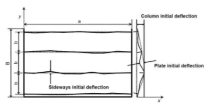
Rigo et al. (2003) considered a three-span plate with L-shaped stiffeners fabricated from aluminium profiles, joined by welding, for the finite element analyses. This model is also selected for the present study. Figure 1 illustrates the geometrical specification of the model with the XYZ coordinate system and the U-V-W

corresponding displacements. Rigo et al. (2003) performed a detailed benchmark study on the ultimate strength of stiffened aluminium plates under in-plane compression. They introduced this model as an appropriate model for conducting finite element investigations with reliable results when studying the behaviour of axially compressed aluminium stiffened plates.

2.2. Finite element code and adopted elements

All analyses in this study are carried out using the commercial finite element code ANSYS. The SHELL181 element from the programme element library is selected in order to discrete the stiffened plate models.

SHELL181 is well suited to model moderately thick shell structures. The element has six degrees-of-freedom at each node: translations in the nodal x, y and z directions and rotations about the nodal x, y and z axes. The element has plasticity, vis-coelasticity, stress stiffening, element birth and death, large deflection and large strain capabilities (ANSYS 2007).

2.3. Mechanical properties of material

Models are in aluminium alloy AA6082 temper T6, where its stress-strain curve is selected based on

experimental results of Aalberg et al. (2001). The stress-strain curve of this alloy is represented in Figure 2. The mechanical properties of this alloy are presented in Table 1.

Figure 2. Average stress-average strain curve of the aluminium material in standard state and also in HAZ.

(This figure is available in colour online.)

2.4. Boundary and loading condition

In the present study, as proposed by Rigo et al. (2003), along the longitudinal edges (unloaded), the assumed boundary conditions of the stiffened plates are simply supported which are kept straight (constrained edges). The loaded edges are restrained from rotation, and an axial displacement is prescribed (W = V = 0 and restrained rotation θy = 0, with U = 0 on one side and U = U* on the other side). At two loaded edges, because of stiff

transverse frames, the cross-sections remain plane. One should note that the two end frames (T1 and T4) are assumed perfectly rigid (Figure 1). Their dimensions are 1262.5 × 71.8 mm2 and thickness 10 mm.

Table 1. Mechanical properties of the material.

E (MPa) v σY(MPa)

(5)

Figure 3. Boundary conditions of the model. (This figure is available in colour online.)

There are T2 and T3 frames with thickness of 3 mm at the intermediate support locations (Figure 1). These two intermediate and the two end frames provide support for the five longitudinal and the sideways deformation of the stiffeners not being allowed. This means that V is restrained at four points in the main plate, along the symmetry axis (Figure 3). Furthermore, unloaded longitudinal edges remain straight (V remains constant along these two edges). Due to presence of stiff transverse frames, the displacements (W) along Z of these two end transverse plates are not allowed. W = 0 is assumed for all the nodes at the intersection between the main plate and the two end transverse support plates (Figure 3).

In case of pure in-plane compression, uniform in-plane displacement is imposed on one of the loaded edges while the other loaded edge is restrained against in-plane movement. When lateral pressure exists in addition to in-plane compression, the lateral pressure is first applied incrementally up to the relevant value and then uniform in-plane displacement is exerted on the model in an incremental way.

2.5. Initial imperfections

There are several factors that affect the strength of aluminium stiffened plates' structural components. One of the important factors is the initial imperfection. Paik et al. (2008) sorted initial imperfections in aluminium stiffened plates into six types of primary forms caused by welding, namely initial distortion of plating (between

stiffeners), column-type initial distortion of stiffeners, sideways initial distortion of stiffeners, residual stresses of plating, residual stresses of stiffener web and softening of the HAZ. Based on these observations, they developed empirical formulations for finite element modelling of imperfections (Paik 2009). The first three

above-mentioned imperfection components are known as geometrical ones (Figure 4), while the other remaining components are known as mechanical imperfections.

2.5.1. Mechanical imperfections

According to Paik et al. (2008), when different constituents of an aluminium panel are assembled using fusion welding process, the softening phenomenon arises in the HAZ. The softening of the HAZ is characterised by the reduction of the yield strength in the HAZ (as indicated in the Figure 2) and the HAZ extent (for further

explanations on breadth of softening, see Section 2.6). Among the mechanical imperfections, only softening of HAZ is considered in the present study. This is because the main idea of the present study is an investigation into effects of geometrical imperfections on the ultimate strength of aluminium stiffened plates.

(6)

Figure 4. Schematic of geometrical imperfections based on Paik et al.'s (2008) observations.

2.5.2. Geometrical imperfections

These are deformations that are generated in panels during building procedure. Modelling of these initial deformations basically depends on experimental observations.

2.5.2.1. Paik's instructions for imperfection modelling. Based on Paik's observation of initial imperfections, the following formulations have been developed. These formulas have been used in the present study.

(1) Initial deformation of plating between stiffeners: Initial distortion of plating between stiffeners is modelled using Equations (1)-(3),

In this formula, m is the number of buckling type half waves in plate and is justified according to the ratio. For the present model, this ratio is 4. Maximum initial deflection of each plate is

The maximum initial deflection of planting between stiffeners in the entire model is Wopl*:

(2) Column-type initial distortion of stiffeners: These initial imperfections are modelled using Equations (4)-(6).

Maximum column-type deflection of each stiffener is (where 'i' is the index of the longitudinal stiffeners)

(7)

In Equations (5) and (6), the 'i' is the index of the longitudinal stiffeners. Moreover, the 'max' in Equation (6) expresses that in Equation (4) the largest column-type initial deformation among the stiffeners should be inserted.

(3) Sideway initial distortion of stiffeners: Sideway initial deflection of stiffeners is modelled using Equations (7)-(9).

Maximum sideway initial deflection of each stiffener is (where 'i' is the index of the longitudinal stiffeners):

The maximum sideway initial deflection of stiffeners in entire model is Wos*:

In Equations (8) and (9), the 'i' is the index of the longitudinal stiffeners. Moreover, the 'max' in Equation (9) expresses that in Equation (7) the largest column-type initial deformation among the stiffeners should be inserted.

Following amount are computed and implemented for modelling geometrical imperfections on the model:

(4) Imposing different imperfections on the models: The above mentioned three types of imperfections are superimposed on the initial model through one set of static analysis. Then, the new location of the models is recorded and used for preparation and reconstruction of a new finite element model with imperfections. Directions of column-type initial distortions of stiffeners govern the stiffened panel collapse patterns and may result in the stiffener-induced failure or plate-induced failure. Thus, two types of the column-type initial distortion direction of stiffeners, i.e. compression in plate (CIP) and compression in stiffener (CIS), are considered in the present finite element method computations. The CIS type represents the column-type initial distortion of stiffeners in the central span of the panel in which the plate part is subjected to tension and the stiffener side is subjected to compression. The CIP type indicates an opposite situation to that of the CIS type. Figures 5a and 5b illustrate schematics of the CIP and CIS types of the column initial distortion of stiffeners. The cross-sections of the structure at the loaded edges are assumed to be both upright and plane. However, the stiffeners of the structure at the transverse frames (T2 and T3) remain plane while may or may not keep up-right, as they may or may not rotate with respect to the y-axis, i.e. at the transverse frames in the x direction.

For the long and slender stiffeners with a large column slenderness ratio (λ) value, the transverse frames may keep them upright in both x and y directions. Whereas, the stiffeners with a relatively small column slenderness ratio value are able to rotate in the x direction, but remain upright in the y direction. As long as the slenderness ratio is less than 0.9, models are made so that the stiffeners at the transverse frames keep them upright in y direction but let them to rotate about this axis in x direction (see Paik 2009, for more details). It is worth nothing that the abbreviation FROTY refers to the above-mentioned point.

(8)

Figure 5. Paik et al.'s (2008) instruction for geometrical imperfections modelling: (a) The CIP type of the

column initial distortion of stiffeners in the central panel of the structure, with the cross-sections at the transverse frames rotating with regard to the j'-axis (CIP-FROTY); (b) The CIS type of the column initial distortion of stiffeners in the central panel of the structure, with the cross-sections at the transverse frames rotating with regard to the y-axis (CIS-FROTY).

2.5.2.2. Rigo's instruction for imperfection modelling (Thin horse mode imperfections). Rigo et al. (2003) have proposed and implemented the following procedure for finite element modelling of geometrical initial

imperfections. A uniform lateral pressure is applied first on the stiffened plate model, and a linear elastic finite element analysis is carried out. From a single analysis, the lateral pressure corresponding to a maximum plate deflection of 2 mm is obtained (a linear field analysis). As shown in Figure 6, this imperfection is in shape of thin horse, so it is known as thin horse mode geometrical imperfection.

Figure 6. Rigo et al.'s (2003) instruction for geometrical imperfection modelling. (This figure is available in

(9)

2.6. Analysed models with respect to weld-induced HAZ

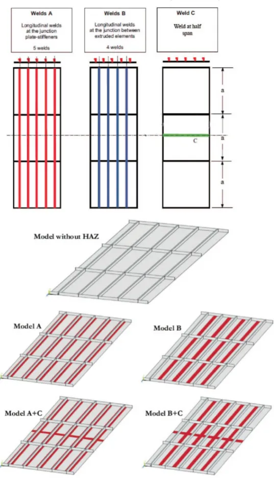
Five different finite element models are considered for analysis purposes (Figure 7). They are different in arrangement of HAZ zones; however, the geometrical imperfection is considered for all of them. They are the following:

• The reference model (WHAZ): the model without considering any HAZ.

• The model A: the model with five longitudinal welds along the junction lines between the plate and five stiffeners.

• The model B: the model with four longitudinal welds at the intersections between the plate and in which five extruded elements exist.

• The model A+C: the model in which, in addition to the welds as described in case of the model A, one line of transversal weld C also exists.

• The model B+C: the model in which, in addition to the welds as described in case of the model B, one line of transversal weld C also exists.

HAZ width equal to 2 × 25 mm in the plating and 25 mm in the stiffener web plates, all measured on the mid-planes of plate and stiffener, is shown in Figure 8. It is worth nothing here that the breadth of the elements of the finite element model is 25 mm. Thus, because this is the same breadth considered for the HAZ on each side of the weld line, the mechanical properties of HAZ material (see Figure 2) are attributed to the element in rows on both sides of each weld line.

The shortlisted parameters such as HAZ arrangements A, B, A+C and B+C (the combination of the HAZ arrangements that is illustrated in Figure 7) and model WHAZ are what has been proposed by Rigo et al. Furthermore, the initial shapes of spans CIP, CIS and Thin horse are the possibilities for the initial imperfection type based on Park's and Rigo's proposals and observations. All these factors are considered by the authors to cover all the possible cases of initial imperfection that arose from welding procedure. In this regard the authors had to abide by what the chief researchers of this field (Professors Paik and Rigo), had issued in their papers. 2.7. Tracing the average stress-average strain curve

Calculation of the ultimate strength or limit load of a structural model is a non-linear problem. Generally, the non-linear behaviour includes a wide variety of phenomena interacting with each other and in most cases they are difficult to calculate. In structural mechanics, the following two types of non-linearity may be accounted for: (1) Material non-linearity, which are functions of the state of stress or strain. Non-linear elasticity and yielding are the most notable examples.

(2) Geometric non-linearity, in which due to large deformations the equilibrium equations must be written with respect to the deformed structural geometry. Besides, the loads may change course as they increase.

Some equation-solving techniques are more applicable for the non-linear equations. Cook et al. (2002) and Paik and Thayamballi (2003) have introduced some of these methods. Among these techniques include Raphson method modified Raphson method and Arc-Length method. In this study, the Newton-Raphson method which is an iterative method for solving non-linear equations, is adopted. Both material and geometric non-linearities are considered in the analyses. Figure 9 illustrates the entire process of problem solving in this paper in a nutshell. This figure presents the important remarks of this study.

3. Results and discussion

In the analyses conducted in this study, one aluminium panel with predefined geometrical specification has been considered and the effects of different factors have been investigated based on complicated finite element modelling and analysis. The effects of different HAZ arrangements, different levels of lateral water height and various geometrical imperfection types have been investigated.

(10)

Figure 7. Analysis models with difference in HAZ arrangement. (This figure is available in colour online.)

The results of these analyses are presented in different sets of tables and figures, in order to facilitate the study and comparison of the results and to enable the reader to distinguish the influences of these factors on the

(11)

behaviour of the stiffened aluminium plate. In this regard Tables 2-6 demonstrate the results of the cases under combined longitudinal compression and different levels of lateral water heights of 0, 2.5, 5, 10 and 12.5 m, respectively. The results in these tables have been classified based on the imperfection types and HAZ arrangements. In every set of the results (thin horse, CIP and CIS modes), the results are compared with those corresponding to the case of reference model 'WHAZ'. Also, another comparison of the results in each case with those corresponding to the case of pure in-plane compression loading is given in another row in Tables 3-6. Furthermore, Tables 7-11 represent the stress ratio results of analysis cases under combined longitudinal compression and different levels of lateral water heights of 0, 2.5, 5, 10 and 12.5 m, respectively. The classification of the results in these tables is the same as that in Tables 2-6. They tend to express the post-yielding load-carrying capacity of the models and the influence of different factors affecting them. Moreover, for better comparison of the results, they are also presented graphically in Figures 10-14, based on the HAZ

arrangements of the models.

Figure 8. HAZ width in plates and stiffeners. (This figure is available in colour online.)

(12)

Table 2. Ultimate strength of models under pure compression (lateral water height = 0).

With HAZ

Contributors Load-carrying capacity Without HAZ

(Reference) Model A Model B Model A+C Model B+C Thin horse type imperfections models

Present study Max. average stress (MPa) Value 162.79 143.64 159.07 124.6 142.56

Difference to reference (%) Ref. -11.76 -2.28 -23.46 -12.42 CIP-FROTY type imperfections models

Difference to reference (%) Ref -11.41 -0.47 -11.71 -1.01 CIS-FROTY type imperfections models

Difference to reference (%) Ref -10.81 -0.23 -10.99 -0.4

Table 3. Ultimate strength of models in analysis case with 2.5 m lateral water height.

With HAZ

(Reference) Model A Model B Model A+C Model B+C Thin horse mode type imperfections models

Difference to reference (%) Ref. -12.25 -1.34 -23.33 -17.1

Difference to H = 0 (%) -1.36 -1.9 -0.42 -2.51 -6.6

CIP-FROTY type imperfections models

Difference to H = 0 (%) 3.89 3.91 3.82 4.17 3.14

CIS-FROTY type imperfections models

Difference to H = 0 (%) 9.51 8.1 9.4 9.9 9.26

Table 4. Ultimate strength of models in analysis case with 5 m lateral water height.

With HAZ

Difference to H = 0 (%) -6.42 -6.86 -5.55 -4.3 -6.94

Difference to H = 0 (%) 4.24 2.21 4.4 0.044 0.43

Difference to H = 0 (%) 11.38 8.16 11.08 4.12 5.04

Table 5. Ultimate strength of models in analysis case with 10 m lateral water height.

With HAZ

(13)

Difference to H = 0 (%) -10.64 -19.97 -23.81 -10.75 -15.45

Difference to H = 0 (%) -6.85 -8.73 -6.62 -13.51 -10.84

Difference to H = 0 (%) -5.78 -7.88 -8.51 -12.8 -11.93

Table 6. Ultimate strength of models in analysis case with 12.5 m lateral water height.

With HAZ

Difference to H = 0 (%) -30.99 -28.04 -34.4 -29.74 -29.2

Present study Max. average stress (MPa) Value 109.2373 85.45 105.337 85 100.86

Difference to H = 0 (%) -14.4 -24.38 -17.06 -24.51 -20.19

Difference to H = 0 (%) -14.24 -17.98 -20.77 -24.58 -21.13

Table 7. Comparison between (σiy/σY) and (σu/σY) for analysis case of pure compression.

With HAZ

Contributors Load-carrying capacity Without

HAZ Model A Model B Model A+C Model B+C Thin horse type imperfections models

Present study Initial yield stress/yield stress (σiy/σY) Value 0.55 0.49 0.49 0.49 0.48

Max. average stress/yield stress (σu/σY) Value 0.62 0.55 0.61 0.52 0.54

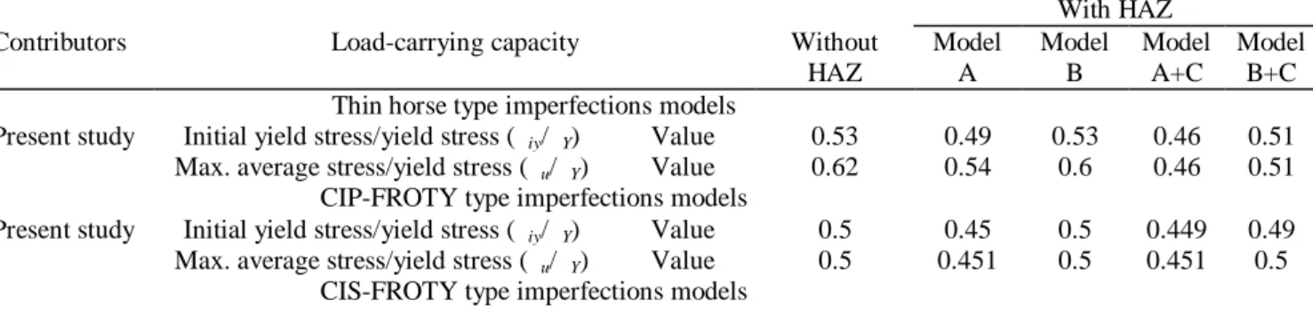
Table 8. Comparison between (σiy/σY) and (σu/σY) for analysis case of 2.5 m lateral water height.

With HAZ

Contributors Load-carrying capacity Without

HAZ Model A Model B Model A+C Model B+C Thin horse type imperfections models

(14)

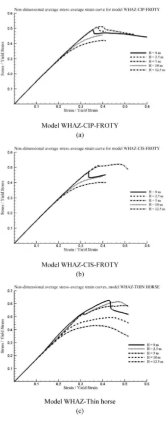
Figure 10. Non-dimensional average stress-average strain curve for model WHAZ: (a) Model

(15)

Figure 11. Non-dimensional average stress-average strain curve for model A: (a) Model A-CIP-FROTY; (b)

Model A-CIS-FROTY; (c) Model A-thin horse.

Table 9. Comparison between (σiy/σY) and (σu/σY) for analysis case of 5 m lateral water height.

With HAZ

Contributors Load-carrying capacity Without HAZ Model

A Model B Model A+C Model B+C Thin horse mode type imperfections models

(16)

Max. average stress/yield stress ((σu/σY) Value 0.58 0.51 0.57 0.46 0.51

Max. average stress/yield stress ((σu/σY) Value 0.51 0.44 0.51 0.433 0.48

Table 10. Comparison between (σiy/σY) and (σu/σY) for analysis case of 10 m lateral water height.

With HAZ

A Model B Model A+C Model B+C Thin horse type imperfections models

Present study Initial yield stress/yield stress (σiy/σY) Value 0.278 0.3 0.265 0.25 0.265

3.1. Verification of code and modelling approach

One of the most important requirements of any finite element analyses is verification of the code and modelling procedure. For this reason, the results of the present modelling and analyses are compared with the investigation results of Committee III.1 'Ultimate Strength' of ISSC'2003 on the same panel. As shown in Table 12, good agreements are observed between the analysis results of corresponding models. It should be mentioned here that the analyses are based on the boundary conditions used by the Committee in their investigations, i.e. the nodes on mid-transverse frames are restrained from moving in z direction (W = 0 at mid-frames). For lower lateral pressure as well as for pure compression, the above-mentioned point about boundary condition does not affect the panels' ultimate strength significantly (Tables 2 and 12).

Table 11. Comparison between (σiy/σY) and (σu/σY) for analysis case of 12.5 m lateral water height.

With HAZ

A Model B Model A+C Model B+C Thin horse type imperfections models

Table 12. Comparison between the results of analyses done by various researchers.

With HAZ

(Reference) Model A Model B Model A+C Model B+C

(17)

(2003) (MPa) Difference to reference (%) Ref. -13.40 -1.30 -25.56 -12.60 Lehmann (Rigo

et al. 2003)

Max. average stress (MPa)

Value 169.88 144.48 161.47 125.81 141.94

Difference to reference (%) Ref. -16.71 -6.91 -27.47 -18.17 Yao (Rigo et al.

2003)

Value 160.80 136.15 157.7 126.1 146.28

Khedmati et al. (2010)

Value 166.63 145.27 159.33 134.97 145.68

Difference to reference (%) Ref. -12.81 -4.38 -19.00 -12.57 Present study Max. average stress

(MPa)

Value 161.28 143.13 158.49 123.1 142.24

3.2. Analysis cases of pure in-plane compression

In this case, the models are tested in pure in-plane compression situation. According to Table 2, the model WHAZ-thin horse, with ultimate strength of 162.72 MPa, exhibits the maximum and the model A+C-CIS, with 108.37 MPa, exhibits the least ultimate strength. All models with thin horse mode of initial imperfections are of more strength compared to their CIP or CIS counterparts. Furthermore, the CIP models are of more strength compared to the CISs.

The reason for this is the initial shape of the models. The longitudinal stiffeners at the mid-span of CIS type models are likely to be in a compressive situation. When the analysis starts, they are more compressed. With this kind of initial imperfection, the compressive load is exerted on them with eccentricity. The initial yielding occurs in the stiffeners of this span, and because of further compression they collapse and the load-carrying capacity of the panel reduces.

In CIP models, stiffeners in two side spans are in compressive initial situation. During analysis, yielding begins from the stiffener in these two spans, but these models are stronger than their corresponding CIS type, and it clarifies the importance of the position of the span with compression in stiffeners.

In models with initial imperfections in thin horse mode, the plates of all spans are in compressive situation from the beginning of the analysis. Therefore, yielding begins soon after ultimate strength stage and at this stage yielding is observed in a wide range in plates and stiffeners. In CIS and CIPs, however, the plates are with sinusoidal distortions and the beginning of yielding is almost concurrent with ultimate strength stage. Insignificant difference between ultimate strength of model B and WHAZ in CIS and CIPs is noticeable. It denotes the importance of the imperfection mode compared to HAZ arrangements. Furthermore, existence of a transverse weld line in the models B+C and A+C, both in CIS condition, has the least effect on their ultimate strengths. It ascertains the need for a good knowledge of the initial imperfection modes for conducting finite element analysis with a great level of accuracy and reliable results, from the design optimisation point of view. Figure 15 illustrates model B with different initial imperfections mode in pure compression situation. According to Figure 15a, in models with thin horse mode

imperfections, yielding begins in a wide range in plates and stiffeners. As the analysis continues, at final stages of analysis, accumulation of plasticity is observed in mid-length of models in both plates and stiffeners. In A+C and B+C, this is followed by folding mode of deflection in the middle span of the model around the transversal weld line (Khedmati et al. 2009). However, for CIP and CISs, accumulation of plasticity in stiffeners is enough for the panel to collapse. In other words, the yielding initiates at the most critical points that are indicated in red in Figures 15b and 15c. It is observed from Figure 15b that the most critical point of the models with CIP type initial imperfections are the flanges of the stiffeners at the middle length of two side spans. After initiation of yielding at these critical points, due to further action of the compressive load in later stages of the analysis, the stiffeners collapse by severe plasticity accumulation and flexural and torsional deformations. The same collapse pattern is observed in the models with CIS-type initial imperfection. However, the positioning of the critical points is different. In these model sets (CIP and CIS), existence of a transverse welding line does not affect the strength of the panel very much as it is understood from Table 2.

(18)

Figure 12. Non-dimensional average stress-average strain curve for model B: (a) Model B-CIP-FROTY; (b)

(19)

Figure 13. Non-dimensional average stress-average strain curve for model A+C: (a) Model A+C-CIP-FROTY;

(20)

Figure 14. Non-dimensional average stress-average strain curve for model B+C: (a) Model B+C-CIP-FROTY;

(21)

Figure 15. Deflection mode and spread of yielding at stage of yielding initiation: (a) Model B-thin horse; (b)

(22)

The stress ratios of the models under pure compression are given in Table 7. For thin horse mode models, significant difference is observed between stress ratios. It implies that after initiation of yielding until ultimate strength stage, the panel still has load-carrying capacity. Beam-column-type initial deflections of the stiffeners, in addition to the sinusoidal deformations of the plating, lead to beginning of yielding and attaining ultimate strength at the same stages of analysis as in the case of the CIP and CIS models.

3.3. Analysis cases of 2.5 m lateral water height

The results for the case of combined uniaxial in-plane compression and 2.5 m lateral pressure in Table 3 reveal that compared to the case of pure compression loading, some reduction in the yield strength is observed for thin horse models. The maximum and minimum amounts of reduction in the yield strength are about 6.6% for the model B+C-thin horse and about 0.42% for model B-thin horse, respectively (see c indexed parts of Figures 10-14). The ultimate strength of all CIS and CIP models show some increase in value. Because of this amount of lateral pressure, CIS models are of more strength compared to the CIP ones (see parts a and b of Figures 10-14). This is mainly due to delay in collapse of stiffeners and propagation of yielding. In fact, the 2.5 m water height lateral pressure acts as an obstacle against the beam-column-type deflections of stiffeners within their mid-spans. In thin horse models, however, this amount of lateral pressure weakens the panels and makes yielding to happen sooner. In CIS models, the maximum increase of ultimate strength is observed compared to the pure

compression condition. From Table 3 it is clear that the highest and lowest bonds of the strength increase are corresponding to the models A+C-CIS with 9.9% and B+C-CIP with 3.14%, respectively.

Similar to the case of pure compression, a transverse weld line does not affect the strength of CIS and CIP models as it significantly affects the thin horse models. For example, compared to the reference model WHAZ, the strength of model A+C-thin horse is less than that of model A-thin horse. While in the CIP and CIS model sets, as the results of the A+C-CIP and CIS are compared to their corresponding A models, the strength reduction is less significant (see Table 3).

Data in Table 8 show that in thin horse set models, yielding does not occur at ultimate strength stage, except for models A+C and B+C. Compared to models A and B, a transverse weld line significantly affects their strength. As discussed earlier, the most sensitive span is the middle one, in which, at final stage of analysis, folding around transverse line is observed, and it is the rationale for the concurrency of the yielding occurrence and the collapse of the panel.

In CIS models, yielding begins from junction of longitudinal stiffeners with frames of both ends. So, until ultimate strength stage in which stiffeners of mid-spans collapse by severe yielding and tripping, panels still have load-carrying capacity; however, in CIPs the yielding pattern is different. This is more clarified by the data presented in Table 8, which proves significant difference between (σu/σY) and (σiy/σY) for CIS models in

comparison to those for CIP models. In the models of CIP set, yielding begins at the two side spans of the longitudinal stiffeners that are subject to compression from the earliest stage of the analysis, and this amount of lateral pressure induces more compression in these stiffeners. Therefore, yielding in the two side spans of the longitudinal stiffeners associated with their tripping mode deformation results in a sudden drop in the load-carrying capacity after yielding collapse of the panels, irrelevant of their HAZ arrangements.

3.4. Analysis cases with 5 m lateral water height

The results for the case of combined uniaxial in-plane compression and 5 m lateral pressure are presented in Table 4. Compared to the case of pure in-plane compression, the ultimate strength in thin horse set models decreases. The maximum reduction in the ultimate strength is about 6.94%o for the model B+C-thin horse (see part c of Figures 10-14). In this set of the models, the least strength is for A+C-thin horse, which shows 21.71% strength reduction compared to their corresponding reference models (WHAZ-thin horse models). Due to this amount of lateral pressure and this type of geometrical imperfection, the HAZ arrangement has a significant effect on the strength of the models. For example, addition of a transverse weld line to the model A-thin horse having an ultimate strength of 133.78 MPa leads to the model A+C-thin horse with the ultimate strength of 119.234 MPa.

Some non-uniform increase in the strength is observed for the CIP set models. The course of strength increases in A+C-CIP and B+C-CIP models, 0.044% and 0.43% respectively, and varies a significantly with the other models of this set. Furthermore, model B is seen to be almost as strong as reference model WHAZ. In the models of this set, a transverse weld line does not affect the strength of models noticeably. Similarly, strength of all models in CIS set increases; however, it is less significant for some of them. This can be well understood by

(23)

comparing the results presented in the last row of Table 4. Also, the strength of CIS models is more than their corresponding CIP models, which indicates that the same collapse pattern governs the behaviour of the models in this range of lateral water height.

The increase in lateral water pressure, as shown in Figures 16a-16c, makes the location of critical zones to change. They shift towards the junction of transverse frames and longitudinal stiffeners. According to Figure 16a, this shift is more significantly observed in the models with thin horse mode imperfections; therefore, they are more fragile compared to their CIP and CIS counterparts.

Figure 16. Deflection mode and spread of yielding at ultimate strength stage, analysis case with 5 m lateral

water head: (a) Model B-thin horse; (b) Model B-CIP-FROTY; (c) Model B-CIS-FROTY. (This figure is available in colour online.)

(24)

According to Figure 16b, the place of the tripping of the stiffeners and plasticity accumulation at the ultimate strength stage shifts towards the junction of the stiffeners with mid-frames (T2 and T3). According to Figure 16c, tripping of stiffeners, which was more likely to happen at mid-length of the mid-span in pure compression load condition, now happens near the T3 and T4 frames and all of these discrepancies are the result of the initial shape of the panels' spans. Despite all the above-mentioned discrepancies, a common point is noticeable in all sets; model B exhibits the least difference in strength with reference WHAZ models.

According to the results presented in Table 9, in thin horse model set, yielding begins before ultimate strength stage and after initiation of yielding, load-carrying capacity is still noticeable in all models of this set, except for A+C-thin horse. This amount of lateral pressure makes yielding to happen at an earlier stage compared to ultimate strength stage in CIP set except for B+C model. In CIS set, as the former case, the difference between (σiy/σY) and (σu/σY) is more than the models in CIP set, and this is due to the same yielding pattern, which was

explained in Section 3.2.

3.5. Analysis cases with 10 m lateral water height

With this amount of lateral pressure, apparently larger deflections are expected in models. Furthermore, tripping and yielding of stiffeners occur near their junction with transverse frames, especially the more solid ones (T1 and T4). Plasticity accumulation at these points and large deformation due to this amount of lateral pressure reduces the ultimate strength of all models significantly This amount of lateral pressure makes yielding to happen in an earlier stage in thin horse set. Due to this pressure, yielding occurs in lower axial average strain. With further increase of axial strain, models reach their ultimate strength by wide range yielding of stiffeners.

According to Table 5, in this case and due to this amount of lateral pressure, the ultimate strength of all models reduces, compared to the results of H = 0 case. Surprisingly, the maximum reduction is related to the model B-thin horse, which is one of the strongest models in this loading condition. In this regard, the strength reduction is much more noticeable in the thin horse models set. At the earliest stage of the analysis, the plates at the three spans were in the compression states. Due to this lateral water height and by further inward movement of the panel's edge, the longitudinal stiffeners and their adjacent plating (especially in the HAZs) near both ends start to yield and endure large deformation.

As shown in Table 5, unlike two former cases, in this situation, the strength of the CIP models is more than their corresponding models in the CIS model set. Under this loading condition, the critical points are around the junction of the longitudinal stiffeners and transverse frames, especially the more solid ones. The CIS models have two spans with the plating in the compression. Due to the direction of axial and lateral loading, the deformations and yielding would occur in earlier stage of analysis in the critical areas of the panels. This will result in strength reduction of the CIS models compared to CIPs. Further investigation into the results explains the importance of the HAZ arrangement. In all three sets, the model A+C exhibits the least strength. Moreover, A+C-CIS presents the most fragile structural combination with an ultimate strength of 94.51 MPa.

In both CIP and CIS model sets, difference between (σiy/σY) and (σu/σY) increases, which proclaims that yielding

initiates in stiffeners due to lesser axial strain (Table 10).

From the results in Table 10, it is understood that in all model sets, WHAZ model has the most post-yielding load-carrying capacity. In this regard, model B is in second rank in all sets. Therefore, the more the ultimate strength of the model, the later it collapses when yielding occurs. A comparison of the result of model B with B+C clarifies how a transverse weld line diminishes this advantage.

Despite the fact that in this loading condition the strength of CIP models is more than their corresponding CIS models, the post-yielding load-carrying capacity of the CIP models does not follow the same principle, indicating that as the yielding begins at the most critical points of the panels (as they were referred to earlier in this section), the initial conditions of the spans are the most important factors in addressing this issue under various load conditions. In this regard, the initial yield stresses of the models in the thin horse model set are less compared to those of their corresponding models in the CIP and CIS model sets.

3.6. Analysis cases with 12.5 m lateral water height

According to Table 6, compared to the case of pure compression (H = 0), in thin horse model set, maximum reduction of strength pertains to model WHAZ, and it is about 30.99%. Nevertheless, it reads from the table that the WHAZ-CIP and CIS models have the least strength reduction, which is about 14.4% and 14.24%o

(25)

respectively (see and compare the results in Figure 10).

The models in this analysis tend to follow the same yielding and collapse pattern as shown in the previous analysis. Therefore, the CIP models are stronger than their corresponding CIS models. Model B-CIS (89.057 MPa ultimate strength and 17.98% strength reduction), however, is an exception as it shows more strength and less strength reduction compared to model B-CIP (85.45 MPa ultimate strength and 24.38% strength reduction).

Figure 17. Deflection mode and spread of yielding at ultimate strength stage, analysis case with 12.5 m lateral

water head: (a) Model B-thin horse; (b) Model B-CIP-FROTY; (c) Model B-CIS-FROTY. (This figure is available in colour online.)

(26)

Figure 18. Ultimate compressive strength for all models under different levels of lateral pressure: (a) CIP

imperfection type models; (b) CIS imperfection type models; (c) Thin horse imperfection type models.

(27)

According to Figures 17a-17c, under this loading situation, the models with all three geometrical imperfections will reach their ultimate strength stage very early. It is associated with stiffener tripping near the T1 and T4 transverse frame and severe yielding at mid-transverse frames and membrane type over all deformation of the panel. Ultimate strength of corresponding models in sets does not vary much (see Table 6). This clarifies that in this case the strength of models depends on assembling sequence rather than initial imperfection type.

In this situation, as shown in Table 11, the post-yielding strength of the panels is much lesser compared to the former load combination cases. According to Table 11, as in case of 10 m lateral pressure, yielding strength of thin horse set models are less than the two other sets. This is because of the initial shape of models' spans, which is explained in the previous section. For example, the A+C-thin horse model has the least yielding strength (σiy/σY = 0.187); however, it has more post-yielding load-carrying capacity compared to its CIP and CIS

counterparts. Furthermore, all corresponding models within different models set have almost an equal (σu/σY)

ratio. It is due to the similarity in collapse pattern of the models in this loading situation. 3.7. Summary

In thin horse models (Figure 18a), due to all amounts of lateral pressure, model WHAZ and A+C exhibit the maximum and minimum values of ultimate strength, respectively. In these models, existence of a transversal weld line has a significant effect on strength of panels. With the increase in lateral pressure, strength reduction in all models is observed. Model B performs the best behaviour between all welded models compared to reference WHAZ model. It should be noticed that with further increase in lateral pressure, the difference between the strength of these two models grows as it is obvious in 10 m and 12.5 m water height in Figure 18a.

In CIP- and CIS-type imperfection models, like thin horse models, for the entire range of lateral pressures, WHAZ and A+C models exhibit the maximum and minimum values of ultimate strength, respectively. The difference between the strength results of A, A+C and B, B+C models is less than their thin horse counterparts. This emphasises that the imperfection type is of primary importance. Not including the exceptional cases, with a 2.5 m and 5 m lateral pressure, strength of all models in these two sets increases compared to the case of pure compression. It should be noted that the CIS models' strength increases or decreases at a higher rate.

The effect of the transversal weld line on the ultimate strength is less than CIP-type models. This is implicit from Figures 18b and 18c. Because of a higher lateral water height, this effect is more significant. Unlike the other three models (WHAZ, A and B) in their corresponding model set, models A+C and B+C, in both CIP and CIS model sets, show an increase in strength only due to increase in the water height from 0 m to 2.5 m.

4. Conclusions

• In models with thin horse mode imperfections, independent of the HAZ arrangement, increase in lateral pressure leads to decrease in strength. However, in models with CIP and CIS imperfection types, by increasing the pressure, the strength first rises (stress has a beneficial effect) and then falls (pressure is detrimental). This is due to the different curvatures of spans in these models, which are dominantly affected by column-type

deflection of stiffeners. A small lateral pressure delays the collapse of these stiffeners.

• In the three different model sets, HAZ arrangement does not affect the general form of the average stress-average strain curve (see Figures 10-14).

• Tripping and yielding of stiffeners are the major collapse modes observed in all models in ultimate strength and final stage of analysis. These collapse modes are independent of the deflection imperfection type. Deflection imperfections only affect the location of tripping occurrence. It occurs at mid-length of spans due to lateral water height of 0 m, 2.5 m and 5 m and at intersections of longitudinal stiffeners and transverse frames due to 10 m and 12.5 m lateral water height.

• Generally, for all the range of lateral pressure, model A+C in CIP or CIS model set has the least strength. When the water height is 2.5 m and 5 m, A+C-CIP behaves the worst. This is true for model A+C-CIS when lateral pressure is 0 m, 10 m and 12.5 m.

• For the low amount of lateral pressures, B-CIP or B-CIS models have the ultimate strength almost equal to their corresponding without HAZ reference model. But for higher level of lateral pressure, the B model has significantly smaller strength compared to WHAZ model.

(28)

• Concerning initial deflection imperfections, for lateral pressure of 2.5 m and 5 m, strength of CIS models is more than the strength of CIP ones. The lateral pressure acts as a barrier against large deformation of sensitive mid-span in CIS models. For CIP models, the sensitive spans are the side ones, and compared to the CIS models these amounts of lateral pressure collapse the stiffener in the sensitive spans at earlier stages. Therefore, the ultimate strength in CIP models is less than that in CIS models.

• Among models with thin horse imperfections, it is rare that the ultimate strength occurs at final stage of analysis (without post-collapse curve). There is always load-carrying capacity after ultimate strength stage. For CIP and CISs, however, due to existence of local plate buckling type deformations between stiffeners, the post-ultimate strength load carrying is reduced, or in some cases it is almost zero (see (a) and (b) indexed part of Figures 10-14).

• In the case of lower lateral pressure and pure compression, there is large difference between the results of corresponding models in sets. For higher lateral pressure, the difference of the result of corresponding models in three sets becomes lower. In fact, the HAZ arrangement (compared to deflection imperfection type) dominates strength of the models for high lateral pressure.

• For all analysis and geometrical imperfection types, the B models have the best behaviour within the considered welding schemes and it is highly recommended that this assemblage sequence is used in fabrication of aluminium panels.

• Because there are several points taken into consideration in this study, and they are all interacting with one another during the analysis with all their nonlinear effects, the behaviour of a certain model could not be concluded based on the results already obtained in the other analysis. In this regard, all models with their relevant conditions should be investigated specifically and then reasonable conclusion must be made for design purposes. However, there are still some observations that are common for all models included in a specific analysis. In this regard, one of the most noticeable points is that the model A+C is the weakest model compared to the model WHAZ in all model sets, and therefore it is highly recommended that the designers avoid such structural combination (HAZ arrangement) in planning their panels especially where the structure is intended to endure severe sea states.

According to the results of the present study, it is confirmed that assessment of ultimate strength of the panels by non-linear finite element analysis is highly dependent on the imperfections type, especially the geometrical ones. Generally, there are several welding methods that could be used for building aluminium structures such as FSW, GMAW, etc. These welding methods have specific effects on imperfections that have to be carefully studied through wide ranges of experimental studies, such as investigations of Paik et al. (2008) and Park (2009). The results of the present study explain the need for a subtle identification of the welding-induced imperfections, especially in structures like catamarans and ferries that are designed to operate in severe sea conditions. References

Aalberg A, Langseth M, Larsen P. 2001. Stiffened aluminium panels subjected to axial compression. Thin-Walled Struct. 39(10):861-885.

ANSYS. 2007. ANSYS user's manual release 11.0. Canonsburg (PA): ANSYS.

Benson S, Downes J, Dow R. 2011. Ultimate strength characteristics of aluminium plates for high-speed vessels. Ship Offshore Struct. 6(1-2):67-80.

Clarke J, Narayanan R. 1987. Buckling of aluminium alloy stiffened plate ship structure. Paper presented at the proceedings of the International Conference on Steel and Aluminium Structures; Cardiff, UK.

Collette M. 2005. Strength and reliability of aluminium stiffened panels [doctoral thesis]. [Newcastle upon Tyne (UK)]: School of Marine Science and Technology, Faculty of Science, Agriculture and Engineering, University of Newcastle.

Cook R, Malkus D, Plesha M, Witt R. 2002. Concepts and applications of finite element analysis. New York: Wiley.

Herrington P, Latorre R. 1998. Development of an aluminium hull panel for high-speed craft. Mar Struct. 11(1-2):47-71.

Hopperstad O, Langseth M, Hanssen L. 1997. Ultimate compressive strength of plate elements in aluminium: correlation of finite element analyses and tests. Thin-Walled Struct. 29(1-4):31-46.

Khedmati MR, Bayatfar A, Rigo P. 2010. Post-buckling behaviour and strength of multi-stiffened aluminium panels under combined axial compression and lateral pressure. Mar Struct. 23(l):39-66.

(29)

Khedmati MR, Ghavami K. 2009. A numerical assessment of the buckling/ultimate strength characteristics of stiffened aluminium plates with fixed/floating transverse frames. Thin-Walled Struct. 47(11):1373-1386.

Khedmati MR, Zareei MR, Rigo P. 2009. Sensitivity analysis on the elastic buckling and ultimate strength of continuous stiffened aluminium plates under combined in-plane compression and lateral pressure. Thin-Walled Struct. 47(11): 1232-1245.

Kim UN, Choe IH, Paik JK. 2009. Buckling and ultimate strength of perforated plate panels subject to axial compression: experimental and numerical investigations with design formulations. Ship Offshore Struct. 4(4):337-361.

Kristensen Q, Moan T. 1999. Ultimate strength of aluminium plates under biaxial loading. Paper presented at the proceedings of the International Conference on Fast Sea Transportation; New York, USA.

Paik JK. 2009. Buckling collapse testing of friction stir welded aluminium stiffened plate structures. Report SR-1454. Washington (DC): Ship Structure Committee.

Paik JK, Thayamballi AK. 2003. Ultimate limit state design of steel plated structures. 1st ed. London: John Wiley & Sons.

Paik JK, Thayamballi AK. 2006. Some recent developments on ultimate limit state design technology for ships and offshore structures. Ship Offshore Struct. 1(2):99-116.

Paik JK, Thayamballi AK, Ryu J, Jang J, Seo J, Park S, Soe S, Renaud C, Kim N. 2008. Mechanical collapse testing on aluminium stiffened panels for marine applications. Report SSC-451.1232-1245. Washington (DC): Ship Structure Committee.

Rigo P, Sarghiuta R, Estefen S, Lehmann E, Otelea S, Pasqualino I, Simonsen BC, Wan Z, Yao T. 2003. Sensitivity analysis on ultimate strength of aluminium stiffened panels. Mar Struct. 16(6):437-468.

Sielski RA. 2008. Research needs in aluminium structure. Ship Offshore Struct. 3(1):57-65.

Zha Y 2003. Experimental and numerical prediction of collapse of flatbar stiffeners in aluminium panels. J Struct Eng. 129:160.

Zha Y, Moan T. 2001. Ultimate strength of stiffened aluminium panels with predominantly torsional failure modes. Thin-Walled Struct. 39(8):631-648.