HAL Id: hal-02287247
https://hal.archives-ouvertes.fr/hal-02287247
Preprint submitted on 13 Sep 2019HAL is a multi-disciplinary open access archive for the deposit and dissemination of sci-entific research documents, whether they are pub-lished or not. The documents may come from teaching and research institutions in France or abroad, or from public or private research centers.
L’archive ouverte pluridisciplinaire HAL, est destinée au dépôt et à la diffusion de documents scientifiques de niveau recherche, publiés ou non, émanant des établissements d’enseignement et de recherche français ou étrangers, des laboratoires publics ou privés.
Repetitive control for magnetic flux control
Pierre Haessig
To cite this version:
Repetitive control
for magnetic flux control
Pierre Haessig (IETR, CenraleSupélec, Rennes) June – September 2019
1
Introduction
1.a Context
This draft memo describe my learning and some experiments with the so-called repetitive control, for the purpose of controlling the magnetic flux in a test bench for loss measurement in magnetic materials. This exploration is a follow-up on a June 2019 discussion with Anh-Tuan Vo and Afef Lebouc from G2Elab/MADEA, two co-authors of the article « Nouvelle commande adaptive pour des mesures magnétiques sous conditions d’excitation complexes »[1] presented at JCGE 2019 in Oléron. This repetitive control, which I had read about some years ago, may be useful in this context, because it promises to track
a periodic reference signal with zero steady state error and very few parameters to tune. This
is precisely the requirement for the magnetic test bench.
1.b About the magnetic measurement test bench
The test bench is described in Vo’s article [1], from which I reproduce the functional diagram in Figure 1.
Figure 1: Functional diagram of the closed-loop control of the magnetic test bench of Vo and
colleagues[1]. The objective is to control the magnetic flux inside a test material placed in an “Epstein frame” by injecting an excitation current I1. The magnetic flux is not directly measurable, but the
measured voltage V2 is proportional to its derivative. Comparing this feedback measurement with a flux
reference signal (not depicted), the Labview controller generates a voltage Vsortie for the power amplifier
AE TECHRON which ouputs a proportional voltage V1. This voltage in turns generates the excitation
This closed-loop control system can be run with many control algorithms (cf. Vo), with some key features of the control problem being:
1. There exist a physical model of the controlled system based on transformer equations.
2. Yet, the model is not precisely known. Indeed, there are non-linearities and uncertain parameters in the Epstein frame (e.g. leaks) and material itself (since the goal of the setup is to characterize it!).
3. A very low tracking error should be achieved. 4. The reference signal known in advance and periodic
First, the existence of a model of the system (typically V2 is approximately proportional to V1, with a known ratio) implies that some feedforward (open-loop) control can be used. This practically means precomputing a trajectory for Vsortie based on the flux reference trajectory. This is a good starting point.
However, features 2 and 3 imply that open-loop control does not perform well enough, and neither does a simple closed loop control algorithm (like PI). More advanced control is needed. The final feature means that some kind of learning-based control can be used to exploit the knowledge of the reference signal. Vo’s article provides such a scheme. In this document, we explore an alternative named “repetitive control”.
2
Repetitive control
2.a Introduction to repetitive control
Repetitive control comes from Japan in the 1980s. It is advertised as a simple learning scheme that can track a periodic reference signal with zero steady state error. We will discuss this claim. Interestingly, one of its earliest applications was magnetic (synchrotron magnet power supply [2]). A more general treatment of stability issues was reported in 1988 [3]. The control architecture used in this note is presented Figure 2 along with our notations. In addition to the caption, we can mention that the reference signal y* is meant to be periodic, with frequency f₀. We remind that e-ds is the Laplace transfer of delay of time d (s being the Laplace variable). The feedforward path, important for the good performance, has no influence on the closed-loop stability theory. Its tuning is based on the knowledge of the plant model: assuming the plant transfer H(s) can be approximated by its steady state gain H₀ (in the magnetic bench, it is the number of turns ratio), then, we can choose:
F=1/H₀ (1)
Compared to the historical article [3], the present regulator is the “modified repetitive controller” of their Fig 5, with a(s) = 1, system transfer G(s) = K.H(s) and low-pass filter q(s) = 1/(1+τcs), plus the feedforward path which was not relevant for the stability issues covered in their article.
Feedforward path excluded, this controller has three parameters: 1. Proportional feedback gain K
2. Repetition delay d
3. Low filter time constant τC, that we can also express as a cutoff frequency fC = 1/(2π.τC).
Simplicity guided us towards choosing a simple proportional gain K in the feedback path. In a sense, we are discussing here a “proportional repetitive control”. More complex transfer functions could be used, but we haven’t found a reason to do so yet.
Repetition delay should be set according to:
d = 1 f 0
−τC (2)
where 1/f₀ is the period of the periodic reference signal. In practice, the low-pass time constant should be smaller than this period, so that we can reason as if1 d ≈ 1/f₀. With this approximation in mind, we can give a qualitative explanation of the repetitive regulator block: the output is the sum of the present input plus a copy of its output memorized from a time d in the past. This explains the “repetitive” adjective. Keeping in mind that the tracking objective is to drive the signal ε to zero, we can understand that the repetitive regulator is feeding back to the plant a copy of the accumulated error from previous periods. If a zero steady state error is eventually reached, the repetitive block receives zero as input but can keep “replaying” the periodic signal it has learned to be appropriate to reach this steady state. This is why it can be seen as a simple learning-based control.
An alternative view on this controller comes from the Internal Model Control (IMC) principle. The repetitive control block in that view is a transposition of the integrator 1/s in the classical PI control from the case of constant reference signal to the case of periodic
1 Still, numerical experiments taught us that the correction by −τC, which compensates the phase lag of the
low-pass filter, is necessary for good tracking performance.
Figure 2: Controller architecture based on the repetitive control principle. System under control is the blue Plant, which includes a perturbation input w to account for plant modeling uncertainties.
Controller is the light yellow box, taking as inputs the reference signal y* and the plant measurement y. Controller output u is the sum of two paths: the feedforward path and the feedback path. Feedforward is important for the good practical performance of the control but is not related to the repetitive aspect of the controller. Our choice of feedback is a proportional gain K in series with the repetive regulator block in orange. The transfer of the entire feedback path u(s)/ε(s) is named C(s).
signals. Indeed, in the IMC view, the PI can track a constant reference because it has a pole at 0 Hz (s=0), so that in can generate a constant signal when its input is zero. Similarly, the repetitive control block has poles at s=j2π/d (≈j2πf₀) and all its harmonics, so that in can sustain a periodic signal of frequency f₀ when its input is zero.
Once the repetition delay d is set, there are two parameters left for the control tuning: gain K and time constant τC (or cutoff frequency fC).
2.b Tuning the repetitive controller
Tuning the two parameters of the proportional repetitive controller should be done with regards to three properties:
1. Stability: the closed-loop system should remain stable
2. Precision: the control error (difference between reference and measurement) in the periodic steady state should be small
3. Convergence speed: the periodic steady state should be reached reasonably fast After discussing these three criteria, we will formulate our recommendations for tuning at the end of this section.
Notice that for the last two criteria, quantitative targets may be set with a better knowledge of the application.
Stability
Stability is covered in the milestone 1988 article of Hara et al. [3]. To summarize, the open-loop complex gain of the system without the repetitive block, which is G(jω) with their notation and K.H(jω) here, should never enter a disc centered at z=-1 with radius being the gain of the low-pass filter placed in series with the delay. Below the cutoff frequency fC, this radius is 1, above it tends to zero so that the forbidden disc becomes the point z=-1. This shows that this low-pass filter is inserted to preserve the closed-loop stability. Also, since gain K scales the open-loop gain, there is a risk that too high a value destabilizes the system. For an illustration, see. The Nyquist plot on Fig 7 of [3], case a=1.
Conclusion: to keep the system stable, the gain K and the cutoff frequency fC should be chosen “small enough”.
Steady state precision
Remark: this criterion (low control error) is important of the scientific validity of the magnetic measurements to be realized with the test bench.
We analyze this property by computing analytically the rejection of the perturbation w (cf. Figure 2). Since we study a periodic regime a frequency f₀, we consider an harmonic perturbation at frequency n.f₀, with n=1,3,… (n is likely odd in the application).
Hypotheses of the following analysis:
• Plant gain H(j.n.f₀) is close to 1, meaning that:
◦ the perturbation is within the bandwidth of the plan
◦ for the test bench case, the number of turns ratio is one (if not, the formula below should be adapted, but the idea would be the same)
• the perturbation is within the bandwidth of the low-pass filter: n.f₀ < fC, but not necessarily much smaller
Then, our own calculations show that the transfer from perturbation to output (y(s)/w(s)) is approximately:
(
w (s )y (s))
s= j 2πf0 =1 K ( nf 0 fC ) 2 (3) Therefore, we see that the steady state error is not zero, as initially advertised in the presentation of the repetitive control. This is due to the addition of the low-pass filter, which is, as explained before, necessary for stability (removing the filter with fC → ∞indeed yields zero error). Now, analyzing formula (3), we see that:• low frequency harmonics are better rejected, with a quadratic effect of the harmonic rank n
• perturbation rejection can be improved by ◦ increasing feedback gain K
◦ increasing the cutoff frequency fC
These conclusions confront the previous conclusion on stability (K and fC should be “small enough”). This is a classical stability-precision tradeoff. However, our numerical experiments show that good precision can be reached easily.
Convergence speed
Another simplified calculation, neglecting the effect of the low-pass filter, shows that at each period, the residual error is multiplied be a factor small that one:
ε(t +T0)= 1
1+K . H ε(t ) (4)
This shows that the error decays geometrically, with the convergence speed dictated by the open-loop gain K.H. Notice that equation (4) implies that the error converges to zero, in contradiction with (3), but this is because we have neglected the low-pass filter in this section.
Tuning recommendations
These are recommendations with the magnetic test bench in mind, meaning that the plant transfer is assumed to some sort of low-pass filter, with a flat well-known gain in the plant bandwidth and with an approximately known cutoff frequency. Gain relates to the number of turns ratio. Bandwidth may be the bandwidth of the power amplifier.
I believe the loop gain KH should be set equal to a few units:
KH0=1 to3 (5)
This will enable a convergence after a few periods (perturbation error divided by 2 to 4 at each period).
Cutoff frequency should be chosen slightly smaller than the natural bandwidth of the system.
3
Numerical experiments
We run numerical experiments to validate our formulas from section 2.b. Numerical implementation was done in OpenModelica[4], an open-source Modelica-based modeling and simulation environment (available at https://openmodelica.org/). All the code is available at https://github.com/pierre-haessig/repetitive-ctrl-magnetic in the
MagneticTestCtrl.mo Modelica file (single package file).
Notice that, as a difference with Vo’s article [1], we choose to control not the B field but rather the actual output of the plant: voltage V2,which is the derivative of B (cf. Figure 1).
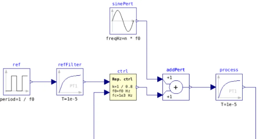
3.a Perturbation rejection and convergence speed
The first test is with a first-order model for the plant H(s) (following notation of Figure 2) presented. Schematic is on Figure 3. The static gain of the plant H₀ is set to 0.8, but for the purpose of tuning the feedforward path we pretend it is 1 (so F=1 according to (1)) so that the feedback path has some work left. This imitates an unknown 20% magnetic leakage in the real application.
Plant bandwidth is about 16 kHz (i.e. a first order time constant set to 10 µs). Therefore, fC, the cutoff frequency of the low-pass filter within the repetitive controller, is set to 1 kHz, which yields a stable closed-loop operation.
The periodic reference to be tracked is a 50 Hz square wave which imitates a triangular B field reference of the real application. A low pass filter smoothes this reference signal with the same cutoff as the plant. Finally, there is a harmonic perturbation at frequency n.f₀ like in the paragraph on perturbation rejection in section 2.b.
Figure 3: Repetive control of a first-order plant, with square reference signal and harmonic perturbation.
Perturbation rejection experiment
Purpose here is to validates the perturbation formula (3). We run three experiments with varying values of the proportional gain K (K=1 or 2) and rank n of the perturbation (harmonic 3 or 5). Perturbation amplitude is set to 1 to make it easy to visualize the y/w gain. We see that higher frequency perturbations are less rejected (quadratic effect). Increased gain K improves the rejection (linear effect). Increasing the cutoff frequency fC would also improve the rejection (quadratic effect), but increasing it too much would make the system unstable. Figure key: plant output in solid blue, reference is dotted blue,
perturbation in thin solid red.
150 Hz perturbation (n=3), K=1. Theoretical gain y/w = 0,011
150 Hz perturbation (n=3), K=2. Theoretical gain y/w = 0,0056
Convergence speed experiment
Purpose here is to validate the convergence speed formula (4). In these three experiments, the harmonic perturbation is set to zero to focus on the tracking transient. To make this transient more visible, we disable the feedforward path for the first two experiments. With a loop gain K.H equal to one, we can indeed see that the tracking error gets halved at each period. When K.H = 3, it gets divided by 4. Adding a feedforward F=1, even if 20% too small (it should be 1/0.8) strongly improves the transient.
Loop gain K.H=1, no feedforward (F=0)
Loop gain K.H=3, no feedforward (F=0)
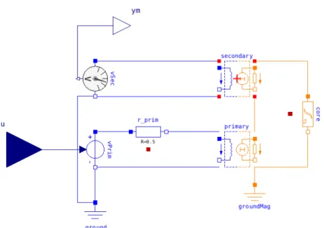
3.b Magnetic test bench
To make the simulation closer to the real application, we make a second test, visible on Figure 4, replacing the plant and the harmonic perturbation with a physical model which closely mimics the actual test bench. In particular, the non-linear material behavior (“soft magnetic hysteresis based on the Tellinen model and simple tanh()-functions” from the documentation)creates a perturbation-like effect due to the current spikes. Parameters of the material (which are default values of this model):
• Saturation polarization Js=1.8 T • Remanence Br=0.9 T
• Coercivity: 120 A/m
Reference voltage is a 50 Hz square wave of amplitude such that the B field in the material under test gets close to the saturation. The cutoff frequency of the low-pass filter fC is set to 1 kHz.
Figure 5: Physical model of the magnetic test bench. Plant input is a voltage source which feeds the primary side of a Epstein frame. Plant output is the voltage on the secondary. The magnetic material under test, named "core" has a non-linear B-H relation. It is the
GenericHystTellinenSoft model from Modelica Standard Library’s
Magnetic.FluxTubes[5] package.
Figure 4: Repetive control of a physical model of the magnetic test bench
Three experiments are run, first with K=1, without feedforward to better see the transient. With the feedforward and K=1, the transient becomes barely visible. Finally, without feedforward but gain increased to K=3, the fast convergence speed is observed.
K=1, no feedforward
K=1, with feedforward
4
Conclusions
It seems that repetitive control can be applied to the magnetic test bench. However, some questions need to be further verified:
• Is the closed-loop stability indeed well preserved in all circumstances?
• Is there a good practical implementation of the delay block in the control system of real test bench (a LabVIEW programmed PC connected to an IO board)? In particular, the delay time needs to be precisely set.
• Are there better alternatives (in the sense of simple to implement, tune and more robust) in the literature on adaptive control?
References
[1] A.-T. Vo, M. Fassenet, and A. Kedous-Lebouc, “Nouvelle commande adaptive pour des mesures magnétiques sous conditions d’excitation complexes,” presented at the Conférence des Jeunes Chercheurs en Génie Életrique (JCGE), Oléron, France, 2019. [2] T. Inoue, M. Nakano, T. Kubo, S. Matsumoto, and H. Baba, “High Accuracy Control of a
Proton Synchrotron Magnet Power Supply,” in 8th IFAC World Congress, Kyoto, Japan, 1981.
[3] S. Hara, Y. Yamamoto, T. Omata, and M. Nakano, “Repetitive control system: a new type servo system for periodic exogenous signals,” IEEE Trans. Autom. Control, vol. 33, no. 7, pp. 659–668, Jul. 1988.
[4] P. Fritzson et al., “OpenModelica - A free open-source environment for system
modeling, simulation, and teaching,” in 2006 IEEE Conference on Computer Aided Control
System Design, 2006 IEEE International Conference on Control Applications, 2006 IEEE International Symposium on Intelligent Control, 2006, pp. 1588–1595.
[5] “Documentation of Modelica.Magnetic.FluxTubes package.” [Online]. Available: https://build.openmodelica.org/Documentation/Modelica.Magnetic.FluxTubes.html. [Accessed: 13-Sep-2019].