Discrete Parameters in Petri Nets

(1)

HAL Id: tel-01720706

https://hal.archives-ouvertes.fr/tel-01720706

Submitted on 1 Mar 2018

HAL is a multi-disciplinary open access

archive for the deposit and dissemination of sci-entific research documents, whether they are pub-lished or not. The documents may come from teaching and research institutions in France or abroad, or from public or private research centers.

L’archive ouverte pluridisciplinaire HAL, est destinée au dépôt et à la diffusion de documents scientifiques de niveau recherche, publiés ou non, émanant des établissements d’enseignement et de recherche français ou étrangers, des laboratoires publics ou privés.

Nicolas David

To cite this version:

Nicolas David. Discrete Parameters in Petri Nets. Formal Languages and Automata Theory [cs.FL]. Université de Nantes Faculté des sciences et des techniques, 2017. English. �tel-01720706�

(2)

Thèse de Doctorat

Nicolas D

AVID

Mémoire présenté en vue de l’obtention du

grade de Docteur de l’Université de Nantes Label européen

sous le sceau de l’Université Bretagne Loire

École doctorale : Sciences et technologies de l’information, et mathématiques Discipline : Informatique et applications, section CNU 27

Unité de recherche : Laboratoire des Sciences du Numérique de Nantes (LS2N) Soutenue le 20 Octobre 2017

Discrete Parameters in Petri Nets

JURY

Président : M. Serge HADDAD, Professeur, ENS de Cachan, LSV

Rapporteurs : M. Gilles GEERAERTS, Chargé de cours, autorisé à porter le titre de professeur, Université Libre de Bruxelles M. Jérôme LEROUX, Directeur de Recherche, CNRS, LaBRI, Bordeaux

Examinateurs : Mme_{Nathalie B}_ERTRAND_{, Chargée de Recherche, INRIA, Rennes} M. Serge HADDAD, Professeur, ENS de Cachan, LSV

Directeur de thèse : M. Claude JARD, Professeur, Université de Nantes, LS2N

(3)

(4)

Discrete Parameters in Petri Nets

Mémoire présenté en vue de l’obtention du grade de

Docteur de l’Université de Nantes - Label européen

sous le sceau de l’Université Bretagne Loire

Nicolas David

École doctorale : Sciences et technologies de l’information, et mathématiques Discipline : Informatique et applications, section CNU 27

Unité de recherche : Laboratoire des Sciences du Numérique de Nantes (LS2N - UMR 6004) Directeur de thèse : Pr. Claude Jard, professeur de l’Université de Nantes

Co-directeur : Dr. Didier Lime, maître de conférences de l’École Centrale de Nantes

(5)

Jury

Président du jury :

M. Serge Haddad, Professeur, ENS de Cachan, LSV

Directeur de thèse :

M. Claude Jard, Professeur, Université de Nantes, LS2N

Co-directeur :

M. Didier Lime, Maître de conférences, École Centrale de Nantes, LS2N

Rapporteurs :

M. Gilles Geeraerts, Chargé de cours, Université Libre de Bruxelles M. Jérôme Leroux, Directeur de Recherche, LaBRI, Bordeaux

Examinateurs :

Mme Nathalie Bertrand, Chargée de Recherche, INRIA, Rennes M. Serge Haddad, Professeur, ENS de Cachan, LSV

(6)

5

Discrete Parameters in Petri Nets

Short abstract: With the aim of increasing the modelling capability of Petri nets, we

suggest that models involve parameters to represent the weights of arcs, or the number of tokens in places. We consider the property of coverability of markings. Two general questions arise, the universal and the existential one: “Is there a parameter value for which the property is satisfied?” and “Does the property hold for all possible values of the parameters”. We show that these issues are undecidable in the general case. Therefore, we also define subclasses of parameterised nets, depending on whether the parameters are used on places, input or output arcs of transitions. For some classes, we prove that universal and existential coverability become decidable, making these classes more usable in practice. To complete this study, we prove that those problems are ExpSpace-complete. We also address a problem of parameter synthesis, that is computing the set of values for the parameters such that a given marking is coverable in the instantiated net. Restricting parameters to only input weights (preT-PPNs) provides a downward-closed structure to the solution set. We therefore invoke a result for the representation of upward closed set from Valk and Jantzen. The condition to use this procedure is equivalent to decide the universal coverability. We also propose an adaptation of this reasoning to the case of parameters used only as output weights (postT-PPNs). In this case, the condition to use this procedure can be reduced to the decidability of the existential coverability. Finally, we broaden this study by establishing decision frontiers through the study of existential and universal reachability.

Keywords: Petri nets Parameters Synthesis Decidability Complexity Coverability

(7)

Réseaux de Petri à Paramètres Discrets

Résumé court : Afin de permettre une modélisation plus souple des systèmes, nous

pro-posons d’étendre les réseaux de Petri par des paramètres discrets représentant le poids des arcs ou le nombre de jetons présents dans les places. Dans ce modèle, tout problème de décision peut être décliné sous deux versions, une universelle, demandant si la propriété considérée est vraie quelles que soient les valeurs que prennent les paramètres et une existentielle, qui s’interroge sur l’existence d’une valeur pour les paramètres telle que la propriété soit satisfaite. Concernant la couverture, nous montrons que ces deux problèmes sont indécidables dans le cas général. Nous introduisons donc des sous classes syntaxiques basées sur la restriction des paramètres aux places, aux arcs en sortie ou aux arcs en entrée des transitions. Dans ces différents cas, nous montrons que la couverture existentielle et universelle sont décidables et EXPSPACE-complètes. Nous étudions alors le problème de la synthèse de paramètres qui s’intéresse à calculer l’ensemble des valeurs de paramètres telles que la propriété considérée soit vraie. Sur les sous classes in-troduites, concernant la couverture, nous montrons que les ensembles solutions à la synthèse ont des structures fermée supérieurement (cas des arcs de sortie) et fermée inférieurement (cas des arcs d’entrée). Nous prouvons alors que ces ensembles se calculent par un algorithme de la littérature, proposé par Valk et Jantzen, dont les conditions d’application se réduisent aux problèmes de décision étudiés précédemment. Enfin nous étudions les frontières de décision en nous intéressant aux versions paramétrées de l’accessibilité pour ces sous classes.

Mots clés : Réseaux de Petri - Paramètres - Synthèse - Décidabilité - Complexité -

(8)

Acknowledgements

I would like to thank my advisors, Professor Claude Jard and Dr Didier Lime, for their support, their trust and their knowledge. I am especially grateful to Dr Didier Lime who offered me his guidance from my Master to this PhD. I also present special thanks to Professor Olivier (H.) Roux whose informed discussions helped me a lot. I am grateful to the rest of my thesis committee, Dr Étienne André and Dr Sébastien Faucou to whom it has always been a pleasure to present the progress of this thesis.

I would like to thank the University of Nantes who hired me during those 3 years through the funds of Pays de la Loire research project AFSEC. This work was also partially supported by ANR project PACS (ANR-14-CE28-0002). I am also grateful to the University staff and more specifically to the LS2N staff. I also thank the staff from the IUT of Nantes: it has been a pleasure to teach there.

I thank my colleagues from the AeLoS and the STR teams with whom I had numerous interesting discussions. I also thank those who had the habits of having lunch with me for their pleasant company. Of course, my appreciation also goes to the doctoral students for their cooperation and for their motivation.

My friends also deserve my appreciation and gratitude, from those I have known for a long time to those I met more recently. I would like to give heartfelt thanks to my parents Gilles and Isabelle, and my sister Marion. Even from the other side of France, they always supported me. Last but not least, thank you Soizic, for all your love, your caring understanding and your precious support.

Nicolas David

(9)

(10)

Part I

Introduction and State of the Art

(15)

(16)

CHAPTER

1

Introduction

“When you are curious, you find lots of interesting things to do.”

— Walter Elias Disney

1.1 Context and Motivations

Of late, the growing impact and press coverage of security bugs (Heartbleed, or the exploit EternalBlue for instance) and of cyber attacks (such as the recent ransomware attack WannaCry) show how our society has become, during the last decades, a computer based society. Software and computers are involved while a majority of the population is not aware of this fundamental dependency. “We do not understand what the software does, regardless of how well educated or smart we are” explained Holger Hermanns, Professor of Dependable Systems and Software at Saarland University in the description of a recent European project [Hermanns, 2016]. Wireless networks, connected devices, self driving cars or computer assisted medical interventions have become ubiquitous and therefore more and more safety-critical. It is not only about money: lives and environment are directly involved. In parallel, complexity and interactions of systems are also spreading. A great importance must be given to asserting, with certainty, the safety of a system despite this growing complexity. That is what formal methods and model checking are all about: proving that the design of a system is correct with respect to some meaningful properties. In their book Principle of Model Checking [Baier and Katoen, 2008], Christel Baier and Joost-Pieter Katoen define model checking as follow:

“Model checking requires a model of the system under consideration and a desired property and systematically checks whether or not the given model satisfies the property.”

(17)

Model checking tools have proved their efficiency. A well-known example through the com-munity is the modelling of the embedded software which controlled the Ariane-5 launcher during its flight (this system is detailed in [Bozga et al., 2001]). In the last few years, the European Research Council has funded many grants to formal methods related project. Finally, to demon-strate this growing interest toward verification, if there were still a need to do so, we can recall to the reader that the Turing award of 2007 has been awarded to Sifakis, Clarke and Emerson for their work in model checking and their concern to develop it into an effective verification technology. More recently, Lamport has been the recipient of the Turing award of 2013, notably for his work on the theory and practice of distributed and concurrent systems. In particular, he has worked on notions such as causality and logical clocks, safety and liveness. Therefore, maybe the conclusion of FAA (Federal Aviation Authority) and NASA (National Aeronautics and Space Administration) stated in the book Principle of Model Checking has never been this true:

“Formal methods should be part of the education of every computer scientist and software engineer, just as the appropriate branch of applied maths is a necessary part of the education of all other engineers.”

Nevertheless if this enthusiasm is founded and legitimate, it must be qualified. Indeed, formal methods are, in the best case, resources and time consuming and in the worst case inefficient. Model checking typically requires a complete knowledge of the system and its environment. Therefore, the verification step can be performed only once the design stage is fully accomplished which can be complex or impossible if its environment has an unpredictable behaviour, or if some variables may be bounded to a given range of values without clue to determine the ideal one, etc. Therefore, designing the system toward formal verification leads to an increase of the complexity of the model, and thus of the verification steps, the procedures being generally resource-hungry1_.

Moreover, this verification step only provides a Boolean answer. This implies that if the model of the system is proved wrong or if the environment changes, this complex verification process must be carried out again after changing the design accordingly. It would thus be interesting to provide the possibility of performing verification in an early design step, once a first abstract model has been defined but not necessarily entirely specified. This less rigid modelling and early verification would be more convenient since they would reduce the danger of losing time and resources through the complex phase of exhaustive but not necessarily correct specification. This would also accelerate the convergence toward the safe model by reducing the number of iterations between design and verification.

This might seems a bit paradoxical for a casual reader: what we assert and will underline in this thesis dissertation is how abstracting the model, by leaving some holes in it, will help to provide a more precise knowledge of the system. Let us first clarify what those holes exactly are by introducing the notion of parameters in this context.

1.2 What are Parameters?

Parameter comes from the Greek fi–fl– meaning beside and µ‘·flo‹ meaning measure. Thus, following generic definitions, it is commonly used to refer to a feature or a measurable charac-teristic that is used to define a system with no restriction on the system considered (concrete or abstract, from a scientific field or not). From this wide definition, we target more specific inter-pretations: from an abstract point of view, in mathematics, it can be defined2 _{as “a quantity}

whose value is selected for the particular circumstances and in relation to which other variable

1. This is a direct consequence of the state space explosion occurring when one wants to explore exhaustively the whole state space of a system. The state space can be very large or even infinite. In this latter case, it is impossible to explore the entire state space with limited resources of time and memory. The search must then be performed efficiently by using different methods of abstraction.

2. This definition is taken from the Oxford online dictionary. (see https://en.oxforddictionaries.com/ definition/parameter)

(18)

1.3. RESEARCH QUESTIONS 17 quantities may be expressed”. From a more concrete point of view, in experimental/technical field, it can be defined3 _{as “a numerical or other measurable factor forming one of a set that}

defines a system or sets the conditions of its operation”. Parameterisation consists in leaving holes represented by abstract entities. Those abstract entities can be then filled with concrete ones by instantiation. Let us consider some concrete examples of the use of parameters :

In computer programming, a parameter used in the implementation of a function refers to one of the pieces of data provided as input to the function. When the function is effectively called, the actual pieces of data used are called arguments. The argument is thus the actual input passed to a function, that is to say an instance of the parameter inside its implementation. For example, we could define a procedure to concatenate two strings together. This would need two parameters, one for each string occurring in the effective call.

In computer programming, it is also possible to encode algorithms or structures without mentioning the type of the data. Types can thus be specified latter. This is what we call generic programming or parametric polymorphism. Concrete examples are for instance definition of functions in Haskell where no types need to be specified or templates in C++.

In automatic control, it is classic to experiment in order to adjust the model thanks to observations. Models can be directed by differential equations in which parameters are involved. The feedback of the experience permits then to adjust the instance of the model by adapting the value of those parameters. In fact, in automatic control, the comparison of a measured value of a process with a desired value leads to sharpen the model.

As stated previously, the introduction of parameters in the context of formal methods aims to improve genericity. It also allows the designer to leave unspecified aspects, such as those related to the modelling of the environment. This increase in modelling power usually results in greater complexity in the analysis and verification of the model, however.

1.3 Research Questions

Parameterised systems are of particular interest both in allowing the handling of more real-istic classes of models and addressing more realreal-istic verification issues. It can be challenging to find meaningful parametric infinite state systems with decidable decision problems. This thesis dissertation addresses three research questions:

RQ1 How to extend Petri nets with parameters in order to represent a whole family of nets

through one given model? We choose to explore the subject on concurrent models whose archetype is that of Petri nets. We consider discrete parameterisation of markings (the number of tokens in the places of the net) or weight of arcs connecting the input or output places to transitions. We call these Petri nets parametric Petri nets or PPNs. The goal is here to find meaningful parametric models based on the paradigm of Petri nets. This includes finding subclasses that can be analysed more easily.

RQ2 How can we adapt decision problems to this parametric context? What problems are

de-cidable? What are their complexities? The introduction of parameters induces the need of quantifying the valuation of these parameters in decision problems. Basically, two main type of decision problems can be emphasised: on the one hand existential problems, asking whether there exists an integer valuation v on the set of parameters such that the instance where parameters are replaced by the value given by v satisfies some property, and on the other hand universal problems, asking if that property is satisfied in every possible instance of the parametric model.

(19)

RQ₃ Can we answer the problem of the synthesis of parameters? Beyond verification of prop-erties, the use of parameters opens the way to very relevant issues in design, such as the computation of the parameters values ensuring satisfaction of the expected properties. This is the synthesis problem: given a property, compute the exact set of all the values of the parameters such that, instantiated with these values, the system satisfies this property. This notably permits an estimation of the robustness of a given instance of a model. In-deed, in full knowledge of “good values” for the parameters, we may be able to quantify the distance from a “bad value” providing an idea of how reliable is the system.

We will now focus on the position of our work in the current literature.

1.4 Position in the Current Literature

In terms of modelling, the first intuition behind parameters is to model an arbitrary number of identical resources.

1.4.1 Arbitrary Number of Identical Resources

In [Bouajjani et al., 2000], a framework for the verification of infinite-state systems called regular model checking is presented. States are represented by strings over a finite alphabet and the transition relation by a regular length-preserving relation on strings. This analysis relies on the use of regular sets of words over a finite alphabet to represent (symbolically) sets of states, and finite-state transducers (in fact regular length-preserving relations between words) to represent transition relations. The verification procedure is based on automata techniques. Nevertheless, states of the system need to be representable as finite strings (of arbitrary length) over a finite alphabet.

Many concurrent systems consist of an arbitrary number of identical processes running in parallel. The literature on this subject is therefore well developed. In [Bertrand et al., 2015] systems with an arbitrary amount of processes which communicate by broadcast are studied. Note that here the decision of the processes are constrained: two processes with same past behave similarly. This is called local strategies.

A fundamental intuition behind systems with arbitrary identical processes is to begin the analysis by considering a reduced system with one or two processes. This informal reasoning is addressed in [Browne et al., 1989] in order to provide a theoretical basis for this kind of analysis. In [Abdulla et al., 2013], the author presents a simple framework for the verification of safety problems on systems with a parameterised number of processes. The technique relies on the detection of cut-off points beyond which the search of the state space does not need to continue, allowing to exploit small model property. Informally, the idea is that the reachability of bad configurations can be detected with only a small number of processes. In [Aminof et al., 2014] a similar analysis technique is notably addressed on concurrent systems in which processes communicate via pairwise rendezvous.

In [Esparza et al., 2016], systems with a leader process and arbitrarily many anonymous identical contributors are considered. It provides an analysis of the complexity of the safety verification problem on such systems.

This short overview of the literature is of course not exhaustive. A much more complete survey of different parameterised models and verification methods that can be applied to con-current and distributed systems with broadcast communication based on transition systems is presented in [Delzanno, 2016].

1.4.2 Parameters Synthesis

The study of parameterised models and more specifically the question of the synthesis has been studied in different parametric settings. Parameters representing delays in timed systems

(20)

1.4. POSITION IN THE CURRENT LITERATURE 19 modelled as timed automata have been particularly studied, but with very few decidability results [Alur et al., 1993]. Synthesis for such system is only possible in very particular settings, such as bounded integer parameters computed symbolically in timed automata [JovanoviÊ et al., 2015] or parameters in timed automata with parameters used only as upper bounds, or only as lower bounds, in timing constraints [Bozzelli and Torre, 2009].

Note that in the case of parameterising time, the domain of parameters is often the entire set of reals number. This is out of the scope of this thesis dissertation since we will only address discrete parameters but this would be an interesting way to extend this work for instance by considering continuous Petri nets [David and Alla, 1987] (or fluid Petri nets) where the marking is a vector of positive real numbers.

1.4.3 Parameters in Petri Nets

As noticed in [Biel et al., 2011], the literature dealing with parameters in Petri nets is a bit fragmented: parametric, parameterised or parameterized Petri nets are introduced with different viewpoints. The notion of parameter is indeed subject to different interpretations depending on the context and the problems addressed.

Parameters to Simplify the Modelling

Most articles introduce parameters in order to dynamically change the network structure when the parameter is valued. This is for example used to describe in the same network several levels of abstraction and allow the implementation of refinements. The appropriate level can be chosen in order to get the best representation for the specific problem. Depending on the context, places or transitions can themselves be parameters that can be replaced with more complex subnets, for instance in [Gracanin et al., 1993] or [Christensen and Mortensen, 1997]. In this latter paper, parameterisation on values on the arcs with quantities or functions is also considered but no verification is performed on those parameterised models. When parameters are used as place-holders for quantities, and that the set of possible valuations of those parameters is finite, parameterisation can be used primarily to shortcut the writing of the model. Parameters are also introduced in models such as predicate Petri nets [Lindqvist, 1993], directly on the markings, as a mean to fold reachability trees of Predicate/Transition nets into more concise parameterised reachability trees. Considering a similar idea, [Chiola et al., 1997] studies some symbolic reachability graph for coloured Petri net taking into account symmetries.

Verification Involving Parameters

When value parameterisation is considered, with a finite valuation domains, an expansion on all possible values is imaginable, although it is sometimes avoided by the use of symbolic techniques to conduct a formal analysis. For example, the model of Automaton Controlled Petri nets (ACPN), introduced in [Badouel and Oliver, 1999] uses parameters to handle dynamics change in a system. The possible valuations of the parameters (described in the weights of the arcs) are provided by the state of a finite automaton. On the other hand, some papers consider quantitative parameterisation with infinite valuation domains of the parameters. The analysis of such models can be based on abstract interpretation, as in [Abdulla et al., 2013]. The goal is indeed to reduce the verification problem to finite-state verification. This classic technique has been mentioned in Section 1.4.1. Valk’s self-modifying Petri Nets [Valk, 1978] can also be considered in this category: those nets are able to modify their own firing rules by using linear function of the place markings as flow relations, but they are Turing powerful.

1.4.4 Position of our Work

In this manuscript, we only consider genericity on a unique level of abstraction since we would like to provide a quantitative analysis on parameters which would rely on a perennial

(21)

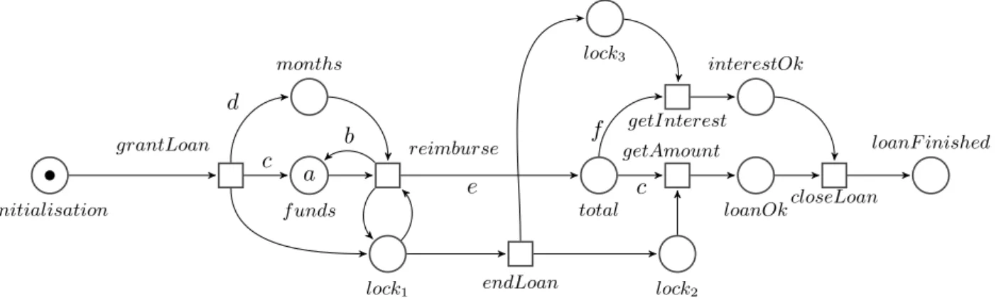
structure. We would like to provide a model allowing to model identical resources but also their synchronisation thanks to the paradigm of Petri nets. The formalism introduced in this thesis is not introduced in the aim to depict a precise case study. In this sense, we want to introduce a general purpose formalism. Nevertheless, we can guess that this increase in generecity will be gained at the cost of the complexity of the analysis. Moreover, we would like that the structure of the difference instances of the parameterised models keep the same structure in order to provide a quantitative analysis upon the valuations. Typically, a parameter can represent a number of processes but not only since we later provide an illustrative example by modelling a financial loan. In this context, we do not consider finite sets of valuation but infinite ones in order to study classic properties of Petri nets.

Close to our work, [Chiola et al., 1991] and [Marsan et al., 1994] present Petri Nets where the initial marking of the net can be parameterised. An initial marking with one or more parameters is an abstraction of a set of markings obtained by assigning different legal values to the parameters. We will prove in the sequel of this thesis that parameterising the markings can be simulated by parameterising the output weights. In a different manner, [Geeraerts et al., 2015] introduces Ê-Petri nets (ÊPN). This model augments classic Petri nets by allowing Ê-labelled input or output arcs. We will provide more details on this latest model in Section 3.5 since we will elaborate on some links with our model of parametric Petri nets and reuse some of the results proved for ÊPNs. The fundamental difference with our model is the non-determinism introduced by those labels. Indeed, an Ê-label input (resp. output) arc consumes (resp. produces), non-deterministically, any number of tokens in its input place (resp. output place). This model is said to be mainly used to analyse parametric concurrent systems with dynamic threads creation.

1.5 Contributions of this Thesis

As briefly mentioned earlier, RQ1is addressed by the introduction of the model of parametric

Petri nets (PPNs), aiming to represent families of concurrent systems. Discrete parameters are involved on the weight of arcs of the nets or in the initial marking. Moreover, syntactical subclasses are introduced in a matter of decidability and tractability. Parameters are restricted to initial markings only or weights of transitions only. In the latter case, we can impose that parameters on input arcs and output are distinct. Finally, we consider the case where parameters are used only as input weights or only as output weights.

To address RQ2, we consider the general property of coverability to which many safety

properties can be reduced and, to a lesser extent, boundedness and reachability (that are often the basis for the verification of more specific properties). This thesis dissertation deals with two decision problems induced by the use of parameters: The existential coverability: does there exists an integer valuation v on the set of parameters such that m is coverable in the marked Petri net where parameters are replaced by the value given by v? And the universal coverability: is m is coverable in such a net for every possible valuation v? Those problems are both undecidable in the most general case. Syntactic subclasses restricting the use of parameters have been introduced, for which the different problems are decidable and ExpSpace-complete. These results interestingly allows us to carry over a Rackoff upper bound into this parametric setting. Considering boundedness, we provide the result of decidability using some adaptations of the procedure of Karp and Miller for all those subclasses. We finally elaborate on decision frontiers by showing that the parametric reachability problems are undecidable for the subclasses of parametric Petri nets where parameters are used only on input arcs or only on output arcs, whereas it becomes decidable (for the existential problem) when parameters are used only on the initial marking. Note that the universal problem for this subclass is left open.

In order to address RQ3, we then focus on computing the exact solution set to the synthesis

problem for coverability in parametric Petri nets, i.e., the set of all parameter values such that in the net instantiated with these values, a given marking is coverable. The emptiness and universality of the solution set being undecidable in general, computing this set can only be

(22)

1.6. OUTLINE 21 done in a restricted setting. We thus focus on the case where parameters are used only as input weights (preT-PPNs) or only as output weights (postT-PPNs). These assumptions give some structure to the solution set: we prove that it is then downward-closed wrt. the usual order on integer vectors for preT-PPNs, and upward-closed for postT-PPNs. We show how a procedure by Valk and Jantzen from [Valk and Jantzen, 1985] can be used for computing a finite minimal basis of the solution set for postT-PPNs or its complement for preT-PPNs. This requires deciding universal coverability in preT-PPNs and existential coverability in postT-PPNs. Finally, we prove that in what will be called distinctT-PPNs, i.e., when the set of parameters appearing as input weights, and the set of parameters appearing as output weights are disjoint, the solution set cannot be represented using any formalism for which the emptiness of the intersection with equality constraints is decidable.

Those different results have been published in international conferences. The introduction of the model and some proofs of decidability have been first presented in a workshop [David et al., 2015b] and then have been published in [David et al., 2015a]. The work on complexities and synthesis has been accepted and will be published in [David et al., 2017].

1.6 Outline

All those results are presented in this thesis dissertation according to the following outline. Chapter 2 gives basic notations and recalls useful mathematical results from different theo-ries.

Chapter 3 reviews some elements of the state of the art regarding Petri nets, related decision problems and the classic procedure of Karp and Miller together with the model of Ê-Petri nets. Chapter 4 gives the basic definitions related to the formalism of parametric Petri nets, introduces two instances of decidability problems in parametric Petri nets, the universal and the existential instances, based on the definitions of classic properties of Petri nets. We also present the problem of the synthesis. We then provide a proof of the undecidability results of existential and universal coverability. Therefore, we refine the hierarchy of PPN to provide subclasses where universal or existential coverability are decidable.

Chapter 5 introduces these subclasses of our parameterised models and presents results of translation and monotonicity. We carry out a complete survey of decidability of parametric coverability in this restricted parametric setting with the corresponding complexities. We no-tably give constructions for proving the ExpSpace-completeness of the universal coverability for preT-PPNs. We then turn our attention to the problem of the synthesis.

In Chapter 6, we study the structure of the solution sets for preT-PPNs and postT-PPNs and show under which condition Valk and Jantzen’s algorithm can be used to construct finite representation of those sets. To complete this study, we propose a direct synthesis algorithm for preT-PPNs. We also discuss the case of distinctT-PPNs.

In Chapter 7, we emancipate from the problem of the coverability in order to establish decision frontiers in this parametric settings by studying the problem of existential and universal reachability and proving their undecidability for the subclasses of preT-PPNs and postT-PPNs. Interestingly, existential reachability becomes decidable when we restrict the use of parameters to initial markings only. Note that the remaining problem of universal reachability in P-PPNs is still an open problem.

Chapter 8 and 9 respectively conclude this thesis dissertation and present directions for future work.

(23)

(24)

CHAPTER

2

Discrete Mathematical Background

“Everything has beauty, but not everyone sees it.”

— Confucius

2.1 Notions of Set Theory and Order Theory . . . 23 2.1.1 Set Theory . . . 23 2.1.2 Order Theory . . . 24 2.1.3 Deepening of the Order Theory . . . 26 2.2 Notions of Graph Theory, Algebra and Enumerative Combinatorics 27 2.2.1 Graph Theory . . . 27 2.2.2 Elementary Algebra . . . 28 2.2.3 Combinatorics . . . 29 2.3 Computability Theory . . . 29 2.3.1 Turing Machines . . . 29 2.3.2 Decision Problems and Decidability . . . 30 2.3.3 Computational Complexity . . . 30

This chapter reviews basic notions and definitions about discrete mathematics from the field of mathematical logic, set theory and graph theory, from algebra, order theory and combina-torics. We also recall the notion of upward and downward closed sets. Those notions will be mainly reused in the definitions of the following chapters and in the different proofs. Readers familiar with those fields may skip this chapter or do a cursory reading and come back when specific references are made.

2.1 Notions of Set Theory and Order Theory

2.1.1 Set Theory

We recall here classic notions and notations of the set theory in the classic form of Zermelo-Fraenkel with the axiom of choice.

Intuitively, a set is a collection of distinct objects. The empty set is denoted by ÿ, membership by œ, set inclusion by ™ whereas strict inclusion is denoted by µ. We denote set intersection by fl, set union by fi and \ is used to denote the set difference. We denote by Z the set of integers, and by N the set of natural numbers. We denote by Ê an arbitrary large number such that for each n œ N, n + Ê = Ê, Ê ≠ n = Ê, Ê Æ Ê and n < Ê. We denote by NÊ is the union N fi {Ê}.

Let X be a finite set. We denote by 2X the powerset of X, that is to say the set of all subsets

of X and by |X| the size of X. If X ™ Nk_{, ¬X denotes its complement in N}k_.

(25)

The Cartesian product of two sets A and B, denoted by A ◊ B, is the set of ordered pairs {(a, b) | a œ A, b œ B}. The Cartesian product can be generalised to the n-ary Cartesian product over n sets X1, . . . , Xn such that X1◊ · · · ◊ Xn= {(x1, . . . , xn) | ’1 Æ i Æ n, xi œ Xi}.

We define correspondences between two sets through the notion of relation:

Definition 1 : Binary relation

A binary relation R between two sets X and Y is a subset of X ◊ Y . Given (x, y) œ R we say that x is related to y by R, which is denoted by xRy. The domain of R, denoted by dom(R), is the set {x œ X | ÷y œ Y, (x, y) œ R}. The set Y is the co-domain of R whereas the image of R, denoted by im(R) is the set {y œ Y | ÷x œ X, (x, y) œ R}, that is to say the subset of the co-domain effectively reached.

We call the binary relation on X the binary relation between X and X itself. Given a binary relation R œ X ◊ Y , we define R≠1 _{as the subset of Y ◊ Y such that for all x œ X, for all y œ Y ,}

y_R≠1x iff xRy. Given a binary relation f œ X ◊ Y , f is a partial functioniff (x, y) œ f and (x, z) œ f implies that y = z. In this case, we can write equivalently (x, y) œ f or f(x) = y since there is no ambiguity and y is called the image of x by f. If dom(f) = X, f is said to be a (total) function, we write f : X æ Y . The set of all (total) functions from X to Y is written YX. In

the sequel we may use the term mapping to refer to a total function in order to emphasise that we establish a correspondence between elements in one set with elements in another set.

Given X and Y two sets, for any subset XÕ _{™ X and function f œ Y}X_{, we define the}

restriction f_|XÕ of f to XÕ as the unique function from XÕ to Y such that f_|XÕ(x) = f(x) for all

xœ XÕ_{. We extend this notation to sets of functions: given F ™ Y}X_{, F}

|XÕ denotes its projection

on XÕ _{that is to say F}

|XÕ = {f_|XÕ | f œ F }. We now consider two sets A and B such that

X = A fiB and AflB = ÿ, and functions g œ YAand h œ YB, we write g fih œ YX the function defined by (g fi h)|A = g and (g fi h)|B = h. We call g fi h the union of g and h.

Definition 2 : Sequence

A sequence is an enumerated collection of objects from a set A in which rep-etitions are allowed. Formally, it is a function fs : D æ A whose domain

D is a convex subset of the set of integers, i.e. ’i, j œ D with i Æ j, ’k œ N, i Æ k Æ j ∆ k œ D. For i œ D, the element associated to the index i, fs(i) is simply denoted by si, and the sequence itself is denoted by (sn)nœD or

simply (sn).

The length of a sequence |(sn)| correspond to the cardinal of D. If D is finite, (sn) is said

finite, if not, D is necessary countable, by convention we can thus define |sn| = Ê. Finally, we

denote () the empty sequence which has a length equal to zero. Let A be a set, we denote by Aú the set of all finite sequences of elements of A. In language theory, A is called alphabet and those sequences can be seen as words. In this context, the empty sequence () is often written ‘ and is called the empty word. Let w œ Aú _{be a finite sequence. We write |w| the length of w.}

Given a œ A, |w|a is the number of occurrences of a in w.

Given a finite sequence s = s1, s2, . . . , sn, we call every sequence t of the form s1, . . . , sm

with m Æ n a prefix of s. We write t ı s. Given L a language over the alphabet A, that is to say a subset of Aú_{, we denote by P ref(L) the prefix closure of the language L, i.e.}

P ref(L) =t_s_œL{t | t ı s}.

2.1.2 Order Theory

We now introduce formally the intuitive notion of order using binary relations. We first need to introduce some properties for relations.

(26)

2.1. NOTIONS OF SET THEORY AND ORDER THEORY 25

Definition 3 : Relation properties

Given a binary relation R on a set S we say that R is reflexive: ’x œ S, xRx

irreflexive: ’x œ S, ¬(xRx)

symmetric: ’x, y œ S, xRy … yRx asymmetric: ’x, y œ S, xRy ∆ ¬(yRx)

antisymmetric: ’x, y œ S, (xRy · yRx) ∆ x = y transitive: ’x, y, z œ S, (xRy · yRz) ∆ xRz total: ’x, y œ S, xRy ‚ yRx

Given a binary relation R on a set X, the transitive closure of R written R+ _{is the minimal}

transitive relation on X that contains R. The reflexive transitive closure of R, written Rú_{, is}

the minimal transitive and reflexive relation on X that contains R. Based on those properties we now formalise the notion of order.

Definition 4 : Quasi order

A relation R that is reflexive and transitive is said to be a quasi order (qo for short).

A pair (S, .) is a quasiordered set if . is a quasiorder on S. Note that for the sequel, we use Æ when the relation is antisymmetric and . when it is not. For x and y elements of S and given a qo R on S, x and y are said comparable if either (x, y) œ R or (y, x) œ R. A relation < is a strict order on a set S if it is irreflexive and transitive (which implies asymmetry). A relation ≥ is an equivalence relation on a set S if it is reflexive, symmetric and transitive. Given any quasi order . on a set S we can define: (i) a strict order < given by x < y iff x . y · ¬(y . x), (ii) an equivalence relation ≥ given by x ≥ y iff x . y · y . x, (iii) its dual quasi order & given by y & x iff x . y.

Definition 5 : Well quasi order (See, e.g., [Higman, 1952] and [Kruskal, 1972])

A well quasi-ordering (wqo for short) is a qo . on a set S such that, for any infinite sequence s = x0, x1, x2, ... in S, there are indices i < j with xi. xj.

Let us also recall the following property:

Lemma 1

Given a set S and a well quasi order . on this set, let p0, p1, ..., pn, ... be

an infinite sequence of elements of S. Then, there is an infinite sequence pi1, pi2, ..., pin, ... such that pi1 . pi2 . ... . pin . .... (with i1< i2 <· · · < in<

. . .).

This can be easily understood using a Ramsey argument as follows: consider the set I = {i | there exists no j s.t. i < j and pi Æ pj}. If I were infinite, then we could extract a subsequence

of the terms indexed by the elements of I which would contradict the definition of wqo. Therefore I is finite. We can thus consider any pn with n greater than the maximal element of I as the

first element of such an infinite increasing subsequence. By construction of n and since N \ I is infinite, we can find an element m > n such that m ”œ I and pnÆ pm. We can thus iterate the

process and build a sequence satisfying the previous property.

Note that well quasi-orders can be defined in a various but equivalent manner, by ensuring that there exists no infinite strictly decreasing sequence (which is equivalent to a property called well foundedness) and that there is no infinite antichains (sequences of pairwise incomparable elements).

(27)

(S, =) where S is a finite set equipped with the equality relation on its elements (N, Æ), the set of natural numbers with standard ordering is a wqo (which is total). (Nk_,_{Æ) where Æ is the qo on N}k component-wise (this is known as the Dickson’s

lemma [Dickson, 1913] recalled below) (Nk

Ê,Æ) where Æ is the qo on NkÊ component-wise Lemma 2 : Dickson’s lemma [Dickson, 1913]

(Nk_,_{Æ), the set of vectors of k natural numbers with component-wise ordering,}

i.e. given two vectors m1 and m2, m1 Æ m2 if for all indexes i, m1(i) Æ m2(i),

is a wqo.

2.1.3 Deepening of the Order Theory

We reuse definitions and concepts from [Finkel and Goubault-Larrecq, 2009, Finkel and Goubault-Larrecq, 2012] which are summed up in [Finkel and Leroux, 2015].

Upward Closed Sets

An upward closed set of the well quasi ordered set (Nk_,_{Æ) is a subset U of N}k such that if

x _{œ U, y œ N}k _{and x Æ y then y œ U. The upward closure of a vector u, written ø u is the}

set {m œ Nk _{| u Æ m}. Given a set U, we write ø U for the upward closure of U, defined as}

ø U = tuœU ø u. This implies that ø U is the least upward closed set in which U is included.

Any upward closed set U can be represented by a finite set F , called basis, such that U =ø F. An element x of F is called minimal when for all element y œ F such that y Æ x, then x Æ y. The set of all the minimal elements of F ™ Nk _{still form a basis of U independently of F . This}

basis is minimal for inclusion among all bases and is thus called the minimal upward basis of F .

Downward Closed Sets

A downward closed set of the well quasi ordered set (Nk_,_{Æ) is a subset D of N}k _{such that}

if x œ D, y œ Nk and y Æ x then y œ D. The downward closure of a vector d, written ¿ d is

the set {m œ Nk _{| m Æ d}. Given a set D, we write ¿ D the downward closure of D, defined as}

¿ D =tdœD ¿ d. This implies that ¿ D is the least downward closed set in which D is included.

Moreover, the downward closure of a finite set (of vectors in Nk) is finite. To symbolically

represent downward closed sets, we use the extension Nk

Ê. The definitions remain otherwise the

same. If D is a downward closed set, we can write D = Nk_{ﬂ ¿ F where F is a finite set of N}k Ê.

We call F a downward basis of D. An element x of F is called maximal when for all element yœ F such that x Æ y, then y Æ x. The set of all maximal elements of F ™ Nk_{still form a basis}

of D independently of F . This basis is minimal for the inclusion among all bases and is thus called the minimal downward basis of D.

Some Notable Properties

We also recall important results on upward and downward closed sets (see, e.g., [Bouajjani and Mayr, 1999]): the union and the intersection of two upward (resp. downward) closed sets is an upward (resp. downward) closed set. The complement of an upward closed set is a downward closed set and vice-versa. Given the basis of an upward closed set, it is possible to compute the basis of its complement using for instance the procedure suggested in Example 5 of [Goubault-Larrecq, 2009], and vice versa by adapting this procedure.

Let us recall those procedures. First, we recall the reasoning of [Goubault-Larrecq, 2009]. This report provides as an example that the complement of ø(1, 3, 2) is exactly the intersection N3ﬂ ¿ {(0, Ê, Ê), (Ê, 2, Ê), (Ê, Ê, 1)}. Indeed, not being greater than or equal to (1, 3, 2) means

(28)

2.2. NOTIONS OF GRAPH THEORY, ALGEBRA AND ENUMERATIVE COMBINATORICS27 exactly having the first component less than or equal to 0, or the second component less than or equal to 2, or the third complement less than or equal to 1.

For the general case, given a vector x = (i1, i2, . . . , ik) the complement of øx in Nk is equal

to Nk_{ﬂ ¿{(Ê, . . . , Ê, i}

j≠ 1, Ê, . . . , Ê) | 1 Æ j Æ k, ij Ø 1}. Now if we consider a family of vectors

{x1, . . . , xm}, the complement of ø {x1, . . . , xm} can then be computed as the intersection of

the complements of ø x1, . . . ,ø xm. Moreover, we can notice that the following intersection

¿ {y1, . . . , ym}ﬂ ¿ {z1, . . . , zp} can be computed as ¿ {min(yi, zj) | 1 Æ i Æ m, 1 Æ j Æ p},

where min(yi, zj) are computed component-wise, for instance min((1, Ê, 3, Ê, 2), (3, 5, 0, Ê, Ê)) =

(1, 5, 0, Ê, 2).

Conversely, we can adapt this reasoning as follows: the complement of ¿ (Ê, 3, 2) is exactly N3ﬂ ø{(0, 4, 0), (0, 0, 3)}. Indeed, not being lower than or equal to (Ê, 3, 2) means exactly having the first component greater than Ê which is not possible, or the second component greater than or equal to 4, or the third complement greater than or equal to 3.

For the general case, given a vector x = (i1, i2, . . . , ik) the complement of ¿x in Nk is equal

to Nk_{ﬂ ø {(0, . . . , 0, i}

j+ 1, 0, . . . , 0) | 1 Æ j Æ k, ij ”= Ê}. Now if we consider a family of vectors

{x1, . . . , xm}, the complement of ¿ {x1, . . . , xm} can then be computed as the intersection of

the complements of ¿ x1, . . . ,_{¿ x}m. Moreover, we can notice that the following intersection

ø {y1, . . . , ym}ﬂ ø {z1, . . . , zp} can be computed as ø {max(yi, zj) | 1 Æ i Æ m, 1 Æ j Æ p},

where max(yi, zj) are computed component-wise, for instance max((1, Ê, 3, Ê, 2), (3, 5, 0, Ê, Ê)) =

(3, Ê, 3, Ê, Ê).

Finally, Valk and Jantzen proposed in [Valk and Jantzen, 1985] a necessary and sufficient condition, recalled in Lemma 3, to ensure that a finite basis of an upward closed set is effectively computable.

Lemma 3 : [Valk and Jantzen, 1985]

Given an upward closed set U ™ Nk, a finite basis of U is effectively computable

iff for each v œ Nk

Ê, the emptiness of ¿vﬂU is decidable, which is also equivalent

to ask whether for all element v œ Nk

Ê, it is decidable to answer whether ¿vﬂNk™

¬U.

2.2 Notions of Graph Theory, Algebra and Enumerative Combinatorics

2.2.1 Graph Theory

We now consider a set and a binary relation over itself. This pair of elements forms a directed graph.

Definition 6 : Directed graph

A directed graph G is a pair (V, A) where V is a set of vertices and A ™ V ◊ V is a set of pairs of vertices, called arcs.

In graph theory, it can be relevant to consider graphs where the nodes can be of different kinds. When vertices can be divided into two disjoint sets U and V, such that no arc relates two vertices from the same set, we can refine the above definition:

Definition 7 : Bipartite directed graph

A bipartite directed graph G is a triplet (U, V, A) where U and V are two disjoints sets of vertices and A ™ (U ◊ V ) ﬁ (V ◊ U) is a set of pairs of vertices, called arcs.

(29)

Definition 8 : Path

Given a directed graph G = (V, A) and n œ N, A path w : {1, . . . , n} æ V is a finite sequence of nodes such that ’i œ {1, . . . , n ≠ 1}, (w(i), w(i + 1)) œ A. We define a rooted tree as a triplet (T, r, S) where:

S _{™ T ◊ T , r œ T is the root, and for all t œ T , rS}út (with Sú the reflexive transitive closure of S)

’t œ T , t ”= r ∆ ÷ a unique tÕ œ T s.t. tÕSt

’t œ T , ¬(tS+t) (with S+ the transitive closure of S)

Informally, it is a directed graph where any two vertices are connected by one path and every arc can be assigned a natural orientation away from one given vertex (the root). We call the depth of a node the length of a path from the root to this node. By convention, the depth of the root is thus equal to zero.

Lemma 4 : König infinity lemma

Let T be a rooted (directed) tree in which each vertex has a finite number of successors (finite branching) and there is no infinite path directed away from the root. Then T is finite.

Each of those structures can be augmented by labelling functions assigning to each vertex or each arc an object.

We consider two alphabets 1 and 2. We consider a labelled tree defined as a graph by

a tuple C = (N, r, B, , ) where (N, r, B) is a rooted tree, : N æ 1 labels nodes with 1,

and : B æ 2 labels arcs with 2. We say that x is an ancestor of y iff (x, y) œ B+ where

B+ is the transitive closure of the relation B. Then, given a node n œ N, AncestorC(n), is the

set of ancestors of n in C plus n itself. Given two nodes x and y such that x œ AncestorC(y),

we write x y to denote the unique sequence of nodes along the path from x to y, that is to say x = n0, n1, . . . , nk = y such that each (ni, ni+1) œ B. We denote by pathC(x, y) œ Bú the

sequence of edges leading from x to y, formally it is equal to (n0, n1), (n1, n2), . . . , (nk≠1, nk). The

corresponding label is given by pathlabel_C(x, y) œ ú2. Given two trees T1= (N1, r1, B1, 1, 1)

and T2 = (N2, r2, B2, 2, 2), a mapping „ from N1 to N2 is a labelled tree isomorphism iff

„maps the root of T1 to the root of T2 i.e. „(r1) = r2.

’(u, v) œ N1, (u, v) œ B1… („(u), „(v)) œ B2 with 1(u, v) = 2(„(u), „(v))

for every node n of N1, 1(n) = 2(„(n)).

Given a tree C = (N, r, B, , ), CÕ _{= (N}Õ _{™ N, r}Õ_{, B}Õ _{™ B,} Õ_, Õ_{) is a prefix of C iff for each}

y œ NÕ_{, either y = r = r}Õ _{or if there exists a node x œ N such that (x, y) œ B then x œ N}Õ _and

(x, y) œ BÕ_{. Note that C}Õ _{is indeed a tree and that} Õ _and Õ _{are respectively the restrictions of}

and to NÕ _{and B}Õ_.

2.2.2 Elementary Algebra

Given a set of variables X, we define a linear expression on X by the following grammar: ⁄::= k | k ú x | ⁄ + ⁄ where k œ Z and x œ X.

Let V ™ NÊ, a V-valuation for X is a function from X to V . We refer to NÊ-valuations as

extended valuations and to N-valuations simply as valuations. The set Vÿ _{of valuations from ÿ}

to V is reduced to a singleton {ÿV} where ÿV is the empty function. If X is finite, considering

some arbitrary order on X, an (extended) valuation can be seen as a vector of size |X|.

Given a value a of NÊ, we denote as ˛a the uniform (extended) valuation that maps every

element of X to a. Given an extended valuation v, we write Ê(v) for the subset of X such that xœ Ê(v) iff v(x) = Ê. We write N(v) for the subset of X such that x œ N(v) iff v(x) œ N.

Given a linear expression ⁄ on X and an extended valuation v on XÕ _{™ X, v(⁄) is the linear}

expression obtained when substituting each element x in XÕ _{from ⁄, by the corresponding value}

(30)

2.3. COMPUTABILITY THEORY 29

2.2.3 Combinatorics

Given a function f : X æ Y , f is said to be injective iff given two elements x and xÕ _of

X, f(x) = f(xÕ) implies that x = xÕ. That is to say that f never maps distinct elements of its domain to the same element of its co-domain. Note that given x in X, y = f(x), when f is injective, x is called the fiber of y by f.

A function f is said to be surjective iff for every y of Y , there exists x œ X such that y= f(x). That is to say that the image of f is equal to its co-domain.

If f is both injective and surjective, f is said bijective. Informally, this means that the elements from the domain and the codomain of f are in one to one correspondence by f. Given a finite set X, we call the bijections (necessarily total) from X to X permutations.

Given a finite set X, SX denotes the symmetric group on X (i.e. the set of all permutations

of elements of X). If X is finite such that |X|=n, SX is finite and contains n! elements where

n! denotes the factorial of n. The notion of permutation is related to the act of arranging all the members of a set into some sequence or order, or if the set is already ordered, reordering its elements.

We also recall a well known result usually attributed to Dirichlet as the Dirichlet’s drawer principle but more commonly referred to as the pigeonhole principle.

Lemma 5 : Pigeonhole principle

There does not exist an injective function whose co-domain is smaller than its domain.

If n items are put into m containers, with n > m, then at least one container must contain more than one item. By extension, if n is infinite, then at least one container contains an infinity of items. Thus, if n = Ê, at least one container contains Ê items.

Numerous proofs will rely on this principle.

2.3 Computability Theory

Computability theory is a branch of mathematical logic and theory of computation. This theory notably addresses the notion of computable sets. We turn our interest toward decidability of decision problems in the sense originally introduced through [Turing, 1937].

2.3.1 Turing Machines

A Turing machine is a theoretical machine that reads and write symbols one at a time at a position given by the head of the machine which moves on the cells of an infinite tape by following a program. Let us provide a formal definition. Given an alphabet A we define ˜A = A ﬁ {⇤} where ⇤ will be used to represent an empty cell from the tape.

Definition 9 : Turing Machine

A Turing machine on an alphabet A is a pair (Q, æ) such that:

Q is a set of states containing at least the initial state init, the accepting state accept and the rejecting state reject

æ™ Q ◊ ˜A◊ ˜A◊ {≠1, 0, +1} ◊ Q is the transition relation

We define the configuration of a Turing machine as a triplet (q, f, i) where q œ Q, f : Z æ ˜A represents the contents of the tape and i œ Z represents the current position of the head. The initial configuration defined on the input w is the triplet (init, f0,0) where for 0 Æ i Æ |w| ≠ 1, f₀(i) = w(i) and f(i) = ⇤ otherwise.

Given a Turing machine, its configuration (q, f, i) yields in one step the configuration (qÕ_{, f}Õ_{, i}Õ_{) iff ÷(q, a, b, x, q}Õ_{) œæ such that:}

(31)

a= f(i) (i.e. the head reads a on the tape) b= fÕ(i) (i.e. the head writes b on the tape) ’j ”= i, fÕ_{(j) = f(j)}

iÕ = i + x

Given a configuration if there is only one transition yielding another configuration, the machine is said deterministic. Otherwise it is said non-deterministic. Given an input w, if the machine reaches the state accept the machine stops and return true and if the machine reaches the state reject the machine stops and return false.

2.3.2 Decision Problems and Decidability

In computer science, a problem is characterised by a set of input instances and a task to perform on these input instances. The problem is encoded into a specialised format for efficient transmission, storage or processing by the machine.

A decision problem is a question which can be answered by a Boolean value depending on the input values. Note that the set of possible input values may be infinite. For instance asking whether an integer n œ N is a prime number is a decision problem. A decision problem can be assimilated to the set of possible inputs, called solution set, for which the answer is true.

A decision problem is said decidable iff there exists an algorithm which terminates after a finite amount of time (which may depend on the input value) and correctly decides whether the input is in the solution set or not. It is semi-decidable if there exists an algorithm that correctly decides when an input is in the solution set but may give no answer (i.e. may not terminate) for input not in the solution set. A problem that is not decidable is called undecidable. Note that some examples of decidable decision problems are presented in the next chapter when introducing the background on Petri nets, more precisely in Section 3.2.

In order to formalise the notion algorithm we need to rely on a specific formal model of computation. In particular we use here the formal model of Turing machine presented above. Indeed, any Turing machine can be translated in an effective algorithm. This means that every problem that is decidable through a Turing machine is decidable through an algorithm. Reciprocally, we admit that the decidability of a problem implies its decidability through a Turing machine. This latter implication is often referred to as the Church-Turing thesis.

Therefore, the definition of decidability is equivalent to the existence of a Turing machine which terminates after a finite number of steps (which may depend on the input value) and correctly decides whether the input is in the solution set or not.

2.3.3 Computational Complexity

We now focus on classifying decidable problems according to their difficulty by formalising that for a given problem, finding its solution requires a certain amount of resources, whatever the algorithm used. In particular, in this section, we provide the definition of the class ExpSpace since the majority of the results proved in this manuscript belong to it.

To quantify the amount of resources needed, we refer to the Turing machines: if we consider decidable problems, we can deduce that there exists a Turing machine solving any instance of this problem, this instance being the input of the machine. Based on this observation, we define the complexity in time as the number of steps performed by the machine to stop (which might depend on the encoding). We also define the complexity in space as the maximal number of cells used (i.e. containing a element of the alphabet different from ⇤) by the machine along its execution, from the beginning until the termination.

Given two functions f, g : N æ N, we compare the asymptotic behaviour of f and g by writing that g(n) = O(f(n)) when n increases toward infinity which means that there exists some constants c œ R+_{, the set of positive real numbers, and N œ N such that for all n Ø N,}

(32)

2.3. COMPUTABILITY THEORY 31 of size n. We denote the asymptotic complexity of a Turing machine by O(f(n)) according to the previous definition.

The class ExpSpace is the set of all decision problems solvable by a deterministic Turing machine in O(2p(n)_{) space, where p(n) is a polynomial function of n. The class NExpSpace is}

the set of all decision problems solvable by a non-deterministic Turing machine in O(2p(n)_{) space,}

where p(n) is a polynomial function of n. Those two classes are known to be equal:

Corollary 6 : Corollary of Savitch’s theorem [Savitch, 1970]

NExpSpace is equal to ExpSpace.

A decision problem is ExpSpace-complete if it is in ExpSpace, and every problem in ExpSpace has a time reduction to it. That is to say that there is a polynomial-time1_{algorithm that transforms instances of one to instances of the other with the same answer.}

Intuitively, it means that the complexity has an ExpSpace upper bound and that it is as hard as any ExpSpace problem which provides a lower bound. This lower bound is referred to as ExpSpace-hardness.

We provided an extensive list of mathematical notions and background notations used throughout this thesis dissertation. We are now in position to introduce elements of the state of the art regarding Petri Nets which will be done in the following chapter.

1. An algorithm is said to be polynomial-time (or to have a polynomial running time) if there exists k œ N and C > 0 such that given any input of size n its running time is at most Cnk_.

(33)

(34)

CHAPTER

3

Preliminaries on Petri Nets

“Those who do not want to imitate anything, produce nothing.”

— Salavador Dali

3.1 Definitions and Examples . . . 33 3.1.1 Formal Definition . . . 33 3.1.2 Operational Semantics . . . 34 3.1.3 Well Structured Transition Systems . . . 35 3.1.4 Equivalent Modelling Formalism . . . 35 3.2 Behavioural Properties of Petri Nets . . . 36 3.3 Analysis of Petri Nets . . . 38 3.3.1 Existence of Self-Covering Sequences . . . 38 3.3.2 Karp and Miller Procedure . . . 39 3.3.3 Introduction to the Rackoff Upperbound . . . 40 3.4 Simulations of Nets . . . 41 3.5 Notable Petri Nets Extensions . . . 42

This chapter intends to introduce Petri nets in such a way that only classic properties and results are presented. Those results will be extended to a parametric context in the following chapters. Petri nets (or place/transition net) are a basic model of parallel and distributed systems introduced by Carl Adam Petri [Petri, 1962]. Petri nets are designed to model discrete event systems by exhibiting behaviours such as concurrency, conflict or dependency between events in both a graphical and formal manner through a strong mathematical background.

3.1 Definitions and Examples

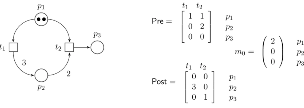
3.1.1 Formal Definition

A Petri net is a bipartite graph consisting of places, transitions and arcs. An example is provided in Figure 3.1. Transitions represent events that may occur, they are depicted by squares (or sometimes bars in the literature). Places represent conditions, they are depicted by circles.