Critical points and reaction paths characterization on a potential
energy hypersurface
Marie-Noe¨lle Ramquet, Georges Dive,a) and Dominique Dehareng Centre d’Inge´nierie des Prote´ines, Universite´ de Lie`ge, Institut de Chimie B6, Sart-Tilman, B-4000 Lie`ge, Belgium
共Received 7 April 1999; accepted 21 December 1999兲
Most of the time, the definitions of minima, saddle points or more generally order p ( p
⫽0, . . . ,n) critical points, do not mention the possibility of having zero Hessian eigenvalues. This
feature reflects some flatness of the potential energy hypersurface in a special eigendirection which is not often taken into account. Thus, the definitions of critical points are revisited in a more general framework within this context. The concepts of bifurcation points, branching points, and valley ridge inflection points are investigated. New definitions based on the mathematical formulation of the reaction path are given and some of their properties are outlined. © 2000 American Institute
of Physics.关S0021-9606共00兲01110-7兴
I. INTRODUCTION
In order to explore a potential energy surface, the first step is usually to locate and characterize the minima and saddle points. The surface dimension is given by the number of degrees of freedom of the molecular system and is equal to 3N⫺6 where N is the number of atoms. Most of the time, since this dimension is high and since the energy function has to be computed numerically point by point, the knowl-edge of the potential energy surface is often limited to some local regions of chemical interest. Minima are stable equilib-rium points and thus they represent the initial and final states of the transformation process. From their nature, saddle points are unstable equilibrium points and are associated with transition state structures. Minima and saddle points still have a common property: They are stationary points of the energy function. To differentiate or characterize them, Mezey,1 Mu¨ller2 and Schlegel3 base their reasoning on the Hessian eigenvalue spectrum. But vanishing Hessian eigen-values is not often mentioned. Zero local conical curvatures are present at the boundaries of curvature-based topologies of potential energy hypersurfaces. They are the subject of extensive works by Mezey.4–6He also details various cases of stationary points with zero Hessian eigenvalues.7
Except within the framework of symmetry, exact zero eigenvalues rarely occur. Nevertheless some potential energy surfaces are so flat that the Hessian eigenvalues are very small in magnitude. Moreover, because the gradient never reaches zero numerically, the flatness zone looks like a sta-tionary region. This situation can be encountered for weak complexes. The problem of Jahn–Teller 共and related兲 ef-fect共s兲 will not be considered here because this implies nona-diabatic coupling between two or more electronic states. In this framework, the derivation of the energy, the gradient, and the Hessian is questionable. In this work, we are dealing
with only one well-defined energy surface quite decoupled from any other one.
After locating and characterizing stationary points, it is often useful to check that a particular transition state 共TS兲 connects the desired minima. This can be done by computing the reaction path8–10 that is the union of the two steepest descent energy paths going down the potential energy sur-face from the TS to the adjacent minima.
Nevertheless lots of potential energy surfaces seem to possess points where the reaction path bifurcates, splits it-self, crosses one or more 共equivalent兲 paths or simply be-comes unstable. These notions have partially been studied in the literature by Baker,11 Bosh,12 Schlegel13 and Valtazanos.14 They have defined some special points as bi-furcation points or branching points. Valley ridge inflection points共VRI兲, which are very unstable points along the reac-tion path, are also evoked in these papers. Most of the time, the definitions given for these concepts differ and are some-times incompatible. Baker11 and Bosh12 do not mention the necessity of having a vanishing gradient. But Valtazanos14 shows that the steepest descent path共SDP兲 will never bifur-cate at a nonstationary point and consequently the SDP is not suitable for studying a reaction path. They also state that in general there exist no orthogonal trajectory patterns which could serve as simplified models for channel bifurcations. Bosh12suggests constructing an alternative route that follows the valley, not the ridge.
In an algorithmical point of view, when computing a reaction path, the calculated points never coincide exactly with the path describing the motion of the molecules or wave packets on the potential energy hypersurface. Thus when passing through or near a zone of instability and in particular a VRI, the computed path may split in two or deviate even if in theory, the SDP does not. Considering the evolution of a wave packet along a SDP, its lateral points will follow dis-tinct SDP, and near a VRI, the wave packet could split. Moreover following Taketsugu,15since the reaction path
ob-a兲Author to whom correspondence should be addressed; electronic mail: [email protected]
JOURNAL OF CHEMICAL PHYSICS VOLUME 112, NUMBER 11 15 MARCH 2000
4923
viously exists with its complementary vibrational motions, the reaction channel must bifurcate at the VRI.
The first aim of the present paper is to formulate new definitions for these particular regions near the reaction path and outline their properties in the framework of a more gen-eral definition of order p ( p⫽0, . . . ,n) critical points. The second purpose of this work is to include in this general definition the occurrence of null Hessian eigenvalues.
II. DEFINITIONS
In the Born–Oppenheimer approximation,16 a unique potential energy surface共PES兲 may be assigned to any elec-tronic state of a given molecule. Within this context, the function describing this hypersurface is denoted E and de-pends on the nuclear coordinates. This is a well-defined and well-behaved function for most points ofRnexcept for those corresponding to configurations where some nuclei occupy
the same position. We then may assume that there exists an open subset of Rn, ⍀, wherein E is at least twice continu-ously differentiable. This assumption is necessary since most processes for exploring a PES are based on the location of its stationary points and rely on the continuous differentiability of the gradient of E. So E may be approximated by a Taylor expansion, i.e.,
᭙x0苸⍀,E共x0⫹D兲⬵E共x0兲⫹G˜共x0兲D⫹1
2D˜ H共x0兲D, 共2.1兲
where G(x0) is the gradient vector of E at x0, G˜ (x0) its
transposed, and关G(x0)兴i⫽(E/xi) (x0), similarly H(x0) is
the Hessian matrix of E at x0, and 关H(x0)兴i, j
⫽(2E/x
ixj) (x0), D苸Rn½, D⬇0.
By definition,17 x0 is a minimum if and only if
᭚⬎0:᭙D苸Rn½:兩D兩⬍, f共x0⫹D兲⭓ f共x0兲 共2.2兲 and x0 is a saddle point if and only if
᭚D,⬎0:᭙兩兩⬍,
再
f共x0⫹D兲⭐ f共x0兲f共x0⫹D⬜兲⭓ f 共x0兲᭙D⬜⬜D, 兩D⬜兩⫽兩D兩. 共2.3兲
More generally, x0 will be defined as a critical point of order p ( p⫽0, . . . ,n) if and only if ᭚D1⬜ . . .⬜Dp,⬎0:᭙兩兩⬍,
再
f共x0⫹Di兲⭐ f 共x0兲, 共i⫽1, . . . ,p兲
f共x0⫹D⬜兲⭓ f 共x0兲᭙D⬜⬜Di, 兩D⬜兩⫽兩Di兩, 共i⫽1, . . . ,p兲.
共2.4兲
This means that at a minimum, the energy function is minimum in all directions of Rn½ and at a saddle point, the energy function is maximum along one direction and mini-mal in all orthogonal directions. More generally, a critical point of order p ( p⫽0, . . . ,n) is a point at which the energy function is maximal along p directions mutually orthogonal and minimal along n – p directions orthogonal to each other and to the first p ones. The case where p⫽0 corresponds to a minimum. Mu¨ller2 and Schlegel3,18 introduce minima, saddle points, and critical points of various order in this way. According to a general mathematical terminology, the order of a critical point of a one dimensional function is determined by the first nonvanishing derivative while the index of a critical point is given by the number of strictly negative Hessian eigenvalues. For example, 0 is a fourth order critical point for the function f :R→R:x哫x4 and (0,0) is of index 1 for the function f :R2→R:(x,y)哫x2⫺y2.
Most of the time, the ‘‘order’’ of the critical point as defined by Eq.共2.4兲 is given by the Hessian eigenvalue spec-trum and usually corresponds to the index. The quantity p used in this paper is not strictly the index but the number of orthogonal directions along which the critical point is a maximum for the function considered. These two quantities are identical when there are no vanishing Hessian eigenval-ues.
A. Characterization of critical points
If the Hessian eigenvalues of a critical point are all strictly positive, the point is a minimum. If, at a critical point
P, there are p ( p⫽0, . . . ,n) strictly negative Hessian eigen-values and n⫺p strictly positive ones, then P is a critical point of order p and in particular, when p⫽1, P is a saddle point. This criterion is sufficient but not necessary. If every stationary point with exactly p strictly negative Hessian ei-genvalues and n⫺p strictly positive ones is a critical point of order p, the converse is not true. Thus, a stationary point with a zero Hessian eigenvalue and n⫺1 strictly positive ones could either be a saddle point or a minimum. Consider the following functions f1:R2→R:(x,y)哫x2⫺y2, f2:R2
→R:(x,y)哫x2⫺y4 and f
3:R2→R:(x,y)哫x2⫹y4. Their
graphs are depicted in Figs. 1共a兲, 1共b兲, and 1共c兲, respectively. Figures 1共a兲 and 1共b兲 have similar shapes and from equalities 共2.2兲 and 共2.3兲, it can be proven that (0,0) is a saddle point in the first two cases and a minimum in the third one. The Hessian eigenvalues at (0,0) are (⫺2,2), (0,2), and (0,2). In the last two cases, the Hessian eigenvalue spectra are identical even if (0,0) is a saddle point for f2 and a
minimum for f3. This example confirms that a saddle point
could either be characterized by one strictly negative eigen-value and n⫺1 strictly positive ones or by q (q⫽0, . . . ,n) zero ones and n⫺q strictly positive ones.17This emphasizes that there is no simple definition of a critical point of order p based on its Hessian eigenvalue spectrum if there are zero eigenvalues and consequently that the notion of index is not sufficient. Thus the term ‘‘order’’ will be used within the framework of this paper as the number of orthogonal direc-tions along which the critical point is a maximum.
Vanishing Hessian eigenvalues simply indicate some flatness for the function graph. It is a local property and only concerns one single point, i.e., the stationary point. When vanishing eigenvalue共s兲 occur共s兲 at a critical point, a little
farther away from it, the zero Hessian eigenvalue共s兲 could turn to positive or negative and even could become very large. This is illustrated by Fig. 2. The function f is given in Ref. 19.
Figures 2共a兲 and 2共b兲 are two graphs of the function f at different scales. The point (0,0) is a critical point of order 1, i.e., a saddle point even if the Hessian eigenvalues at (0,0) are both zero. But a little bit away from it, the eigenvalues are, respectively, strictly positive and strictly negative and of large magnitude (兩vp1(0.01,0.01)兩⫽兩vp2(0.01,0.01)兩
⫽0.618194). Depending on the scaling view, the graph of
the function f looks like that of x2⫺y2 关Fig. 2共a兲兴 or x4
⫺y4 关Fig. 2共b兲兴. B. Reaction path
In any given coordinate system, the simplest method for following a reaction path from a saddle point associated with a TS down to the minima is to solve the differential equation
dx共s兲
ds ⫽⫺
G共x共s兲兲
储G共x共s兲兲储,
共2.5兲 FIG. 1. Graphics of共a兲 x2⫺y2,共b兲 x2⫺y4,共c兲 x2⫹y4. At the point (0,0),
the last two functions have the same eigenvalues spectrum and they are shaped like a transition state and a minimum, respectively.
FIG. 2. Graphic of the function given in Ref. 19 at two different scales,共a兲 in the interval 关⫺0.2,0.2兴⫻关⫺0.2,0.2兴 and 共b兲 in 关⫺0.02,0.02兴 ⫻关⫺0.02,0.02兴.
4925
x共s0兲⫽x0,
where 储•储 denotes the modulus and s plays the role of an arclength.20–22
This defines the SDP; if expressed in mass weighted cartesian coordinates, this path corresponds to the intrinsic reaction path共IRC兲.8This method is particularly useful if we want to go from a saddle point down to a minimum but is useless for going from below to above, i.e., for climbing along the PES. Steepest descent paths and their properties have been discussed by Mezey.7
This definition of the reaction path关Eq. 共2.5兲兴 no longer holds at stationary points since the gradient is null. The SDP is the unique solution of a Cauchy problem and is defined independently from the concepts of eigenvalues or eigenvec-tors. The approximated path is obtained on the basis of a second-order Taylor expansion of the energy function. In the case where there are zero eigenvalues at a stationary point, the numerical determination of the SDP requires higher order derivatives. One has to bear in mind the distinction between the analytical path, solution of Eq. 共2.5兲, and its numerical approximation.
III. BIFURCATION POINTS
A. Definition and properties of bifurcation points
In Sec. III A 1, we will recall the definitions given in the literature and investigate their limitations.
1. Point with one Hessian zero eigenvalue
Bosch et al.12 define special points called bifurcation or branching points as points on the IRC where the curvature changes from positive to negative. i.e., points at which the IRC changes from a stable valley to an unstable ridge. They characterize them as points at which the gradient of the en-ergy function does not necessarily vanish and where the Hes-sian matrix possesses one zero eigenvalue corresponding to a direction orthogonal to the tangent vector, i.e., to the vector
dx(s)/ds⫽⫺G(x(s))/储G(x(s))储. They propose a simple
method for stepping at the branching point to the SDP that follows the valley. But this definition is not sufficient. Con-sider the function f :R2→R:(x,y)→x4⫹(y⫺2)2⫹y. Its gradient is (4x3,2(y⫺2)⫹1) and the SDP passing through (0,2) is given by the unique solution of the differential equa-tion dx共s兲 ds ⫽⫺ 4x共s兲3
冑
16x共s兲6⫹共2y共s兲⫺3兲2 , d y共s兲 ds ⫽⫺ 2 y共s兲⫺3冑
16x共s兲6⫹共2y共s兲⫺3兲2 , x共0兲⫽0, y共0兲⫽2,and consequently the curve (x(s)⫽0, y(s)⫽s⫺2) is the SDP representing the reaction channel. Except for the sta-tionary point (0,3/2), every point of this path has a Hessian characterized by a zero eigenvalue relative to an eigenvector orthogonal to the path. They all satisfy the criteria introduced by Bosh even if no bifurcation occurs since the path (0,s
⫺2) is the only SDP passing through these points. However,
most papers11,12associating VRI with bifurcation points con-sider in a general sense the reaction channel or the valley path, but do not mention the steepest descent path.
A zero Hessian eigenvalue does not necessarily imply a bifurcation point and conversely, a bifurcation is not always associated with a zero Hessian eigenvalue. Consider the very well known function f (x,y )⫽x2⫺y2. The saddle point (0,0) can be seen as a bifurcation point since path共1兲 represents an IRC that splits at (0,0) into two new equivalent paths 关共2兲 and共3兲兴 even if no eigenvalue vanishes at (0,0) 共Fig. 3兲. In order for path共1兲 to be an IRC, 共1兲 must start from an addi-tional saddle point located above (0,0).
Such an example of saddle-to-saddle descent path has been presented theoretically by Mezey in his book7 and illustrated23 with the two-dimensional relaxed conforma-tional map involving the two C–O bond rotation angles of catechol.
2. Bifurcation points within the context of symmetry
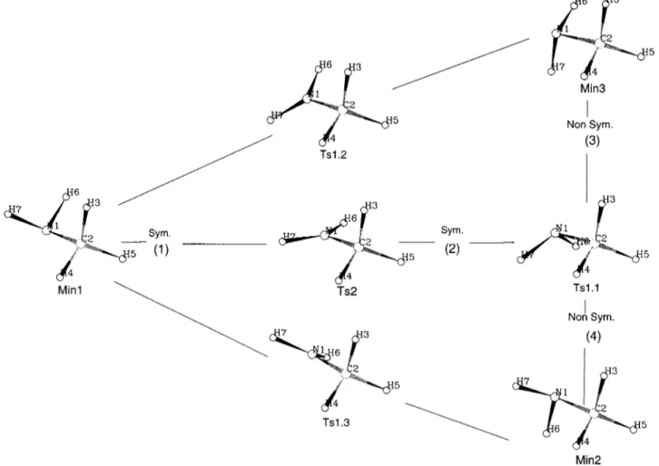
Bifurcations are often associated with symmetry break-ing. According to Baker et al.,11 a bifurcation point or a branching point can be considered as a point of the reaction path where it is energetically favorable to break out the sym-metry. But considering the methylamine PES24,25allows one to conclude that this point of view is not sufficient. Figure 4 is the geometrical diagram corresponding to the PES related to the internal rotation-nitrogen inversion.
Structures Min1, Min2, and Min3 are the minima, Ts1.1, Ts1.2, Ts1.3 are saddle points while Ts2 is a critical point of second order. Some of these paths are symmetry preserving
关共1兲 and 共2兲兴 while the others are not 关共3兲 and 共4兲兴. From this
point of view, Ts1.1 and Min1 are bifurcation points. But Min1 is a minimum and the question remains if it can really be treated as a bifurcation point. They are sometimes called ‘‘multibifurcation’’ points since they are the confluence of an infinity of SDP.14
3. Bifurcation points as stationary points
It has been proven26 that for the Cauchy problem 关Eq.
共2.5兲兴, if there exists an open subset ⍀ of Rn such that
共1兲 f :Rn→Rn:x哫 f (x) is once continuously differentiable,
FIG. 3. Illustration of a bifurcating reaction path on the surface generated by the function x2⫺y2关path 共1兲 splits into paths 共2兲 and 共3兲兴.
᭙x0苸⍀,᭚C1,C2:᭙x:d共x,x0兲⬍C1,
冐
冉
f共x兲 x1 , . . . ,f共x兲 xn冊
冐
⬍C2,共2兲 the differential of f, D f ⫽(f /x1, . . . ,f /xn) is locally bounded in ⍀, then the Cauchy problem is said to be well posed and through each point of⍀ passes exactly one regu-lar SDP curve. Thus, the Cauchy problem 关Eq. 共2.5兲兴 has exactly one solution x(s) defined on an interval I such that
共1兲 if x
⬘
(s) is another solution of the Cauchy problem de-fined on another interval I⬘
of R, then ᭙s苸I⬘
, x(s)⫽x⬘
(s) and I⬘
傺I, i.e., the Cauchy problem has exactly one maximal solution,共2兲 dx(s)/ds is continuous within the whole domain of the
definition of x(s).
Since the PES was assumed to be twice continuously differentiable, the function G(x)/储G(x)储 is continuously dif-ferentiable and locally bounded on the set ⍀
⫽兵x苸Rn:储G(x)储⫽0其. Consequently, at every nonstationary point of the PES passes exactly one SDP and the tangent vector is a continuous function (vTr⫽dx(s)/ds); conversely, if at a point of⍀ the path splits itself or if its tangent is not continuous then the point must be stationary.
Valtazanos14 has already stated that bifurcation of SDP occurs only at stationary points. He goes on to say that
be-cause of this property, SDPs are not suitable for studying the bifurcation of reaction channels. Some aspects and examples of bifurcating reaction paths have been given by Mezey.4,7
B. Analytical examples
With general analytical examples, we prove herein that the concept of bifurcation does not always have to be asso-ciated with Hessian zero eigenvalues. We first investigate C1
cases, i.e., situations without any particular symmetry and then a general symmetrical context.
1. General context without any symmetry
Figure 5 represents a part of a typical model reaction path. The bifurcation point X0 is stationary, the path joining the TS to X0 is denoted as 共1兲 and the two descent paths going down from X0 are 共2兲 and 共3兲.
共a兲 if the line formed by the two paths 共2兲 and 共3兲 was
not a broken line and formed one unique path, i.e., if the tangents to 共2兲 and 共3兲 (v and ⫺v兲 with the same modulus were parallel but had opposite orientations, then no Hessian vanishing eigenvalues would be necessary at X0.
共b兲 if 共2兲 and 共3兲 had different tangent (v and v
⬘
), i.e., if they referred to two different eigenvectors and they lead to two distinct regions of the configuration space, then there would have to be at least two orthogonal descent directionsFIG. 4. Schema of a part of the methylamine PES. Three minima共Min1, Min2, Min3兲 are connected to each other directly through three first-order critical points共Ts1.1, Ts1.2 and Ts1.3兲. Min1 and Min2 or Min1 and Min3 are connected indirectly through a unique second-order critical point 共Ts2兲.
4927
and consequently, at least two Hessian negative eigenvalues. Vanishing eigenvalues are not necessarily required.
These two examples point out that Hessian zero eigen-values are not always necessarily required for bifurcation or path division.
2. Particular case where there is some symmetry
In this section, the case where the chemical system has some symmetry is investigated. We recall that symmetry breaking while following a steepest descent path for a reac-tion process may only occur at a stareac-tionary point and that it brings path bifurcations.
Following Pearson,27if the symmetry is broken during a reaction process, a bifurcation must occur as there exist at least two products that are transformed into each other by some symmetry operation. Since bifurcations may only take place at stationary points, the symmetry loss may only occur at a critical point.
Mezey7 also proves that the nuclear symmetry is pre-served along SDPs between critical points. Moreover he shows that if the reactant and product configurations (C1and C2), respectively, are not related by symmetry, then the
symmetry group of the transition structure must belong to a
common subgroup of the symmetry subgroup of C1and C2.
Various symmetry related theorems are detailed by Mezey in Refs. 28–31.
Let x1, . . . ,xn be a complete coordinate system and
x1
⬘
, . . . ,xp⬘
( p⬍n) a coordinate system in a restrained sym-metrical context. The criterion is: a TS has the same order both in the complete coordinate system and in a symmetrical one if and only if no symmetry breaking happens. This can be intuitively understood from the following reasoning: If the orders of the stationary point in the two coordinate sys-tems were different, i.e., if the stationary point was a mini-mum in the symmetrical context and a first-order critical point in the complete coordinate system, then the SDP can-not continue in symmetrical coordinates since the path reached a minimum in this context. But, in the complete coordinate system, this path still has to carry on since it only reached a first-order critical point and thus, the path has to break the symmetry. Conversely, if the symmetry is broken, some ‘‘nonsymmetrical’’ variables must be involved in the tangent vector and thus the critical point cannot have the same order in a symmetrical or in a complete system of coordinates.This criterion could be used to locally reduce the dimen-sion of the hypersurface associated with a reaction process and consequently reduce its complexity by dealing with the significant degrees of freedom only and not with the redun-dant ones reflecting the symmetry.
When following a reaction path, special care must be taken in the detection of bifurcation points. When reaching a stationary point, it is necessary to check out its nature, i.e., its order. Special attention must be paid when dealing with Hessian zero eigenvalues since, if at a stationary point the smallest eigenvalue is zero, it may correspond to either a minimum or a saddle point. For recall 共Sec. II A兲 the func-tions x2⫹y4and x2⫺y4both have a zero Hessian eigenvalue and a positive one at (0,0) but in the first case, (0,0) is a minimum and in the second, a first-order critical point. If the Hessian is of full rank, the eigenvalues spectrum is sufficient to characterize the nature of the critical point but if the Hes-sian has zero eigenvalues, at least third order derivatives are required.
C. Chemical examples
To illustrate our considerations, we present two chemical examples already studied in the literature.
1. Isomerization of the methoxy radical
This example was studied earlier by Colwell et al.32and revisited by Baker et al.11 It describes the isomerization of the methoxy radical. The interesting part of PES for our pur-pose is shown schematically in Fig. 6. All the unrestricted Hartree–Fock calculations have been performed in a system of internal coordinates using the STO-3G basis set.
Structures I and V correspond to the minima, II and IV are transition states since they both have an imaginary fre-quency. At point III, the curvature along one direction dis-tinct from the SDP changes from positive to negative in the chosen system of internal coordinates and is a VRI. The solid curve linking I to IV through II is the minimum energy path
FIG. 5. Schematic illustrations of two paths bifurcating at a stationary point
x0:共a兲 the paths 共2兲 and 共3兲 have antiparallel tangents at x0;共b兲 at x0, paths
and is symmetry preserving. Then the channel divides itself into two equivalent branches leading respectively to V and
V
⬘
. This confirms that IV is a bifurcation point for which there are no vanishing Hessian eigenvalues. Obviously, this case of bifurcation is directly related to symmetry breaking since the reaction path leads to two structures that are trans-formed into each other by a reflection operation.Moreover this example shows us how important it is to locate as many stationary points as possible since if we omit point IV then the direct path 共III,V兲 could no longer be viewed as a SDP and consequently III would be considered as a bifurcation point instead of IV as in Baker’s model11 even if III is not a stationary point. Anyway III is surrounded by a very interesting region to investigate since it is very unstable. This point is studied in Sec. IV D.
2. Double sylation of ethylene
Let us now consider a second example that is the subject of a reaction path study by Raaii et al.33 Their reactional schema mentioned some saddle points, minima, and a bifur-cation point. Figure 7 shows some SDPs for the double sy-lation reaction of ethylene traced at the RHF/6-31G共d兲 level. Once stationary points were characterized as minima or higher order critical points, the IRCs were followed from each transition state down to the corresponding minima in internal coordinates with update of the Hessian at each step. This example involves some symmetry and bifurcation points. The interesting part of the reaction scheme has six critical points 共TS1, TS2, TS3, TS4, TS5.1, TS5.2兲 and two of them 共TS5.1 and TS5.2兲 are transformed into each other by a reflection operation. The second order critical point
共TS1兲 with Cs symmetry is connected via TS4 to the
mini-mum representing the products Gauche 1 and Gauche 2 that are transformed into each other by a reflection operation. These two conformers are also the endpoints of the IRC coming from TS3. Through the symmetrical TS5.1 and 5.2, the gauche minima generate the final trans structure that is a minimum. Raaii mentioned a hypothetical bifurcation point somewhere along the IRC going down from TS2. At this bifurcation point, the IRC had to split into two equivalent branches, one leading to Gauche 1 and the other one, leading to Gauche 2. Since it has been proven that bifurcations may only take place at stationary points, we propose that TS3 and TS4 are bifurcation points. From the context, these points have to be associated with symmetry breaking.
IV. ABOUT THE VRIs
If a SDP comes to a point where the followed valley turns into a ridge, then this point is called a VRI. Such points have often been confused with bifurcation points since the region around them is unstable. When computing the path, if the actual calculated path deviates slightly from its theoreti-cally correct route, it can diverge strongly. How fast a SDP deviates from the ridge depends on the stability of the nu-merical algorithm. For integrating differential equations, im-plicit algorithms are much more stable than exim-plicit ones. Nevertheless, their formulation involves some circular refer-ences and they are more difficult to implement into numeri-cal programs.
Most of the time, VRIs have been studied in the context of symmetry11,14,34but as previously, our consideration will hold within a more general framework. The following
ex-FIG. 6. Energy profile for the isomerization of the methoxy radical as described by Baker共Ref. 11兲.
4929
ample shows that a VRI must not necessarily have Hessian zero eigenvalues.
A. Vanishing curvature
Consider a PES and one of its reaction pathways. As illustrated in Fig. 8, the path is a stable valley before x0.
With Fig. 8, we prove that at x0 there exists at least one
direction different from the SDP one along which the surface has a vanishing curvature, i.e., there exists a direction D orthogonal to the SDP one and such that D˜ H(x0)D⫽0. The
point x0is the VRI, D1(x0) is the tangent vector at x0, and D2(x0) is the direction along which the path becomes un-stable. Since at x0, the path changes from a stable valley to an unstable ridge, there exists a direction D2(x0) orthogonal to D1(x0) such that D˜2(x0)H(x0)D2(x0)⫽0, i.e., the
curva-ture vanishes.
The point x0 must not be confused with the inflection
point. From its definition, a VRI implies a vanishing curva-ture in a direction orthogonal to the direction of the IRC. In
the case of an inflection point, a vanishing curvature occurs in the direction of the IRC.
B. VRI without vanishing eigenvalues
It is important not to confuse zero curvature and zero Hessian eigenvalue since VRI always have vanishing curva-ture but not necessarily vanishing Hessian eigenvalues. Fig-ure 9 is the graph of a particular function detailed in Ref. 35 for which the point (x⫽32cos(/4), y⫽
3
2sin(/4)) is a VRI
even if the Hessian has no vanishing eigenvalues. The curve
␥:R→R2:s哫(3
2cos(/4⫺s), 3
2sin(/4⫺s)) describes the
SDP passing through the VRI. It is a stable valley ‘‘before’’ the VRI (s苸兴/4,3/4关) and an unstable ridge ‘‘after’’ the VRI (s苸兴⫺/4,/4关). All the calculations involved in proving that the point (x⫽32cos(/4),y⫽
3
2sin(/4)) is a
VRI are detailed in the appendix. Finally, the Hessian at the VRI is
冉
0.444 0 0 ⫺0.444冊
FIG. 7. Relative position of the equilibrium structures, the paths linking them and the bifurcation points. E共a.u.兲 ⌬E 共KCal兲
TS1 ⫺659.212 548 103.508 TS2 ⫺659.219 132 99.376 TS3 ⫺659.364 337 8.259 TS4 ⫺659.367 106 6.521 TS5.1-2 ⫺659.372 97 2.841 Gauche1-2 ⫺659.375 112 1.497 Trans ⫺659.377 498 0
and has no zero Hessian eigenvalues.
Note that this is not incompatible with what has been proven before, i.e., there exists a vanishing curvature. In this case, D˜⫽(⫺1,1)⇒D˜ H(xVRI)D⫽0. This indicates that the
PES is nearly flat in the direction D at the VRI.
C. Coordinate dependence of the VRI
Let us define the matrix M by (1⫺g•g˜)H(1⫺g•g˜) where g(x)⫽G(x)/储G(x)储.
Without loss of simplicity, we may assume that at the VRI, the gradient of the potential energy function is (1,0, . . . ,0). Thus all of its orthogonal vectors are linear combination of the vectors e2⫽(0,1,0, . . . ,0),•••,en
⫽(0,0, . . . ,0,1).
Since before the VRI, the IRC is stable, we have
D˜ H(x)D⭓0᭙D⬜G(x). After the VRI, the path is unstable
so there exists an orthogonal direction D1(x) to G(x) such
that D˜1(x)H(x)D1(x)⭐0 and D˜ H(x)D⭓0 for all D
or-thogonal to both D1(x) and G(x). Thus, at the VRI, D˜1H(x0)D1⫽0(D1⫽D1(x0)).
For each D orthogonal to G(x0)⫽g(x0)⫽g
⫽(1,0, . . . ,0)⫽e1,
具
D,G(x0)典
⫽0 where具
.,.典
denotes the scalar product. ThusD˜⫽
具
D,e1典
e1⫹兺
i⫽2 n具
D,ei典
ei⫽兺
i⫽2 n具
D,ei典
ei⫽共0,D˜⬘
兲 where关D⬘
兴i⫽具
D,ei典
,(i⫽2, . . . ,n). First, this leads toD˜ HD⫽共0 D˜
⬘
兲冉
H1 H˜2 H2 H3冊
冉
0 D⬘
冊
⫽共D˜⬘
H2 D˜⬘
H3兲冉
0 D⬘
冊
⫽D˜⬘
H3D⬘
and second to D˜ M D⫽共0 D˜⬘
兲共1⫺gg˜兲H共1⫺gg˜兲冉
0 D⬘
冊
⫽共0 D˜⬘
兲冉
0 0 0 H3冊冉
0 D⬘
冊
⫽D ˜⬘
H 3D⬘
. Consequently ᭙D⬜G(x0), D˜ H(x0)D⫽D˜ M (x0)D and in particular D˜1H(x0)D1⫽D˜1M D1⫽0. Since at x0, D˜ M D ⭓0᭙D苸Rn½, D1 must be an eigenvector of M. Thus, at a
VRI, the matrix M has one zero eigenvalue with g as the eigenvector and another one with D1as the eigenvector. This
is the only link between zero Hessian eigenvalues and VRI. Generally, the matrix M is called the projected Hessian since it acts as if H had been projected perpendicularly to the di-rection of the steepest descent path.
The following example shows that under a suitable co-ordinate change it is possible to turn an unstable path into a stable one, i.e., the notion of VRI is not univocally defined and depends on the system of coordinates.
Consider the two-dimensional function f :R2
→R:(x,y)哫⫺x(y2⫹1) and the regular C
⬁ 共indefinitely continuously differentiable兲 change of coordinates
再
u⫽x⫹y 2 2 v⫽y ⇔再
x⫽u⫺ v2 2 y⫽vthat transforms f into f
⬘
:R2→R:(u,v)哫(⫺u⫹v2/2)(1 ⫹v2) and (0,0) into (0,0). In the first coordinate system,(0,0) is a VRI while not in the second.
The nature of the stationary points is intrinsic and does not depend on the coordinate system. On the contrary, the position of the SDP joining two equilibrium structures may change. Thus, in general, a nonstationary point on a SDP, in particular a VRI, in one coordinate system might not be on the corresponding SDP in another coordinate system. How-ever, in the chosen example, the SDP given by the path
␥:R→R2:s哫(s,0) is not modified under the proposed change of variables.
FIG. 8. Schema of a reaction path. The point x0 is a VRI while IP is an inflection point.
FIG. 9. Plot of the function given in Ref. 35.
4931
共1兲 In both coordinate systems, the curve␥:R→R2:s哫(s,0) is the SDP passing through (0,0) since it is the only solution to the two Cauchy problems
冦
dx共s兲 ds ⫽ 共y2共s兲⫹1兲冑
共y2共s兲⫹1兲2⫹4x2共s兲y2共s兲 dy共s兲 ds ⫽ 2x共s兲y共s兲冑
共y2共s兲⫹1兲2⫹4x2共s兲y2共s兲 x共0兲⫽0,y共0兲⫽0 and冦
du共s兲 ds ⫽ 共1⫹v2共s兲兲冑
共1⫹v2共s兲兲2⫹v2共s兲共1⫹2v2共s兲⫺2u共s兲兲2 dv共s兲 ds ⫽⫺ v共s兲共1⫹2v2共s兲⫺2u共s兲兲冑
共1⫹v2共s兲兲2⫹v2共s兲共1⫹2v2共s兲⫺2u共s兲兲2 u共0兲⫽0,v共0兲⫽0共2兲 In both coordinate systems, the tangent to the SDP at
(0,0) is T⫽(⫺1,0) and thus the normal is N⫽(0,1). In the first coordinate system, the path is stable before (0,0) and unstable after, while in the second system the path is stable on a neighborhood before and after (0,0),
f共P⫹N兲⫺ f 共P兲⫽⫺x共2⫹1兲⫺共⫺x兲⫽⫺x2, P⫽共x,0兲苸␥, f
⬘
共P⫹N兲⫺ f 共P兲⫽冉
⫺u⫹ 2 2冊
共1⫹ 2兲, P⫽共u,0兲苸␥.Thus, the function f ( P⫹N)⫺ f (P), (P⫽(x,0)) of the parameter has a positive concavity along N for all negative
x, and a negative one for the positive x, i.e., the SDP is stable
before (0,0) and unstable after. But f
⬘
( P⫹N)⫺ f
⬘
( P), ( P⫽(u,0)) has a positive concavity for all u⬍1 2,i.e., the path is stable before and after (0,0).
Consequently it means that in one system of coordinates, the point (0,0) is a VRI and in the other one, its image,
f (0,0) is not a VRI.
At (0,0) and at its image f (0,0)⫽(0,0), the projected Hessians are M⫽
冉
0 0 0 0冊
, M⬘
⫽冉
0 0 0 1冊
,with, respectively, 2 and 1 vanishing eigenvalues. This con-firms that in the second coordinate system, (0,0) cannot be a VRI since the projected Hessian has only one Hessian zero eigenvalue at (0,0).
Even if we have just seen that VRI are coordinate de-pendent, it is still useful to locate as many of them as pos-sible when dealing with IRCs since most of the time they involve lots of numerical problems.
D. Numerical instability of VRI
Even if no bifurcation can occur at a VRI unless it is also a stationary point, the vicinity region is interesting since it is very unstable. To illustrate this, consider an analytical func-tion whose expression is given in Ref. 36 and its graphic depicted in Fig. 10.
There are four stationary points 共TS, Min1, Min2, and Min2
⬘
兲 and (0,0) is the VRI. The only SDP from the TS passing through (0,0) is the curve y⫽0. Clearly, (0,0) is not a bifurcation point since the gradient does not vanish but the region around is very unstable.If the calculated path deviates slightly from its symmetry preserving route because of numerical errors, then the com-puted path diverges from the true SDP coming from the TS. Figure 10 represents several SDPs going down, respectively, from (0,⫺0.3), (0,⫺0.2), (0,⫺0.1), and (0,⫺0.075) by comparison with the theoretical one passing through (0,0). All of these paths are not reaction paths in the sense that they do not start from a saddle point. There is a ridge separating the two basins of attraction of Min1 and Min2共or Min1 and Min2
⬘
兲 but there is no TS connecting them since in this region, the surface slightly declines, i.e., for a fixed y the function f (x, y ) is decreasing.When computing a reaction path, bifurcations or symme-try breaking seem to occur at nonstationary points. From their nature, VRIs are very unstable points and due to round-ing errors or to the algorithmic method, the computed path never coincides exactly with the theoretical SDP and conse-quently can deviate from its theoretical route.
V. CONCLUSION
In the present analysis, we have redefined and recharac-terized some former concepts. If a bifurcation point is de-fined as a point on a reaction pathway where the IRC splits into two or more equivalent channels or for which the tan-gent to the path is not defined or does not exist, then these points must be critical points.
We have also restudied VRI points where the reaction pathway changes from a stable valley to an unstable ridge. We have shown that VRIs are not intrinsically defined, i.e., their location on the SDP depends on the chosen coordinate system. Moreover they are not bifurcation points unless they are also critical points.
Even if VRIs are basically not bifurcation points and do not have an intrinsic position on the IRC, they are very un-stable points. If due to approximation errors, the computed path deviates slightly from its route, it may turn to another equilibrium structure.
Finally, we showed that symmetry breaking along a re-action path provokes bifurcations and that it is not necessar-ily characterized by zero eigenvalues for the Hessian.
VI. COMPUTATIONAL TOOLS
All the calculations were performed withGAUSSIAN94,37 on two computers, a Dec 8400 with eight processors, and a Dec 4100 with four processors. All the investigated struc-tures were systematically searched by full geometry optimi-zation at the Hartree–Fock level within two basis sets, STO-3G38and 6-31G*39basis set.
ACKNOWLEDGMENTS
This work was supported in part by the Belgian program on Interuniversity Poles of Attraction initiated by the Belgian State, Prime Minister’s Office, Service fe´de´raux des affaires scientifiques, techniques et culturelles 共PAI No. P4/03兲, the Fonds de la Recherche Scientifique Me´dicale 共Contract No. 3.4531.92兲, the pharmaceutical industrial group Servier-Adir. G.D. is chercheur qualifie´ of the FNRS, Brussels. M.N.R. has a grant 共Ref. F 3/5/5-FC-19.007兲 of the FRIA, Fonds pour la formation a` la recherche dans l’Industrie et dans l’agriculture.
APPENDIX
The particularity of the function introduced in Sec. IV B is to have a VRI for which there were no Hessian zero ei-genvalues. This function is defined piecewise from three auxiliary functions as follows. In Cartesian coordinates:
f Cart:R2→R:共x,y兲 哫
冦
f1冉
冑
x2⫹y2, y⫺x冑
2共x2⫹y2兲冊
if冑
x2⫹y2⭐1, f2冉
冑
x2⫹y2, y⫺x冑
2共x2⫹y2兲冊
if 1⬍冑
x 2⫹y2⭐2, f3冉
冑
x2⫹y2, y⫺x冑
2共x2⫹y2兲冊
if 2⬍冑
x 2⫹y2⭐3, 1 if 3⬍x2⫹y2. where f1共u,v兲⫽u3共1⫹2v兲共10⫺15u⫹6u2兲, f2共u,v兲⫽1⫹768v共4.454 94⫺4.214 69u⫹u2兲 ⫻共2.916 38⫺3.381 43u⫹u2兲 ⫻共1.772 08⫺2.615 68u⫹u2兲 ⫻共0.810 87⫺1.785 30u⫹u2兲, f3共u,v兲⫽⫺共1⫹2v兲共⫺3⫹u兲共19⫺21u⫹6u2兲.The point 32(cos(/4),sin(/4)) is a VRI.
共1兲 We first note that the curve (x(s
⬘
)⫽32cos(/4 ⫺23s
⬘
),y (s⬘
)⫽ 32sin(/4⫺ 2
3s
⬘
)) is the unique solution to theCauchy problem passing through 3
2(cos(/4),sin(/4)). dx共s
⬘
兲 ds⬘
⫽ 关G共x共s⬘
兲,y共s⬘
兲兲兴1 储G共x共s⬘
兲,y共s⬘
兲兲储 , dy共s⬘
兲 ds⬘
⫽ 关G共x共s⬘
兲,y共s⬘
兲兲兴2 储G共x共s⬘
兲,y共s⬘
兲兲储 , x共0兲⫽32cos共/4兲, y共0兲⫽ 3 2sin共/4兲,where G(x,y ) is the gradient in polar coordinates and
关G(x,y)兴i (i⫽1,2) is its ith component.
Thus, the curve (x(s)⫽32cos(/4⫺s), y(s)⫽ 3 2sin(/4 ⫺s)) 共or equivalently the curve (x(s
⬘
)⫽32cos(/4 ⫺2 3s
⬘
),y (s⬘
)⫽ 3 2sin(/4⫺ 23s
⬘
))) is the SDP passing through 32(cos(/4),sin(/4)).
共2兲 We prove that before the VRI, the path is stable
and unstable after P苸SDP⇔x⫽3
2cos(/4⫺s),y⫽ 3 2sin(/4 ⫺s),s苸]3/4,⫺/4关. The tangent vector to the SDP is T
⫽(3
2sin(/4⫺s),⫺ 3
2cos(/4⫺s)) and the orthogonal vector
is thus N⫽(3
2cos(/4⫺s), 3
2sin(/4⫺s)), f Cart共P⫹N兲⫺ f Cart共P兲
⫽ f Cart共32共1⫹兲cos共/4⫺s兲,32共1⫹兲sin共/4⫺s兲兲 ⫺ f Cart共3
2cos共/4⫺s兲, 3
2sin共/4⫺s兲兲 ⫽共⫺486⫺58322⫺19 6834兲sin共s兲.
The functions 4(⫺34⫹82⫺6)sin(s) and (⫺486
⫺58322⫺19 6834)sin(s) are both decreasing if s 苸]3/4,/4关 and ⬍0 or if s苸]/4,⫺/4关 and ⬎0, and both increasing if s苸]/4,⫺/4关 and ⬍0 or if
s苸]3/4,/4关 and ⬎0. Thus, the SDP is stable ‘‘be-fore’’ 32(cos(/4),sin(/4)) and unstable ‘‘after’’
3
2(cos(/4),sin(/4)) and so, this point is a VRI.
1P. G. Mezey, Computational Theoretical Organic Chemistry, edited by I. G. Csizmadia and R. Daudel共Reidel, Dordrecht, 1981兲.
2K. Mu¨ller, Angew. Chem. Int. Ed. Engl. 19, 1共1980兲.
3H. B. Schlegel, Ab Initio Methods in Quantum Chemistry-I, edited by K. P. Lawley共Wiley, New York, 1987兲.
4P. G. Mezey, Theor. Chim. Acta. 54, 95共1980兲. 5P. G. Mezey, Theor. Chim. Acta 62, 133共1982兲. 6P. G. Mezey, Theor. Chim. Acta 67, 115共1985兲. 7
P. G. Mezey Potential Energy Hypersurfaces共Elsevier, New York, 1987兲. 8
K. Fukui, Acc. Chem. Res. 14, 363共1981兲.
9J. W. McIver and A. J. Komornicki, J. Am. Chem. Soc. 94, 2625共1972兲. 10N. Quapp and D. Heidrich, Theor. Chim. Acta 66, 245共1984兲. 11J. Baker and P. M. W. Gill, J. Comput. Chem. 9, 465共1988兲. 12
E. Bosch, M. Moreno, J. M. Lluch, and J. Bertra´n, Chem. Phys. Lett. 160, 543共1989兲.
13H. B. Schlegel, J. Chem. Soc., Faraday Trans. 90, 1569共1994兲.
4933
14P. Valtazanos and K. Ruedenberg, Theor. Chim. Acta 69, 281共1986兲. 15T. Taketsugu, N. Tajima, and K. Hirao, J. Chem. Phys. 105, 1933共1996兲. 16M. Born, J. R. Oppenheimer, Ann. Phys.共Leipzig兲 84, 457 共1927兲. 17
M. Minoux, Programmation Mathe´matique (Tomes 1&2)共Dunod, 1983兲. 18H. B. Schlegel, Theor. Chim. Acta 83, 15共1992兲.
19The function expression used in Sec. II and depicted in Fig. 2 is given by f:R2→R:共x,y兲哫g共x兲⫺g共y兲,
g:R→R:x哫1⫹共1⫹x兲共⫺2⫹共1⫹x兲共1⫺共x2共1⫹x兲2共1⫹5x兲4
⫻共2⫹5x兲4共3⫹5x兲4共4⫹5x兲4共1⫹10x兲4共24⫺514x⫹3865x2 ⫺13375x3⫹23125x4⫺19375x5⫹6250x6兲4兲兲兲/1.1007531417E11. 20K. Fukui, J. Phys. Chem. 74, 4161共1970兲.
21
C. Gonzales and H. B. Schlegel, J. Chem. Phys. 90, 2154共1989兲. 22
M. Page, C. Doubleday, and J. W. McIver, J. Chem. Phys. 93, 5634 共1990兲.
23P. G. Mezey, J. Am. Chem. Soc. 112, 3791共1990兲.
24R. Daudel, G. Leroy, D. Peeters, and M. Sana, Quantum Chemistry 共Wiley, New York, 1983兲.
25D. Zeroka, J. O. Jensen, and A. C. Samuels, J. Phys. Chem. A 102, 6571 共1998兲.
26L. Pontriaguine, Equations Diffe´rentielles Ordinaires 共Collection de Moscou, Mir, 1969兲.
27
R. G. Pearson, Acc. Chem. Res. 4, 152共1971兲. 28P. G. Mezey, Int. J. Quantum Chem. 38, 699共1990兲. 29P. G. Mezey, Can. J. Chem. 70, 343共1992兲. 30P. G. Mezey, J. Phys. Chem. 99, 4947共1995兲. 31
P. G. Mezey, J. Math. Chem. 18, 133共1995兲. 32
S. M. Colwell, Mol. Phys. 51, 1217共1984兲.
33F. Raaii and M. Gordon, J. Phys. Chem. A 102, 4666共1998兲. 34W. A. Kraus and A. E. De Pristo, Theor. Chim. Acta 69, 309共1986兲. 35The function used in Sec. IV B and depicted in Fig. 9 is built piecewise
f1共r,a兲⫽共1⫹2a兲r
3共10⫺15r⫹6r2兲,
f2共r,a兲⫽1⫹14 338a⫺82 944ar⫹207 360ar2⫺292 608ar3 ⫹254 976ar4⫺140 544ar5⫹47 872ar6⫺9216ar7⫹768ar8,
f2共r,a兲⫽⫺共2a⫹1兲共r⫺3兲3共19⫺21r⫹6r2兲,
fPol共r,t兲⫽ f1共r, sin共t⫺/4兲兲[0,1[⫹ f2共r, sin共t⫺/4兲兲[1,2[ ⫹ f3共r, sin共t⫺/4兲兲[2,3[,
fCart共x,y兲⫽ f1共冑x2⫹y2, sin共Arg共x,y兲⫺/4兲兲[0,1[ ⫹ f2共冑x2⫹y2, sin共Arg共x,y兲⫺/4兲兲[1,2[ ⫽⫹ f3共冑x2⫹y2, sin共Arg共x,y兲⫺/4兲兲[2,3[. 36
The function expression in Sec. IV D and depicted in Fig. 10 is g1共x,y兲⫽⫺共x⫹0.75兲2⫺xy2,
g2共x,y兲⫽1⫺0.65 exp共⫺x2⫺y2兲, g3共x,y兲⫽1⫺0.98 exp共⫺x2⫺y2兲,
g4共x,y兲⫽共g3共2共x⫺1.3兲,1.5y兲g2共1.5x⫺0.75,1.5共y⫹1.6兲兲g2 ⫻共1.5x⫺0.75,1.5共y⫺1.6兲兲⫹30兲/100,
f共x,y兲⫽g4共x⫺0.39035,2y兲⫹g1共0.5x⫺0.195175,y兲/300. 37
M. J. Frisch, G. W. Trucks, H. B. Schlegel, P. M. W. Gill, B. G. Johnson, M. A. Robb, J. R. Cheeseman, T. A. Keith, G. A. Petersson, J. A. Mont-gomery, K. Raghavachari, M. A. Al-Laham, V. G. Zakrzewski, J. V. Ortiz, J. B. Foresman, J. Cioslowski, B. B. Stefanov, A. Nanayakkara, M. Challacombe, C. Y. Peng, P. Y. Ayala, W. Chen, M. W. Wong, J. L. Andres, E. S. Replogle, R. Gomperts, R. L. Martin, D. J. Fox, J. S. Bin-kley, D. J. Defrees, J. Baker, J. P. Stewart, M. Head-Gordon, C. Gonzalez, and J. A. Pople,GAUSSIAN 94, Revision D.4, Gaussian Inc., Pittsburgh, PA, 1996.
38
W. J. Hehre, R. F. Stewart, and J. A. Pople, J. Chem. Phys. 51, 2657 共1969兲.
39
T. Clark, J. Chandrasekhar, G. W. Spitznagel, and P. v. R. Shleyer, J. Comput. Chem. 4, 294共1983兲.