Qualitative Reasoning about Reaction Networks with
Partial Kinetic Information
Joachim Niehren, Mathias John, Cristian Versari, Fran¸cois Coutte, Philippe
Jacques
To cite this version:
Joachim Niehren, Mathias John, Cristian Versari, Fran¸cois Coutte, Philippe Jacques.
Quali-tative Reasoning about Reaction Networks with Partial Kinetic Information. Computational
Methods for Systems Biology, Sep 2015, Nantes, France. pp.12. <hal-01163391v2>
HAL Id: hal-01163391
https://hal.inria.fr/hal-01163391v2
Submitted on 9 Jul 2015
HAL is a multi-disciplinary open access
archive for the deposit and dissemination of
sci-entific research documents, whether they are
pub-lished or not.
The documents may come from
teaching and research institutions in France or
abroad, or from public or private research centers.
L’archive ouverte pluridisciplinaire HAL, est
destin´
ee au d´
epˆ
ot et `
a la diffusion de documents
scientifiques de niveau recherche, publi´
es ou non,
´
emanant des ´
etablissements d’enseignement et de
recherche fran¸
cais ou ´
etrangers, des laboratoires
publics ou priv´
es.
Qualitative Reasoning for Reaction Networks
with Partial Kinetic Information
Joachim Niehren3,2, Mathias John1,2, Cristian Versari1,2 François Coutte1,4, and Philippe Jacques1,4
Université de Lille1 Inria Lille3 Cristal2 Research Institute Charles Viollette4
Abstract. We propose a formal modeling language for reaction net-works with partial kinetic information. The language has a graphical syntax reminiscent to Petri nets. The kinetics of reactions need to be described only partially, so that the language can be used to model the regulation of metabolic networks. We present a qualitative reasoning method based on abstract interpretation of the steady state semantics of reaction networks modeled in our language. In particular, we can predict changes of influxes that lead to expected changes of outfluxes.
1
Introduction
Models of reaction networks in systems biology often require full kinetic infor-mation, while only partial information on activators and inhibitors is available in practice. In order to become applicable nevertheless, the existing model-based reasoning methods often ignore any kinetic information. Most typically, this holds for flux balance analysis [10,12] when applied to metabolic networks [11,15]. The missing information is then compensated heuristically by the adoption of ad hoc optimization criteria. Alternatively, pathway analysis approaches [12] rely on the structure of reactions networks, but the combinatorial nature of the prob-lem makes difficult their application to densely interconnected networks. To both methods boolean constraints can be added in order to account for inhibitors that block reactions completely [6]. But blocking inhibitors is not appropriate in de-terministic semantics, where the average over blocked and unblocked situations is to be considered. The problem therefore is how to model reaction networks with partial kinetic information and how to reason with such models.
In this paper, we propose a modeling language for reaction networks with partial kinetic information. Our language is parameterized by a similarity rela-tion on kinetic funcrela-tions, so that the rate laws of chemical reacrela-tions need only to be specified up to similarity. For instance, we could define two kinetic functions to be similar if they have the same monotonicity behavior. For instance, 2A is similar to 5A/(7 + A) since whenever A increases then both terms increase, and whenever A decreases than both terms decrease.
The models of reaction networks in our language have a graphical syntax that is reminiscent of Petri nets, and also an equivalent Xml syntax. To any
model a standard steady state semantics can be assigned, which provides the usual flux balance equations and additional equations with variables for kinetic functions, that are subject to similarity constraints. The steady state semantics ensures that inhibitors slow down reactions, while activators speed them up. In particular, our language can be used to model metabolic networks with complex regulation such as for B. subtilis in the Subtiwiki [8]. As an example, we present in Fig.3the graphical model of the regulation network of the PIlv-Leu promoter of B. subtilis, which regulates the metabolism of the branched-chain amino acids Valine, Leucine, and Isoleucine. Previous models of these metabolic networks as in the Subtiwiki were not given any formal semantics, so that they could not be used for directly for qualitative prediction algorithms.
We then show how to lift the abstract interpretation method from [5] for qualitative reasoning [3] to models of reaction networks in our language. The main technical contribution is to overcome the previous limitation to mass ac-tion laws with unknown parameters. By applying abstract interpretaac-tion to the steady state semantics, we can abstract away the variables for kinetic functions, and discretize the available partial kinetic information. This yields so called dif-ference constraints [5], which are finite domain constraints that can be solved by finite-domain constraint programming.
As an application of our qualitative reasoning method, we show how to pre-dict changes of influxes when given the expected changes of the outfluxes. This can be done based on the difference constraints obtained from abstract inter-pretation, either by constraint simplification, by rules that we present in this paper, or else by constraint solving based on the solver from [5]. In particular, constraint simplification can be used for the PIlv-Leu network to predict that any increase of leucine outflux is due to a decrease of either the CodY influx or TnrA influx. For this simple example, a similar reasoning can be done by humans based on the graphical model. This illustrates that our algorithm for-malizes a natural kind of qualitative reasoning. In a follow up work [2], the same method is extended to the prediction of gene knockouts leading to the overpro-duction of some target metabolites [13]. The arguments used there are by far too complicated to be performed manually without any computational support for qualitative reasoning.
2
Reaction Networks
We define reaction networks with complete kinetic information, and show how to compute their steady state semantics. This is basically standard, except for the treatment of inflows and outflows of reaction networks, by which we can model the interaction of the reaction network with its context. In this way, any reaction network can be considered as “module” of a larger biological system, or as part of a chemical experiment that interacts with the network.
Let R+ be the set of non-negative real numbers, S a finite set of species, and ≺ an arbitrary total order on S. A kinetic function of arity k ≥ 0 is a function of type κ : Rk
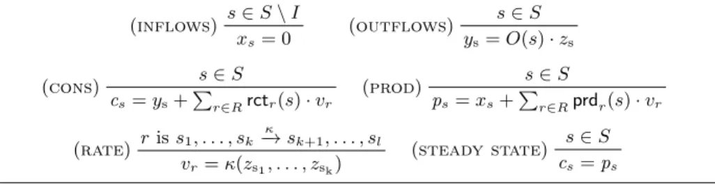
(inflows) s ∈ S \ I xs= 0 (outflows) s ∈ S ys= O(s) · zs (cons) s ∈ S cs= ys+Pr∈Rrctr(s) · vr (prod) s ∈ S ps= xs+Pr∈Rprdr(s) · vr (rate) r is s1, . . . , sk κ −→ sk+1, . . . , sl vr= κ(zs1, . . . , zsk) (steady state) s ∈ S cs= ps
Fig. 1: Steady state equations of a reaction network N = (S, R, I, O).
rate laws of chemical reactions. A chemical reaction r is a tuple of the form: s1, . . . , sk
κ
−→ sk+1, . . . , sl where 0 ≤ k ≤ l, s1, . . . , sl∈ S, and κ : Rk+→ R+ is a kinetic function. Any reaction has a tuple of reactants s1, . . . , sk and a tuple of products sk+1, . . . , sl. In order to account for the stoichiometry of a reaction, we write rctr(s) for number of occurrences of s in the tuple of reactants of r, and prdr(s) for number of occurrences of s in the tuple of products of r. A modifier of a reaction is a species s with rctr(s) = 1 = prdr(s). Whether a modifier behaves as an activator or as an inhibitor depends on the choice of the rate law κ. Definition 1. A reaction network over a species set S is a triple N = (S, R, I, O) where R is a finite set of chemical reactions over S, a set of inflow species I ⊆ S, and an outflow function O : S → R+.
A reaction network defines the evolution of a chemical solution in a context. Each inflow species s ∈ I specifies an inflow that adds s to the chemical solution, and is controlled by the context. An outflow species is an element s ∈ S with O(s) 6= 0; for any outflow species there is outflow into the context that consumes s from the chemical solution. The outflow kinetics for s follows the mass-action law with constant O(s). Note that any species may have an inflow and an outflow at the same time.
Under the assumption of deterministic network behavior, for any initial chem-ical solution a unique limit will be reached that is called a steady state. Since we do not fix any initial chemical solution, many steady states may exist for the same reaction network. The rates of all inflows and and outflows are also assumed to be constant in any steady state, as well as the rates of all reactions and the concentrations of all species of the network.
The steady state semantics of a reaction network is given by a system of arithmetic equations. These use the following variables taking values in R+. For any species s ∈ S, there is a variable zsthat denotes the concentration of s in a steady state, a variable xsthat denotes the rate of the inflow, which also called the influx, and a variable ys that stands for the rate of the outflow, which also called the outflux. For any reaction r ∈ R, variable vr stands for the rate of reaction r in a steady state.
The steady state equations are inferred from the network by the inference rules in Fig.1which are mainly standard. Each inference rule can be seen as an
Fig. 2: An enriched reaction with a partially known rate law ∼κ0. It has substrate S, in-hibitor I, accelerator A0, activator A, and one product P beside of the modifiers I, A, and A0.
I A’ A
P
S r
∼κ0
implication, whose condition is written above the line and whose conclusions is written below the line. Rules (inflow) states that the influx for any non-inflow species s 6∈ I is zero. Rule (outflow) requires for any species s ∈ S that its outflux is equal to O(s) · zs according to the mass-action law. The production rate ps of a species s is defined by rule (prod) and its consumption rate cs by rules (cons). Rule (rate) provides the rate of reaction r by applying its kinetic function to the concentrations of all its reactants. The (steady state) states that consumption and production rates are balanced for all species.
Definition 2. Any reaction network N with n inflow and m outflow species defines a exchange relation RN ⊆ Rn+× R
m
+, determined by the solutions of the steady state equations for N , when projected to the n-tuple of variables xs for the inflow species s of N and the m-tuple of variables ys0 for the outflow species s0 of N . The order of both tuples is given by the order ≺ on S.
3
Modeling Language
We now present a modeling language for reaction networks with partial kinetic information. As first parameter of our language, we assume a similarity relation ∼ on kinetic functions. Rather than specifying rate laws of chemical reactions by kinetic functions, we will describe them only up to similarity: a rate law belongs to ∼κ if it is similar to the kinetic function κ.
Enriched chemical reactions will be used to describe the chemical reactions of a reaction network. An example is given in Fig.2. The graph there represents an enriched chemical reaction r with substrate S, activator A, an accelerator A0, and inhibitor I and a product P . Please note that the same species may play different roles even in the same reaction, and several times. Both, activators and accelerators speed up a reaction. Activators are like enzymes. The difference is that all activators of a reaction must be present for its application, while the accelerators need not to be there.
For graphical representation, we use conventions similarly to Petri nets. Species are represented by rounded nodes s containing the name s of the species, and enriched reactions are graphically represented by boxed nodes r containing the name r of the reaction. More generally, enriched chemical reac-tions have different kinds of reactants, that are fixed by a finite set of roles Rol, which is the second parameter of our language. In our example, there will be substrates – that are consumed – and three kinds of modifiers: inhibitors, acti-vators, and accelerators, so we set Rol = {inh, subs, act, acc}. For our graphical syntax, we assign to each role an edge type, for edges pointing from the reactant
to the reaction. We will use for subs, for inh, for act , and for acc. The products of a reaction – beside of the above modifiers – will be linked by arrows pointing from the reaction to the product.
Reactant roles serve to order the arguments of the rate law of a enriched chemical reaction. Such a rate law is given by an enriched kinetic function:
κ0: (Rol × R+)k→ R+
We assume that any enriched kinetic function is well-behaved, in that any permu-tation of arguments with the same role does not change its value. When fixing the order of the arguments, any enriched kinetic function κ0 can be replaced by a standard kinetic function κ, for instance such that κ(zS, zI, zA0, zA) = κ0(subs: zS, inh: zI, act: zA0, acc: zA). An enriched chemical reaction can then be replaced by a chemical reaction, in which the kinetic function is replaced by a variable. With the same ordering as for obtaining κ from κ0, we obtain for the example from Fig.2:
S, I, A0, A−−→ P, I, A∼κ 0, A
Here, ∼κ stands for a fresh variable for a standard kinetic function that is sim-ilar to κ. A model in our language is a tuple (S, R, I, O) where R is a set of enriched reactions and I, O ⊆ S. Note that we do not require to specify rate constants for outflows. Graphically, inflow species in I and outflow species in O are indicated respectively by ingoing and outgoing arrows . An example model in graphical syntax is given in Fig. 3.
For any model in our language, we can generate a reaction network with vari-ables for kinetic functions that are subject to similarity constraints. Therefore, we can define the steady state equations of any model in the language as before, except that kinetic functions will be represented by variables, as well as rate constants of outflows. An example is worked out in the next section.
Besides the graphical syntax, our language supports an Xml syntax, which serves for writing the models, so that the graphs can be generated. We imple-mented tools for doing this in Xslt. These tools can also compute the steady state equations, and perform abstract interpretation.
4
Example: Regulation of Metabolism of B. subtilis
As an example, we model the leucine biosynthesis pathway of B. subtilis in our language. This is one of the complex regulation mechanisms of the metabolism of B. subtilis, for which informal models are given in the Subtiwiki [8]. The precise similarity relation of the model will be defined in Section5.
The resulting model in graphical syntax is given in Fig.3. For clearer visual-ization, nodes have different colors depending on the type of the species: in this paper we will use proteins P , metabolites M , and promoters or binding sites B . The variable zB stands for the activity of the promoter or binding site B, while zP and zMstand for the concentrations of P and M .
Leu CcpA CodY TnrA BSCodY PIlv−Leu BSTnrA r4 ∼exp r40 ∼ma r5 ∼exp r50 ∼ma r6 ∼exp r60 ∼ma r7 ∼exp r70 ∼ma r8 ∼ma r9 ∼ma r10 ∼ma
Fig. 3: Reaction network of the regulation of promoter PIlv-Leu in B. subtilis.
We consider an acceleration function with Acc(d) = 1 + d and an inhibition function with Inh(d) = 1/Acc(d). We define the enriched kinetic functions exp such that for all tuples t = (r1: d1, . . . , rk : dk) ∈ (Rol × R+)k:
exp(t) =Q
ri∈{subs,act}di · Q
rj=accAcc(dj) · Inh( P
rl=inhdl)
Note that the order of arguments with the same role is not important, so that function exp is well-behaved. When a reaction has the exp kinetics, then its inhibitors slow down the reaction but do not block it. Accelerators and activators both speed up the reaction. Furthermore, if one of the activators is missing then the reaction is blocked. One might want to generalize exp with parameters defining the strenght of respective accelerations and inhibitions. We do not do so, since these parameters are typically unknown, and since all such generalized expression kinetics will turn out to be similar. Generally, we are only interested in ∼exp, so similar definitions would to the job as well. The enriched mass-action kinetics is the special case ma(t) = exp(t) for all t ∈ ({subs} × R+)∗.
Leucine biosynthesis is realized by enzymes which are coded by the genes of the ilv-leu operon. This operon is under the regulation of the promoterPIlv−Leu. For simplicity, we group the whole reaction network leading to the leucine biosyn-thesis into reactionr8. The activation ofPIlv−Leuis done by reactionr5, under
regulation by TnrA, CcpA, and CodY. Proteins TnrA and CodY are influx species added by the context and degraded by reactionsr10 andr9respectively.
Protein CcpA is expressed by reaction r6 and degraded by reaction r60.
Tran-scription at the ilv-leu promoter is well known to be inhibited byCodYthrough a binding of this latter on the promoter [7,9,14,16,17]. To model this action of
CodY on the promoterPIlv−Leu, we introduce the reactionr4 which activates
the binding side BSCodY of CodY at the promoter, which in turn slows down
reaction r5 and thus reduces the promoter’s activity. The binding of CodY to
the promoter’s binding siteBSCodY can be prohibited whenCcpAis bound to
Flux balance equations: (Leu) vr8= yLeu (CcpA) vr6= vr60 (CodY) xCodY= vr9 (TnrA) xTnrA= vr10 (BSCodY) vr4= vr40 (PIlv−Leu) vr5= vr50 + vr8 (BSTnrA) vr7= vr70 Outfluxes:
yLeu= ma(8)(subs: zLeu) Reaction rates:
vr4 = exp
(1)(inh: z
CcpA, act: zCodY)
vr40 = ma(1)(subs: zBSCodY)
vr5= exp
(2)
(inh: zBSCodY, acc: zCcpA, inh: zLeu, inh: zBSTnrA)
vr50 = ma(2)(subs: zPIlv−Leu) vr6= exp (3) () vr60 = ma(3)(subs: zCcpA) vr7= exp (4) (act: zTnrA) vr70 = ma(4)(subs: zBSTnrA) vr8= ma (5)(subs: z PIlv−Leu) vr9= ma (6) (subs: zCodY) vr10= ma (7)(subs: z TnrA)
Fig. 4: Steady state equations for the PIlv-Leu network.
vr5= vr50+ yLeu
yLeu= ma(8)(subs: zLeu) vr4= exp
(1)(inh: z
CcpA, act: zCodY) vr4= ma
(1)
(zBSCodY)
vr5= exp
(2)
(inh: zBSCodY, acc: zCcpA,
inh: zLeu, inh: zBSTnrA)
vr50 = ma(2)(subs: zPIlv−Leu) vr6= exp (3) () vr6= ma (3) (subs: zCcpA) vr7= exp (4)(act: z TnrA) vr7= ma (4) (subs: zBSTnrA)
yLeu= ma(5)(subs: zPIlv−Leu) xCodY= ma(6)(subs: zCodY) xTnrA= ma(7)(subs: zTnrA)
Fig. 5: Simplified steady state equations for the PIlv-Leu network.
but it does not block it on average in a steady state. The promoter PIlv−Leu
is also down-regulated by Leu in terms of a T-box [1,4], which is captured by the negative control of the reaction r5 by Leu. Protein TnrA forms a further
inhibitor whose impact on the PIlv−Leupromoter is represented by the bind-ing side BSTnrA through the reaction r7. Protein CcpA is also independently
up-regulating the ilv-leu operon transcription, and thus activating reaction r5.
From the model, the steady state equations in Fig. 4 were inferred. These contain variables exp(i)for enriched kinetic functions similar to exp, and variables ma(i) for enriched kinetic functions similar to the mass-action law ma for any i. The equations can be simplified by replacing local variables by equal terms, yielding the equations in Fig.5.
In order to illustrate the qualitative reasoning methods that we will develop, we consider the overproduction problem ofLeufor thePIlv−Leunetwork. The question is which changes of the influxes may lead to an increase of the Leu
outflux? Informally, the problem can be solved as follows.Leuis produced only fromPIlv−Leu, which is solely produced by reactionr5, so the speed ofr5must
be increased. This can be done by either decreasing one of its three inhibitors
Leu,BSCodY, orBSTnrA, or by increasing its acceleratorCcpA. ButCcpAis not
connected to any inflow, so it cannot be increased by changing the influxes. And inhibitorLeucannot be decreased, when we want to increase its outflux. Hence,
eitherBSCodY orBSTnrAmust be decreased. This is possible only by decreasing
the influxes ofCodY orTnrA.
5
Similarity by Difference Abstraction
We now recall the similarity relation ∼ on kinetic functions from [5], which is obtained by abstracting from changes between real numbers.
We are interested in changes of the network raised for example by modifica-tion of inflows or outflows. A change of a concentramodifica-tion or a flow rate from one steady state to another is given by a pair of positive real numbers. We now want to abstract the space of all changes in R+× R+ into a finite set of difference relations. For this, we partition the set R+× R+into a finite collection of subsets ∆ ⊆ 2R+×R+, so that we can abstract any change in R
+×R+into a difference re-lation of ∆. In the examples that follow, we will use the partition ∆ = {<, >,=}. where the symbols represent “increase” < = {(x, y) ∈ R2+ | x < y}, “decrease” > = {(x, y) ∈ R2
+| x > y} and “no change” .
== {(x, x) | x ∈ R+}.
In general, we assume a relation R ⊆ Rp+, that may be either a kinetic function κ of arity p − 1 or the relation RN of a reaction network with p in- and outflows. We define the set of ∆-differences of the p-ary relation R as follows:
R∆= {(δ
1, . . . , δp) ∈ ∆p | ∀i. (di, d0i) ∈ δi, (d1, ..., dp) ∈ R, (d01, ..., d0p) ∈ R} So for instance, consider the exchange relation RN for some reaction network N . Its difference abstraction RN∆then expresses how the tuples in RN may change when moving from one steady state of N to another.
Definition 3. Two kinetic functions κ1, κ2 : (R+)p−1 → R+ are similar, written κ1∼ κ2, iff κ∆1 = κ∆2.
Example 1. Let mak(subs: d1, subs: d2) = k · d1· d2 be the mass action law with constant k. As usual, we identify binary functions with ternary relations. The differences abstraction mak∆is then equal for all choices of parameter k; it contains all triples of difference relations (δ1, δ2, δ3) ∈ ∆3given in the table on the right.
δ1 δ2 δ3 < < < < > <,=, >. < =. < > < <,=, >. > > > > =. > Example 2. We consider an enhanced Michaelis-Menten law with an additional activator: mmk1,k2(subs: d1, act: d2) = d2
k1· d1
k2+d1. Again, it can be shown that the abstraction (mmk1,k2)
∆
is independent of the choice of k1, k2∈ R+. Indeed, it is equal to mak∆for all parameters k, i.e.: mass-action and the enhanced Michaelis-Menten kinetics are similar with respect to ∆-abstraction, where ∆ = {<, >,=}.. Of course, there exist more precise difference sets ∆ for which the two families of kinetics can be distinguished.
It should be noticed that R∆ is always a finite relation, since ∆ is chosen to be finite. The relation R in contrast, may contain infinitely many tuples. As a consequence, infinitely much information may be abstracted away, in particular
the details about the parameters of kinetic functions. This is why the relations mak∆ and (mmk1,k2)
∆
in the above examples could be computed independently of the parameters. The information that is preserved, however, is still able to distinguish inhibitors and activators.
6
Abstract Interpretation to Difference Constraints
We next show how to interpret steady state equations abstractly as difference constraints, which will then be used for qualitative reasoning about reaction networks in our language in the next section.
The idea is to lift the difference abstraction .∆
from relations over R+ to relations over ∆ to the level of constraints defining such relations. For instance, the arithmetic equation xA = mak(zA, zB) can be abstracted to a difference constraint that defines the relation mak∆. We write this difference constraint as xA ∈ mak(zA, zB), since now the variables are interpreted by values of ∆ and mak is interpreted as the set valued function mak∆. It should be noticed that the relation mak∆ is finite and independent of the unknown parameter k, i.e., the unknown parameter has been abstracted away successfully.
Arithmetic constraints were used to define the steady state semantics of re-action networks. These are built from a totally ordered set of variables including those from the steady state equations. More formally, an arithmetic constraint is a conjunctive logic formula with existential quantifiers with the following ab-stract syntax:
φ ::= x=κ(i)(x1, . . . , xk) | x = x1+ x2| x1= x2| φ ∧ φ0 | ∃x.φ where i ∈ N, κ : Rk
+ → R+, and all x’es are variables. The expression κ(i) is a variable for a kinetic function that is similar to κ, i.e., an implicitly existentially quantified variable that is subject to the similarity constraint κ(i)∼ κ.
A solution of an arithmetic constraint φ with n variables can be identified with a tuple in Rn+ since we assumed a total order on the variables. The solution set sol (φ) of a formula φ satisfies sol (φ) ⊆ Rn+. For a reaction network N , the steady state equations are an arithmetic constraint φN such that sol (φN) = RN. A difference constraint is a conjunctive logic formula with existential quan-tifiers with the following abstract syntax, where x’es are variables and δ ∈ ∆:
difference relation t ::= x | δ
set of difference relations s ::= {t1, . . . , tn} | s + s0| s · s0 | Inh(s) | Acc(s) | κ(s1, . . . , sk) difference constraints ψ ::= t ∈ s | t=t0| ψ ∧ ψ0| ∃x.ψ
In contrast to before, all arithmetic operations now return sets of values in differ-ence constraints. Differdiffer-ence constraints are interpreted over ∆, so that variables x are assigned to elements of ∆ (rather than elements of R+). Arithmetic func-tions such as + are interpreted as set-valued funcfunc-tions on ∆ such as +∆, and similarly a kinetic function κ is interpreted as the set valued function κ∆.
vr5 ∈ vr50+ yLeu yLeu= zLeu
vr4 ∈ zCodY· Inh(zCcpA) vr4 = zBSCodY
vr5 ∈ zCcpA· Inh(zBSCodY + zLeu+ zBSTnrA)
vr50 = zPIlv−Leu vr6 = . = vr6 = zCcpA vr7 = zTnrA vr7 = zBSTnrA yLeu= zPIlv−Leu xCodY= zCodY xTnrA= zTnrA
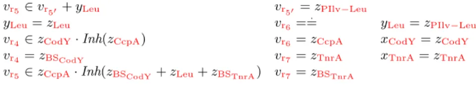
Fig. 6: Difference constraints for the PIlv-Leu network.
Since variables are totally ordered, a solution of a difference constraint can be identified with a tuple in ∆n, so that the solution set sol (ψ) of any difference constraint ψ satisfied sol (ψ) ⊆ ∆n.
We can now abstract from arithmetic constraints by interpreting them as difference constraints: Jx=κ (i)(x 1, . . . , xk)K = x ∈ κ(x1, . . . , xk) Jx = x1+ x2K = x ∈ x1+ x2 Jx1=x2K = (x1=x2) Jφ ∧ φ 0 K = JφK ∧ Jφ 0 K J∃x.φK = ∃x.JφK
An important point here is that the variables κ(i)for the partially known kinetic functions are replaced by well-known kinetic functions κ. For instance, we can abstract x = ma(i)(subs: x1) to x = x1, x = ma(i)(subs: x1, subs: x2) to x ∈ x1·x2, x = exp(i)() to x ==, and x = exp. (i)(subs: x1, inh: x2, inh: x3) to x ∈ x1· Inh(x2+ x3). This way, the simplified steady state equations for the PIlv−Leu network are abstracted to the difference constraints in Fig.6.
Theorem 1 (Soundness of Abstract Interpretation). sol (φ)∆⊆ sol (JφK). This theorem shows for any reaction network N that the solution set of the abstract interpretationJφNK is a correct over-approximation of the abstraction of the exchange relation RN∆:
Corollary 1. (RN) ∆
⊆ sol (JφNK).
Proof. This follows immediately from Theorem 1, since RN = sol (φN) by con-struction of φN.
7
Qualitative Reasoning with Difference Constraints
Since difference constraints have finite domains, we can compute all solutions of difference constraints by using finite domain constraint programming. Or else we can use constraint simplification for qualitative reasoning.
For instance, we can reconsider the question, which changes of the influxes of thePIlv−Leunetwork may increase the outflux of Leu. To find the answers, we can ask for the top-n solutions of the difference constraint yLeu = < in
(no1) Inh( . =) ⇒=. (no3) t · . = ⇒ t (ip) x + x ⇒ x (no2) Acc( . =) ⇒=. (no4) . = · t ⇒ t (si) t ∈ t0 ⇒ t = t0
(bv) ∃x. (x = t ∧ ψ) ⇒ ψ[t/x] (inh) t ∈ Inh(t + s) ⇒ t ∈ Inh(s)
Fig. 7: Simplification rules.
These solutions can be computed by the solver for difference constraints from [5], but extended with functions Inh and Acc in difference constraints.
There are only 5 solutions for this difference con-straint after projection to in- and outflux variables. These solutions are given to the right. The top-2 so-lutions with the fewest changes (1. and 2.) show that one can either decrease the influx of CodY or TnrA. The next three solutions show that one more change does not change the matter.
xCodYxTnrAyLeu
1. > =. < 2. =. > < 3. > > < 4. > < < 5. < > < Since thePIlv−Leunetwork is quite simple, one can obtain the same predictions based on constraint simplification. The simplification of the difference constraints in Fig.6 based on the rewrite rules in Fig.7 yields:
yLeu∈ Inh(xCodY+ xTnrA) .
When assuming yLeu = < in addition we can simplify the constraint further
to: < ∈ Inh(xCodY+ xTnrA) which is equivalent to xCodY = > ∨ xTnrA = >.
This can be satisfied by decreasing the influx of eitherCodYorTnrA. Thus, we obtain the same result as before.
In Fig. 7 we present simplification rules for difference constraints over the specific domain ∆ = {<, >,=}. Rule (bv) replaces equal by equal while elimi-. nating existentially bound variables (all variables zA and vri are implicitly
ex-istentially quantified). The simplification rules (noi) remove the nochange value .
=. The third rule (si) simplifies membership in singletons to equality. Rule (ip) expresses the idempotence of addition.
8
Conclusion
We have presented a formal modeling language for chemical reaction networks with partial kinetic information, and shown how to abstract away from the unknowns thanks abstract interpretation. We have illustrated that this allows us to reason qualitatively about such networks at the example of influx-change prediction. The same reasoning techniques are lifted to predict gene knockout strategies in follow-up work [2]. An important question for future work is how to develop finer abstractions for quantitative predictions.
References
1. Brinsmade, S.R., Kleijn, R.J., Sauer, U., Sonenshein, A.L.: Regulation of CodY Activity through Modulation of Intracellular Branched-Chain Amino Acid Pools. J. Bacteriol. 192(24), 6357–6368, 2010.
2. Coutte, F., Niehren, J., Dhali, D., John, M., Versari, C., Jacques, P.: Modeling Leucine’s Metabolic Pathway and Knockout Prediction Improving the Production of Surfactin, a Biosurfactant from Bacilus Subtilis. J. Biotechnology. To appear. 3. Forbus, K.D.: Qualitative reasoning. In: Tucker, A.B. (ed.) The Computer Science
and Engineering Handbook, pp. 715–733. CRC Press, 1997.
4. Grandoni, J.A., Zahler, S.A., Calvo, J.M.: Transcriptional regulation of the ilv-leu operon of Bacillus subtilis. Journal of bacteriology 174(10), 3212–3219, 1992. 5. John, M., Nebut, M., Niehren, J.: Knockout Prediction for Reaction Networks
with Partial Kinetic Information. In: 14th International Conference on Verification, Model Checking, and Abstract Interpretation. LNCS, 338-357, 2013.
6. Jungreuthmayer, C., Zanghellini, J.: Designing optimal cell factories: integer pro-gramming couples elementary mode analysis with regulation. BMC systems biology 6(1), 103, 2012.
7. Mäder, U., Hennig, S., Hecker, M., Homuth, G.: Transcriptional organization and posttranscriptional regulation of the Bacillus subtilis branched-chain amino acid biosynthesis genes. Journal of bacteriology 186(8), 2240–2252, 2004.
8. Mäder, U., Schmeisky, A.G., Flórez, L.A., Stülke, J.: Subtiwiki — a comprehensive community resource for the model organism bacillus subtilis. Nucleic acids research: 40(D1). 278-287, 2012.
9. Molle, V., Nakaura, Y., Shivers, R.P., Yamaguchi, H., Losick, R., Fujita, Y., So-nenshein, A.L.: Additional targets of the Bacillus subtilis global regulator CodY identified by chromatin immunoprecipitation and genome-wide transcript analysis. Journal of bacteriology 185(6), 1911–1922, Mar 2003.
10. Orth, J.D., Thiele, I., Palsson, B.O.: What is flux balance analysis? Nature biotech-nology 28(3), 245–248, 2010.
11. Otero, J.M., Nielsen, J.: Industrial systems biology. Industrial Biotechnology: Sus-tainable Growth and Economic Success, 2010.
12. Papin, J.A., Stelling, J., Price, N.D., Klamt, S., Schuster, S., Palsson, B.O.: Com-parison of network-based pathway analysis methods. Trends in biotechnology 22(8), 400–405, 2004.
13. Price, N.D., Reed, J.L., Palsson, B.O.: Genome-scale models of microbial cells: evaluating the consequences of constraints. Nature reviews. Microbiology 2(11), 886–897, 2004.
14. Shivers, R.P., Sonenshein, A.L.: Activation of the Bacillus subtilis global regulator CodY by direct interaction with branched-chain amino acids. Molecular microbi-ology 53(2), 599–611, 2004.
15. Sohn, S.B., Kim, T.Y., Park, J.M., Lee, S.Y.: In silico genome-scale metabolic analysis of Pseudomonas putida kt2440 for polyhydroxyalkanoate synthesis, degra-dation of aromatics and anaerobic survival. Biotechnol. J. 5(7), 739–750. 2010. 16. Tojo, S., Satomura, T., Morisaki, K., Deutscher, J., Hirooka, K., Fujita, Y.:
Elab-orate transcription regulation of the Bacillus subtilis ilv-leu operon involved in the biosynthesis of branched-chain amino acids through global regulators of CcpA, CodY and TnrA. Molecular Microbiology 56(6), 1560–1573, 2005.
17. Villapakkam, A.C., Handke, L.D., Belitsky, B.R., Levdikov, V.M., Wilkinson, A.J., Sonenshein, A.L.: Genetic and Biochemical Analysis of the Interaction of B. subtilis CodY with Branched-Chain Amino Acids. J. Bacteriol. 191(22), 6865–6876, 2009.