Integrated Population Models and Habitat Metrics for Wildlife Management

(1)

Integrated Population Models and Habitat Metrics

for Wildlife Management

Thèse

James Nowak

Doctorat en sciences forestières

Philosophiae Doctor (Ph.D.)

Québec, Canada

© James Nowak, 2015

(2)

(3)

III

RÉSUMÉ

La gestion des espèces est entièrement dépendante de notre capacité à évaluer les décisions de gestion et de les corriger si nécessaire. Dans un monde idéal les gestionnaires auraient une connaissance extensive et mécanistique des systèmes qu’ils gèrent et ces connaissances seraient mises à jour de façon continue. Dans la réalité, les gestionnaires doivent gérer les populations et développer des objectifs de populations en dépit de leur connaissance imparfaites et des manques de données chronique. L’émergence de nouveaux outils

statistiques ouvrent toutefois la porte à de nouvelles possibilités ce qui permet une gestion plus proactive de la faune. Dans le Chapitre 1, j’ai évalué l’efficacité de modèles intégrés de populations (MIP) à combler des lacunes dans notre connaissance en présence de données limitées et de modèles de populations mal spécifiés. J’ai démontré que les MIP peuvent maintenir une précision élevée et présenter un biais faible, et ce dans une large gamme de conditions. Dans le chapitre 2, j’ai développé une approche de MIP qui inclut des effets aléatoires entre les différentes populations. J’ai constaté que les effets aléatoires permettent améliorer considérablement les performances des algorithmes d'optimisation, produisent des estimations raisonnables et permettent même d'estimer les paramètres pour les populations avec des données très limitées. J’ai par la suite appliqué le modèle à 51 unités de gestion du Wapiti en Idaho, USA afin de démonter son application. La viabilité des populations à long terme est généralement réalisé à grâce à des manipulations d’habitat qui sont identifiées grâces à des méthodes de sélection des ressources. Les méthodes basées sur la sélection des ressources assume cependant que l’utilisation disproportionnée d’une partie du paysage reflète la volonté d’un individu de remplir une partie de son cycle biologique. Toutefois, dans le troisième chapitre j’ai démontré que des simples mesures d’habitat sont à mieux de décrire la variation dans la survie des Wapitis. Selon, mes résultats, la variation individuelle dans la sélection des habitats était le modèle qui expliquait le mieux la corrélation entre les habitats et le succès reproducteur et que les coefficients de sélection des ressources n’étaient pas corrélés à la survie.

(4)

(5)

V

ABSTRACT

Successful management of harvested species critically depends on an ability to predict the consequences of corrective actions. Ideally, managers would have comprehensive, quantitative and continuous knowledge of a managed system upon which to base decisions. In reality, wildlife managers rarely have comprehensive system knowledge. Despite imperfect knowledge and data deficiencies, a desire exists to manipulate populations and achieve objectives. To this end, manipulation of harvest regimes and the habitat upon which species rely have become staples of wildlife management. Contemporary statistical tools have potential to enhance both the estimation of population size and vital rates while making possible more proactive management. In chapter 1 we evaluate the efficacy of integrated population models (IPM) to fill knowledge voids under conditions of limited data and model misspecification. We show that IPMs maintain high accuracy and low bias over a wide range of realistic conditions. In recognition of the fact that many monitoring programs have focal data collection areas we then fit a novel form of the IPM that employs random effects to effectively share information through space and time. We find that random effects dramatically improve performance of optimization algorithms, produce reasonable estimates and make it possible to estimate parameters for populations with very limited data. We applied these random effect models to 51 elk management units in Idaho, USA to demonstrate the abilities of the models and information gains. Many of the estimates are the first of their kind. Short-term forecasting is the focus of population models, but managers assess viability on longer time horizons through habitat. Modern approaches to understanding large ungulate habitat requirements largely depend on resource selection. An implicit assumption of the resource selection approach is that disproportionate use of the landscape directly reflects an individual’s desire to meet life history goals. However, we show that simple metrics of habitat encountered better describe variations in elk survival. Comparing population level variation through time to individual variation we found that individual variation in habitat used was the most supported model relating habitat to a fitness component. Further, resource selection coefficients did not correlate with survival.

(6)

(7)

VII

LIST OF TABLES

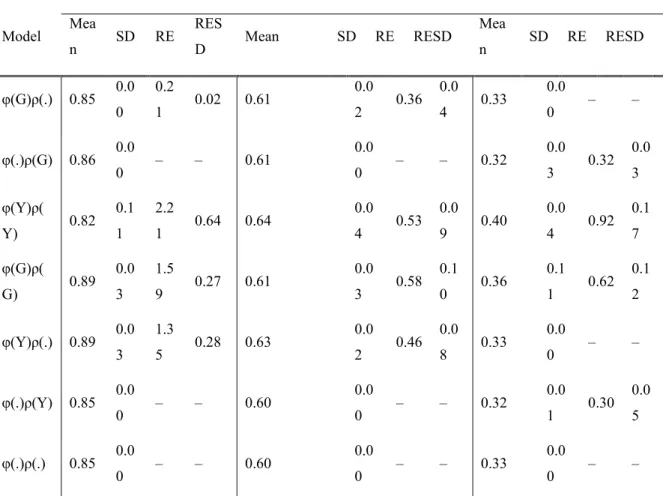
Table 2-1 Model comparison results of integrated population models applied to elk populations in Idaho (1985-2011). Where G represents a spatial random effect delineated by game management unit and Y indicates a random effect of year on adult elk survival (φ) and recruitment of young (ρ) respectively and a period indicates the parameter was held constant. ... 54 Table 2-2 Parameter estimates obtained from the seven fitted models for adult female survival (φf_{), adult male survival (φ}m_{), recruitment (ρ) and random effects (RE). When} parameters were assumed constant demographic rates represent the mean and standard deviation of the posterior distribution. When random effects were considered the estimate reflects the population level (i.e. global) mean and standard deviation of the posterior distribution. Columns with heading RE depict the standard deviation of the hierarchically centered random effect with the uncertainty about that estimate following in the RESD column. The -- denotes the exclusion of a parameter from a given model. ... 55 Table 3-1 Top five elk survival models for each combination of data considered. The top sets of five models related resource selection coefficients to survival while the bottom sets of five considered habitat encountered. Similarly, the left side of the table represents models focusing on individual variation and the right side considers time varying population level effects. Each row of the table depicts a unique model. Models are defined by 1/0 indicating the presence/absence of a variable. For example, a model coded as 00110 would include the effects of fire year and road density. The furthest right column contains posterior model probabilities. Note that the intercept always considered 5 age classes and animal sex was always included as an indicator variable. ... 86

(12)

(13)

XIII

LIST OF FIGURES

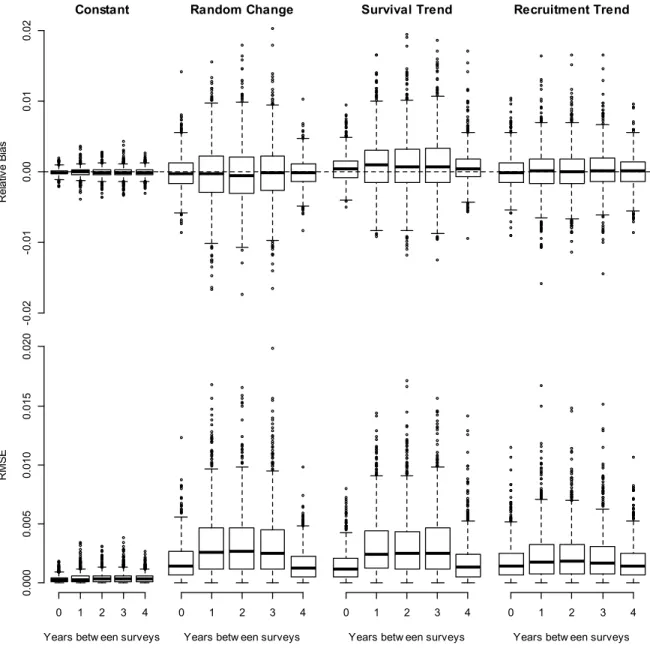
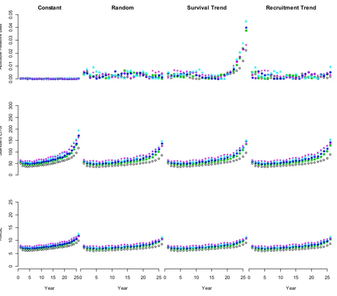
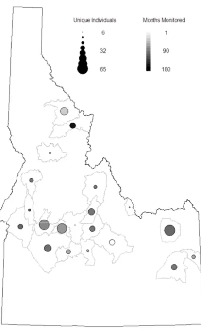
Figure 1-1 Simulation study survival estimates. Vertically boxplots are arranged by simulation scenario (constant, random temporal variability, survival trend and recruitment trend). Within each scenario five levels of missing data are compared. On the y-axis we present bias, precision (SE) and accuracy (RMSE) of estimates. ... 25 Figure 1-2 Simulation study recruitment estimates. Vertically boxplots are arranged by simulation scenario (constant, random temporal variability, survival trend and recruitment trend). Within each scenario, five levels of missing data are compared. On the y-axis we present bias, precision (SE) and accuracy (RMSE) of estimates. ... 26 Figure 1-3 Boxplots of relative bias and root mean squared error of geometric mean growth rates from 1,000 simulations. The number of years between aerial surveys is depicted on the x-axis. Simulation scenarios, from left to right, include correct/constant model specification, extra random variation, linear trend in adult survival and a linear trend in recruitment. ... 27 Figure 1-4 Plots display mean absolute relative bias, standard error and root mean squared error (RMSE) of adult female population size estimates over the 26 step time-series. Black open circles represent mean estimates without missing data. The remaining color shape combinations represent the number of years of missing data where filled green squares, filled dark blue circles, filled light blue triangles and filled pink diamonds represent one through four years of missing data between surveys. ... 28 Figure 1-5 Plots display mean absolute relative bias, standard error and root mean squared error (RMSE) of young of year population size estimates over the 26 step time-series. Black open circles represent mean estimates without missing data. The remaining color shape combinations represent the number of years of missing data where filled green squares, filled dark blue circles, filled light blue triangles and filled pink diamonds represent one through four years of missing data between surveys. ... 29 Figure 1-6 Comparison of adult survival estimates. Dashed gray lines represent posterior density estimates derived from an inverse matrix model using only stage structured aerial survey data of elk in Idaho, USA. Solid black lines depict posterior densities from an IPM considering aerial survey and telemetry data. Dotted black lines characterize estimates obtained from analysis of telemetry data in isolation of aerial survey data. ... 30 Figure 1-7 Posterior density plots of recruitment estimates. Dashed gray lines represent posterior density estimates derived from inverse-matrix model using only stage structured aerial survey data. Solid black lines show recruitment estimates derived from IPM with aerial survey and telemetry data. Tick marks at the bottom of each plot portray age ratio estimates obtained during aerial surveys. Dotted tick marks depict estimates from independent data collected during composition surveys. ... 31 Figure 2-1 Aerial Survey data collection schematic showing the year of data collection on the bottom, spatial unit of collection on the left, the number of aerial surveys per year on

(14)

XIV

top, and the number of full aerial surveys per unit on the right. Full aerial surveys and herd composition flights are represented by filled black dots and filled gray dots respectively. 56

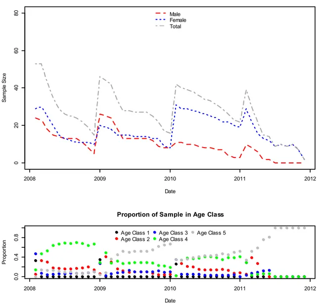
Figure 2-2 Spatial extent of the study area where shaded units indicate inclusion. Gray scale values also indicate the number of full aerial surveys conducted since 1985. ... 57 Figure 2-3 Telemetry data used in the study. The size of the dots represents the number of unique individuals monitored in the GMU while the grey scale of the dot is used to show the number of months the GMU had a sample size ... 58 Figure 2-4 Mean estimate of adult survival (Left: Female, Right: Male) by game management unit. Estimates taken from the most supported model. Darker colors correspond to lower survival, but note that while the scales are different the relative difference in survival is similar. ... 59 Figure 2-5 Geometric mean growth rate derived from annual population estimates from 1985-2011 presented on the left. The map on the right shows the probability that the value is > 1. Units in white were estimated to be growing with a probability of 1. Units in black represent those units with little to no chance of have experienced growth since 1985. ... 60 Figure 2-6 Comparison of demographic rate estimates from GMU 43 as suggested by the most supported model (φ(G)ρ(.)) and a model considering GMU 43 in isolation with constant demographic rates. Black lines show posterior densities estimated by the random effects model while the gray lines depict the single unit analysis. This analysis is included to illustrate the data sharing qualities of a random effects parameterization. ... 61 Figure 3-1 A plot of the changing sample size through time and the proportion of the sample comprised of 5 age classes used to model survival. The top panel displays the number of collared male elk with a dashed red line, while the number of collared female elk is represented with a dotted blue line. Atop both of these lines is the total sample size or the total number of collared elk in each month. Resource selection models were fit with data from both sexes (dashed and dotted gray line). The bottom panel shows which age classes comprise the sample. The five age classes were delineated such that animals ≤ 1 year of age were placed in age class 1, animals > 1 and ≤ 2 years of age in age class 2 and so on until age class five, which represents animals older than 4 years of age. To create the plot we started the animal at the estimated age at capture and subsequently aged the animal each year. ... 87 Figure 3-2 Plots of monthly habitat selection by elk in Idaho, USA. Colored dots show mean estimates while vertical bars depict 95% confidence intervals. Dots are coded such that the color signifies the year of the estimate where black, red, green and blue represent 2008, 2009, 2010 and 2011 respectively. A dashed line is included in each plot to mark 0, the point at which environmental variables are used equal to their availability. ... 88

(15)

XV

LIST of APPENDICES

Appendix 1-1 Posterior density plots of estimated elk recruitment rates for 51 administrative units in Idaho, USA (1985 – 2011). Estimates were computed using inverse methods that considered only age-structured abundance estimates collected at irregular intervals. ... 32

Appendix 1-2 Posterior density plots of estimated adult elk survival rates for 51 administrative units in Idaho, USA (1985-2011). Estimates were computed using inverse methods that considered only age-structured abundance estimates collected at irregular intervals. ... 33

Appendix 3-1 Age and sex specific elk survival estimates. Ages reference age-at-capture. An indicator variable represented whether an animal was a female or not. Models used a means parameterization for age and an effects parameterization for the effect of sex. Models that produced the estimates shown here did not include any habitat covariates. ... 89

(16)

(17)

1

General Introduction

Successful management of harvested species critically depends on an ability to predict the consequences of corrective actions. Ideally, managers would have comprehensive, quantitative and continuous knowledge of a managed system upon which to base decisions that seek to meet clearly defined, publicly agreed upon objectives (Lindblom 1959; Bailey 1982). In reality, wildlife managers rarely have comprehensive system knowledge. Limited data and imperfect system knowledge result from several factors. First, wildlife populations are notoriously difficult to count. Second, monitoring programs cannot produce ideal data sets because of constraints imposed by logistical and budgetary realities. Third, wildlife population dynamics are complex, variable and subject to multiple stressors that have complex interacting effects. Despite imperfect knowledge and data deficiencies, a desire, and—in some cases—a legal obligation exists to manipulate populations and achieve objectives. To this end, manipulation of harvest regimes and the habitat upon which species rely have become staples of wildlife management.

Proactive species management depends on an ability to identify a preferred course of action before implementation. Consequently, proactive management suggests defining a model with strong predictive abilities. The objective of the model then is to exemplify the principle of parsimony while making accurate predictions and accounting for uncertainty in biological and observational processes (Nichols & Williams 2006). A desirable secondary objective of the model might include identifying causes of increase or decline, but this goal typically outstrips the data available to many species monitoring programs. Historically, many management programs relied on trend detection to incite action. However, trend detection relegates management to a reactionary posture while proactive management strategies aim to maintain species near management goals in lieu of continually responding to large deviations from objectives.

Big game management in the Rocky Mountain West, USA, has become a contentious topic steeped in litigation and public opinion. Much of the debate surrounds the re-introduction of the gray wolf (Canis lupus) and the consequences for socially and economically

(18)

2

important ungulate species, in particular elk (Cervus elaphus). Nowhere is this more apparent than in Idaho. Approximately 78,000-84,000 hunters enjoy elk hunting in Idaho each year. Elk hunters generate approximately 150 million dollars in annual revenue, which represents the largest single financial contribution from the exploitation of any one species (Cooper et al. 2002). Managers strive to meet management objectives and maintain a harvestable surplus in the face of uncertainty, but the roles of multiple interacting factors in regulating or limiting elk populations remain undefined despite a large body of research.

Having demonstrated a desire to pursue proactive management, chapters 1 and 2 address the feasibility of filling knowledge voids using integrated population models (IPM). IPM’s provide a particularly powerful approach to population modeling by piecing together disparate sources of data (Besbeas et al. 2002; White & Lubow 2002; Brooks, King & Morgan 2004; Conn et al. 2008; Schaub & Abadi 2011). Typical sources of data may include aerial counts, radio-tagging encounter histories, productivity indices, harvest surveys and environmental data. By combining all or several of these sources of data into one analysis, it is possible to obtain more robust (and self-consistent) parameter estimates that fully reflect the information available and the true state of the system (Besbeas et al. 2002). A synthetic approach is desirable because analyzing demographic rates in isolation ignores dependencies among rates that produce observed outcomes (Baillie 1991). Other advantages of integrated approaches are the ability to estimate latent or unobserved quantities (Abadi et al. 2010b; Schaub et al. 2010), increased precision of parameter estimates and so-called honest accounting of error (Besbeas et al. 2002; Clark & Bjørnstad 2004). Further IPM’s provide a biologically, if not legally, defensible basis for management actions and more efficient allocation of scarce resources. The framework’s flexibility accommodates the many complexities inherent to population monitoring and allows for mechanistic linkages between population size and demographic processes. Last, the framework has withstood public scrutiny and proven effective within the context of collaborative structured decision-making (Freddy et al. 2004; Thompson 2014).

Short-term forecasting is the focus of population models, but managers assess viability on longer time horizons through habitat. Modern approaches to understanding large ungulate

(19)

3 habitat requirements largely depend on resource selection functions (RSF, (Manly, McDonald & Thomas 1993). An implicit assumption of the RSF approach is that disproportionate use of the landscape directly reflects an individual’s desire to meet life history goals. However, recent evidence suggests that animals may not employ the “best” strategy that results in maximized fitness (Arlt & Pärt 2007; DeCesare et al. 2013). Several ecological hypotheses suggest the existence of non-ideal habitat selection strategies. Should habitat selection models not remain faithful to individual performance their application to species management could result in misallocation of resources and failure to meet objectives. The third chapter addresses this idea by evaluating estimates of resource selection with survival models.

Harvest and habitat represent two foundational components of species management. Through the combination of modern statistical techniques and ecological knowledge, the following document enhances our understanding of current elk population models and dynamics. The last chapter then tests a critical assumption of habitat models, which illuminates their applicability to long-term assessments of population viability.

(20)

(21)

5

Chapter 1. Evaluating Bias, Accuracy and

Precision when Fitting Population Models to

Limited Data

Résumé

Les gestionnaires de la faune doivent définir des objectifs de populations et travailler à la gestion de ces populations, et ce indépendamment de la disponibilité des données. La gestion des espèces est une tâche assujettie à des contraintes de temps et devrait donc bénéficier du développement d’analyses quantitatives et de modèles. Les cadres de modélisation formelles fournissent un moyen de synthétiser les données tout en tenant compte des nuisances caractéristiques des données, ce qui augmente l'accessibilité des données et l'efficacité de la gestion tout en décrivant l'état d'un système et l'état des connaissances du système. Une approche particulièrement puissante pour la modélisation des populations qui consiste à assembler plusieurs sources de données disparates est d’utiliser un modèle de population intégré (PMI). Les données disponibles pour la modélisation des populations sont toutefois généralement perçues comme étant top limité pour les PMI. De plus les données disponibles peuvent avoir un couvrir des espaces ou des séquences de temps disparate. Pour surmonter ces problèmes, nous avons développé une approche nouvelle qui permet le partage d’information à travers le temps et l’espace grâce à l’utilisation d’effets aléatoires dans le modèle. Nous avons utilisé la sélection de modèles afin de comparer différents scénarios qui pourraient expliquer variation des taux démographiques dans le temps ou dans l'espace. Le modèle qui a tenu le recrutement constant et la survie des adultes constante temporellement, mais variable spatialement a reçu le plus de support. À l’échelle de l’état, les modèles qui ont reçu le plus de support suggèrent que la survie des a femelles adultes a oscillé autour de 0.85 (SD = 3.7E-4), la survie des mâles a oscillé autour de 0.61 (SD = 2.0E-3) tandis que le recrutement a été presque constant à 0.33 (SD = 1.3E-3). Compte tenu de nos résultats, la survie des adultes a plus de chances d’affecter la dynamique des populations de Wapiti en Idaho que les variations dans le recrutement. Les variations dans la survie des adultes sont probablement

(22)

6

attribuables aux fluctuations dans la récolte. L’utilisation des PMI s'appuyant sur l’utilisation d’effets aléatoires nous a permis de combiner plusieurs sources de données et nous a permis d’augmenter la précision des estimations, tout en nous permettant de traiter les données manquantes et les nombreuses particularités de notre jeu de données.

(23)

7

Abstract

Estimation of demographic rates and population size is central to the study of ecology and species management. Combining such estimates with matrix projection models allows researchers to simulate population dynamics. However, these problems are better framed as matters of parameters estimation. Inverse matrix models allow estimation of demographics rates and abundance from a time-series of observations. Integrated population models build upon inverse methods to facilitate the use of multiple sources of data while fitting model parameters. Interest in applying these methods to real life scenarios motivated this study in which we used simulation to evaluate the performance of inverse methods under conditions of missing data and model misspecification. To emulate low frequency data collection we simulated data according to five frequencies of data collection, zero to four years between observations. In addition to missing data, we also simulated three scenarios of model misspecification using linear trends and stochastic variation. We then fit inverse matrix models and integrated population models to aerial survey and telemetry data on elk in Idaho, USA. Results from simulations indicated adequate accuracy, precision and bias from inverse matrix methods regardless of data collection frequency or model misspecification. Furthermore, model estimates were most sensitive to misspecification involving adult female survival. Fitting inverse and integrated population models to elk data resulted in similar estimates of demographic rates and abundance. These estimates are the first of their kind for a majority of the administrative units considered. Our results suggest that fitting population models to limited noisy data is not only possible, but under many circumstances will increase the amount and quality of information available for species management.

(24)

8

Introduction

Estimating demographic rates and population size is central to the study of ecology and species management. Population monitoring seeks to quantify demographic rates, changes in those rates and the resulting population size (Williams, Nichols & Conroy 2002). This information is critical for effective and predictable management of populations. However, logistical and financial constraints typically prohibit the collection of exhaustive data sets. Noisy, incomplete and disparate data are the rule when it comes to population monitoring (Clark & Bjørnstad 2004). Despite data deficiencies, a desire exists to predict future populations, establish current population status and defend management decisions (Freddy

et al. 2004). To this end, matrix population models have gained immense popularity for

their relative simplicity, flexibility and their ability to simultaneously handle noisy, incomplete data while addressing key management questions (Caswell 2006).

The use of a matrix model typically proceeds by first estimating mean demographic rates by age, sex or other delineations (Lefkovitch 1965). Future population dynamics are then projected by repeatedly multiplying a population vector by the demographic matrix under the assumption that demographic rates are known without error. The ensuing time-series of population abundances can then be compared to observed abundances (Caswell 2006). Such a simulation-based approach to monitoring is feasible when data describing demographic rates are readily available. However, it is generally only abundances that are commonly estimated by many monitoring programs and simulation-based approaches relegate these hard-earned demographic estimates to the model validation stage. While seemingly attractive, the use of abundance data to validate simulations encourages the modeler to arbitrarily manipulate demographic rates until population projections and abundance data “agree”. As noted by White and Lubow (2002), this problem is better posed as a matter of statistical parameter optimization and methods exist to estimate the parameters of population models from data.

One class of model that uses a time-series of abundance estimates to estimate demographic rates are so-called inverse matrix models (Gross, Craig & Hutchison 2002; Buckland et al.

(25)

9 2004; Caswell 2006; Wielgus et al. 2008). The term inverse comes from the fact that the models estimate the demographic rates from count data whereas simulation based approaches use demographic rates to produce abundance estimates. Despite differences in how they use data both methods rely on a common demographic projection matrix to specify population transitions through time. The projection matrix describes the biological process of interest. For species where age or stage classification is possible, fitting a model within the inverse framework affords a non-invasive means of estimating demographic rates (Wielgus et al. 2008).

Recently developed integrated population models (IPM) offer an opportunity to bolster inverse methods by estimating demographic rates and population size from multiple sources of data (Besbeas et al. 2002; Brooks, King & Morgan 2004). Thus, an IPM is nothing more than an inverse matrix model that incorporates auxiliary data on demographic parameters. (Schaub & Abadi 2011) defined integrated population models as any model that “jointly analyses data on population size and data on demographic parameters”. Thus, the primary difference between inverse methods and an IPM is the inclusion of supplementary data on the demographic rates of interest. Typical sources of data may include aerial counts, radio-tagging encounter histories, productivity indices, harvest surveys and environmental data. The flexible and synthetic nature of IPM’s makes them an attractive tool for species management and conservation (e.g Schaub et al. 2007; King et al. 2008; Johnson et al. 2010).

Wildlife monitoring programs often cover large spatial extents comprised of many smaller administrative units with heterogeneity in the quality and quantity of data available. Heterogeneity in data availability challenges our ability to apply a single model to all administrative units. However, progressing from inverse to IPM methods does not necessitate change in the demographic projection matrix. At the complex end of the spectrum, data-rich populations might exploit a full IPM with multiple types of data while data-poor populations will necessarily require simpler inverse methods relying solely on abundance estimates. The key advantage of a consistent approach is that the same demographic projection matrix can be used to model population transitions in any

(26)

10

population across a wide range of data quantities and qualities. Consistency in the modeling approach offers a unifying framework for the analysis of monitoring data while making possible comparative studies, objective optimization of management alternatives and iterative learning from past action all while providing critical information to decision makers.

In this paper, we use simulation to quantify the accuracy, precision and bias of inverse matrix models and then fit inverse models to field data for comparison with an IPM and demographic rate estimates considered in isolation. Having identified at the outset that real data sets are typically far from ideal, we are interested in quantifying model accuracy, precision and bias in the face of missing data and model misspecification. We imagine that in practice supplementary data will only be available for a subset of populations. Models describing data-poor units will unfortunately be bottlenecks for model reality and performance. Past assessments of IPM’s demonstrated the capabilities of the methods under data-rich circumstances (Abadi et al. 2010a). Here simulations focus on a worst-case scenario where no supplementary data exist (i.e. an inverse model). The first problem addressed by simulation involves missing values in survey data. Missing values are imagined to be the result of only quantifying abundance every 1 to 5 years. We believe an evaluation with missing data to be critical if these methods are to have utility in monitoring programs. Second, we evaluate model performance under three scenarios of misspecification plus one scenario using a correctly specified model. For clarity, the term misspecification is used to describe a situation where data were simulated using a model that did not match the way in which the data were subsequently analyzed.

Specifically, we first consider the effects of misspecification by simulating demographic rates that vary randomly in time, but are modeled as constant parameters. Second, we evaluate linear temporal trends that are present in the data, but not modeled in the survival or recruitment processes. Scenarios of misspecification are important in a management context because limited data will typically dictate the use of reduced parameter models and so misspecification is likely to occur. Quantifying accuracy, precision and bias when models are knowingly misspecified helps to quantify their value when data are limited.

(27)

11 Finally, we conclude the analyses by estimating demographic parameters for 51 populations of elk (Cervus elaphus) with inverse methods, an IPM and estimate adult survival in isolation. Through these steps, we highlight information gains, the necessary quantification of uncertainty and time-series complexity. Finally, we discuss accessibility of the models and inferential considerations.

Methods

To evaluate the feasibility of the inverse methods for sparse data we simulated time-series data for 26 years and then fit models to the simulated time-series using a state-space formulation of an inverse matrix model. Parameter values used in the simulations were chosen to emulate the characteristics of elk demographic rates in Idaho, USA. We then fit models to aerial survey data of 51 elk populations using a state-space inverse matrix model. Following initial model fit, supplementary telemetry data were added to the model structure resulting in an IPM. Finally, telemetry data were used to separately estimate survival for comparison. Fitting multiple models to field data facilitated graphical presentation of comparisons among inverse, IPM and demographic data estimates.

Field Data

We used data from the research and routine monitoring activities of Idaho Department of Fish and Game (IDFG). We considered data from 51 game management units (GMU) in Idaho. Data span the 26-year period from 1985 to 2011. GMUs were included in the study if they met two criteria. First, we included only those units where the number of aerial surveys conducted between 1985 and 2011 was greater than 1. Second, we considered only GMUs where aerial surveys were designed to produce estimates representative of population size, which eliminated GMUs strictly monitored for trends in the north of the state. Consequently, aerial survey data used here were assumed representative of population size.

(28)

12

Aerial surveys occurred at irregular intervals leading to many missing values and temporal patchiness in data quantities. Surveys occurred in January, February or March. Surveys were generally not flown in the same year for multiple adjacent GMU’s, which created spatial patchiness in the sampling protocol and precluded spatial aggregation of units, but created an opportunity for units to inform neighboring non-sampled units. However, some units were flown in aggregate with other GMU’s during data collection, which restricted our ability to maintain a common spatial unit of organization. Data collected during full aerial surveys included estimates of female, male and calf elk counts. Periodic composition surveys, which are less onerous than full aerial surveys, were used to estimate age ratios. Raw counts from full surveys were adjusted for visibility bias using the software Aerial Survey 6 (Unsworth et al. 1999a). The details of the software and the visibility correction are described in Samuel et al. (1987). We used the estimated mean and variance of adjusted count data as observations because raw count data were not available for this study.

Data on elk survival consisted of summaries of 641 telemetry collar deployments, including date of deployment, date of recovery of sensor, sex of the animal and field based age-class estimates. Collars were a mixture of GPS and VHF technologies and manufacturers. Collar deployments spanned a wide geographic range with deployments originating in 21 unique GMU’s. Adult elk were captured by helicopter darting or net-gunning, drive nets or corral traps during winter of each year. Animals were fitted with telemetry collars equipped with mortality sensors. IDFG personnel typically monitored the animal’s fate by fixed wing aircraft on, at least, a monthly basis.

Demographic Projection Matrix (Process Model)

We maintained consistency among all populations by using the same demographic projection matrix (i.e. biological process) to fit simulated and field data regardless of the method applied (e.g. IPM, inverse). The demographic projection matrix we used followed a discrete time, two-stage, single sex structure where individual females reproduce for the first time in their second year of life. We set the model anniversary to occur in February to approximate when IDFG conducts aerial counts of elk. We fit models assuming that

(29)

13 demographic rates are constant and the population is closed to immigration and emigration. The model also assumed that males and females were produced in equal proportions. The most general process equations fit to data were as follows:

~ ∗

~ ∗ 0.5 , .

Where the number of young ( ) at annual time step 2 to t was assumed to be a Poisson distributed variable with mean equal to the product of the number of adult females in the current time step and a recruitment term ( ). The annual number of adult females ( ) was considered the outcome of a binomial trial where the sum of half the number of young in the previous time step and the number of adults in the previous time step experience survival at a rate equal to for time steps 2:t. We assume, therefore, that count data can differentiate young from adults and further that age classification is correct.

The recruitment term ( ) describes the number of young of the year that are born and survive to be counted per adult female. Recruitment was restricted to the range (0, 1) because twinning is rare in elk (Toweill, Thomas & Metz 2002). In wildlife literature this term is commonly called an age ratio. Age ratios can be difficult to interpret because the numerator and denominator both vary according to separate, but likely correlated, biological processes (Caughley 1974). Nevertheless, we suppose that for many populations age ratios will be available whereas specific information about pregnancy rates, fecundity and survival of young may not. Additionally, there is some support that age ratios may be a reliable index of recruitment in elk populations (Harris, Kauffman & Mills 2008).

Simulations

To evaluate inverse matrix model performance we first simulated population time-series’ using the above demographic projection matrix and distributions. The initial population

(30)

14

size of adults and young were 6000 and 2000 respectively for all simulations. These values reflect the estimated abundances in GMU 10 in 1985 and do not conform to a stable-stage distribution (SSD) assumption. Thus, the population simulations begin with transitory dynamics. We simulated 1,000 population time-series for each of four scenarios at five levels of missing data for a total of 20,000 simulations. Model parameters were stochastically drawn for each iteration. We added observation uncertainty to simulations by assuming that population sizes generated by the process models above were observed according to a Poisson process with mean equal to and for adults and young respectively. Our choice of distribution to describe observation uncertainty was one of convenience, but it also ensured that variance increased as the mean increased. All simulations projected population dynamics for 26 years, the length of data available to Idaho Department of Fish and Game. Our four scenarios were constant adult survival and recruitment of young (i.e. correctly specified), random variation in adult survival and recruitment of young, linearly trending adult survival and linearly trending recruitment. All scenarios except the constant scenario reference a type of misspecification because we always fit the same constant parameter model regardless of how the data was generated. In practice, misspecification would occur when simplifying assumptions are made on model complexity by choice or because of limitations imposed by a lack of data.

To simulate the problem of missing data in a time-series of observations, we emulated low frequency data collections by omitting data from the simulated datasets according to the five frequencies of data collection. For example, if we desired a survey every two years, we only extracted observations every other year. We evaluated the effects using the following survey frequencies: once every year, once every other year, every 3, 4 and 5 years. The sampling scheme resulted in 26, 13, 9, 7 and 6 observations of the 26 year simulated time-series, which is approximately 100, 50, 35, 27 and 23 percent coverage of the corresponding time-series.

(31)

15

Simulation Scenarios

Constant Demographic Rates

In the simplest simulations, we held demographic rates constant through time. For each of 1,000 iterations, a single fixed (i.e., unvarying within the iteration) value of adult survival was randomly drawn with equal probability between 0.80 and 0.95. These values cover the range of annual survival rates observed in North American elk populations (Raithel, Kauffman & Pletscher 2007) and diverse enough to cause rapid population expansion and contraction. Similarly, a single fixed value for recruitment was drawn for each simulation between 0.2 and 0.6 (Raithel, Kauffman & Pletscher 2007). Simulating data in this way served as a control and matched the inverse matrix model used to estimate parameters making it the only scenario free from misspecification.

Random Temporal Variation

The random temporal variation scenario evaluated demographic rates that changed through time. We simulated random annual fluctuations around fixed mean values in both adult survival and the recruitment of young. A mean value for the demographic rate was selected on the real scale and then annual fluctuations were added according to a Normal distribution with a mean of 0 and standard deviation drawn from a Uniform distribution with a minimum of 0.2 and maximum of 0.6. The mean value plus the random noise was transformed using a logit function to map the values between 0 and 1 and formed the linear predictor for a given demographic rate. These simulated data were analyzed using the constant parameter demographic projection matrix described above. Thus, this scenario is equivalent to modeling a time varying parameter with a model that assumes the parameter constant. Real world analogs for this scenario include weather and harvest that fluctuates annually about a mean.

(32)

16

Trending Survival and Recruitment Rates

For scenarios where demographic rates experienced linear trends through time we followed a similar procedure for projecting and observing the population as described for the constant demographic rate models. The difference was in the creation of the demographic rates. Mean values of survival ( ) and recruitment ( ) were drawn as before, but in the trending simulations, they were the intercept of a linear predictor (Brooks, King & Morgan 2004). The effect of time was included as a covariate that was randomly selected from a uniform distribution with bounds at negative one and one. This procedure resulted in the linear predictors,

∗

∗ .

Where yr represents year scaled from zero to one. An inverse logit link was used on the predictor to ensure that all values of recruitment and survival fell in a reasonable range. Trends in survival and recruitment were considered separately and treated as two different scenarios. Similar to the random temporal variation scenario, this scenario created data in a manner different from how it was analyzed. However, unlike the random variation scenario, when demographic rates change linearly with time the consequences of the constant assumption is likely to be more severe. Real world analogs for this scenario include directional habitat change, climate change or a trending predation rate.

Analysis of Simulated Data

The state-space formulation of the inverse methods we chose required a process model to describe the biological process of interest and an observation model to describe error in the observation process (Buckland et al. 2004; Clark & Bjørnstad 2004; Knape, Jonzén & Sköld 2011). We used the demographic projection matrix presented above for the process

(33)

17 model. All demographic rates were always assumed constant despite how the data might have been simulated. For the observation process, we used a Poisson distribution with mean equal to the latent stage specific population size in year t.

~

~ ,

Where is the number of calves and the number of adult females observed at time t. That is, the mean of the observation process is the outcome of the biological process. An implicit assumption of the Poisson distribution is that the variance is equal to the mean of the count. This assumption is convenient from the modeler’s perspective as it restricts the error to a finite range and eliminates a parameter from the model.

Model Evaluations

Upon completion of each of 1,000 iterations, we compared estimates to the true values of demographic rates, geometric mean growth rate and annual estimates of adult female and young of the year population size. To evaluate model performance, we calculated the accuracy (root mean squared error, RMSE), precision (standard error, SE) and relative bias for each parameter.

Analysis of Field Data

Inverse Methods

We fit aerial survey data to the same process model as that used to fit simulated data. The observation model used to fit aerial survey data collected in the field differed from the simulation observation model. Aerial survey data collected by IDFG during routine surveys of elk populations consisted of counts of calves (young of the year) and cows (adult

(34)

18

females greater than one and a half years of age). Counts were conducted at highly irregular intervals and are always adjusted for visibility bias. Because data collection procedures followed a statistically rigorous design, the visibility bias correction model produces variance estimates during the adjustment process. A desire to incorporate this information motivated us to choose a Normal distribution for the observation process when using count data. We could then use the estimated variances as the variance of the observation process when modeling survey data. If ignored, observation error could bias results (Calder et al. 2003). The choice to include estimates of observation error as data reduced the number of parameters in the model. The choice of a Normal distribution assumes that observations above and below the true value are possible. We believe this to be reasonable if the assumptions of the visibility bias correction model hold because adjustments are as likely to over- as underestimate the true size of the population. It is also important to note that data storage protocols lead to a minimum of information that only provided the mean and confidence interval for each estimate.

IPM Methods

Transitioning from inverse methods to an IPM model allowed the incorporation of an extra observation model for telemetry data describing survival. However, telemetry data lacked complete spatial coverage and only occurred in 20 of 51 GMUs. We modeled those 20 units in an IPM framework by combining the telemetry data and aerial survey data. We modeled telemetry data using a known-fate binomial model. The size parameter of the binomial distribution to be the total number of adult females collared ( ,) and at risk in month m while the response was the number of collared adult females alive ( month m. Therefore, we estimated the probability of survival using, ~ , , where we estimate as the probability of surviving from month m to month m+1 from the number of animals collared and at risk and the number of animals alive. A monthly time interval allowed handling of animals that entered and exited the study at different times. Annual survival was derived by raising monthly survival estimates to the twelfth power .

(35)

19

Telemetry Only Estimates

For comparison, telemetry data were analyzed independent of aerial survey data to estimate adult female survival. The likelihood was the same as the telemetry observation model presented in the IPM Methods section. Unlike inverse and IPM methods, the estimates of survival calculated independently were not informed by the time-series of abundance estimates and thus independent of the time-series.

MCMC

We fit all models using program R and package rjags to call JAGS 3.0.0 (Plummer 2003; R Development Core Team 2013). The process model remained the same for all analyses despite changes in simulation procedures and field data. Model specification required formulation of priors and initial values. Prior distributions for mean recruitment and survival rates were given as N(0, 1000) for both parameters, where N(x,y) indicates a normal distribution with a mean, x and a standard deviation, y. Demogrpahic rate priors operated on the real scale and went through a logit link function. The prior for population size in the first year was given as N(6000, 100000) and N(2000, 100000) for adults and young respectively. Population size priors were truncated at 0 to exclude negative values. Markov Chain Monte Carlo (MCMC) sampling algorithms require specification of initial values. For the time-series of population abundances we drew values from a Poisson distribution with mean equal to the mean of the observed time-series. Initial values of demographic rates took randomly drawn values between the minimum and maximum values used to simulate data.

An adaptive phase of 50,000 iterations was followed by 25,000 simulated draws from the posterior distributions. At this point we assessed convergence using the Brooks-Gelman (BG) scale reduction statistic (Brooks & Gelman 1998). If the upper confidence interval of any of the BG statistics was deemed greater than 1.1 the model was updated 25,000 more iterations. Upon completion of each iterative update convergence was reassessed. This iterative process continued for a maximum of 10 repetitions.

(36)

20

Results

Analysis of Simulated Data

As expected, models fit using the same demographic projection matrix for data creation and analysis resulted in estimates of survival and recruitment that were least biased, most accurate and precise (Column 1 of Figures 1,2 and 3 relative to other columns). Across all scenarios, missing observations decreased precision and to a lesser degree accuracy (across x-axis of Figures 1, 2 and 3). Few generalizations can be made across the scenarios, except that precision of demographic rate estimates was similar across all scenarios (row 2 of Figures 1 and 2). Random temporal variation and trending survival scenarios had similar effects on bias, precision and accuracy (Columns 2 and 3, Figures 1, 2 and 3), which were larger effects than trending recruitment (Columns 4, Figures 1, 2 and 3). Recruitment trend scenarios showed the second highest degree of accuracy and second least amount of bias after the constant parameter scenario (column 4 of Figure 1, 2 and 3).

Estimates of mean population growth rate were consistently unbiased and accurate to two decimal places (Figure 3). The random variation and trending survival scenarios had the largest potential to influence mean growth rate as evidenced by the extended error bars in Figure 3. However, the ability to negatively influence the mean decreased at the extremes of 0 and 4 years of missing data (Figure 3).

Increasing numbers of years between surveys consistently decreased accuracy and precision of population estimates (pink diamonds, Figures 4 and 5). Standard error and RMSE correctly reflect the implicit time scale of error structures whereby error increases the further the distance from an observation (e.g. pink diamonds of Figure 5, rows 2 and 3). The tendency of standard error and RMSE to increase with time implies the accumulation of error through time due to auto-correlation in the time-series (Figure 4, Figure 5). Estimates of adult female population sizes were relatively unbiased. The most biased abundance estimates were the trending survival scenario, which deviates in the last 5 years

(37)

21 of the analysis, but note the relatively restricted range of the y-axis, in an absolute sense (row 1, Figure 4). All models considering misspecification produced less precise and more biased estimates of calf population size in years without data as evidenced by differences among mean performance metrics in years with and without aerial survey data (Figure 5).

Analysis of Field Data

Inverse matrix method estimates of adult survival ranged from a low of 0.73 (SD = 2.0x10 -2_{) to a high of 0.94 (SD = 1.0x10}-2_{, Appendix 1-1, Figure 1), while estimates of recruitment} spanned a range from 0.13 (SD= 9.7x10-3_{) to 0.65 (SD = 7.0x10}-2_{, Appendix 1-1, Figure 2).} Standard deviations of posterior distributions ranged from 4.4x10-3_{to 7.2x10}-2_for recruitment and from 2.0x10-3_{to 2.7x10}-2_{for adult survival (Appendix 1-1, Figure 2).}

IPM methods closely agreed with the inverse methods (Figure 6) producing mean adult survival estimates that ranging from 0.73 (SD = 2.0x10-2_{) to 0.94 (SD = 1.0x10}-2_). Similarly recruitment estimates between the two methods agreed in the range of recruitment estimates (0.13-0.64, SD = 9.2x10-3_{and 7.2x10}-2_{respectively). Precision of estimates, as} measured by the standard deviation of the posterior distributions, ranged from 2.0x10-3_to 2.8x10-2_.

Analysis of adult survival using only telemetry data produced a minimum estimate of 0.25 (SD = 8 x10-2_{) and a maximum of 0.96 (SD = 2 x10}-2_{). Estimates from isolated telemetry} data analysis were generally less precise than combined analyses (range minSD = 2.2x10-2_, maxSD = 9.6x10-2_{, Figure 6).}

In the case of GMU 48 telemetry data strongly disagreed with survival estimates from the inverse analysis (Figure 6). Consequently, recruitment estimates obtained using IPM methods compensated for a lowered survival rate (GMU 48, Figure 6, Figure 7). Independent age ratio observations were highly variable covering a much larger range than posterior estimates (Figure 7).

(38)

22

Discussion

Overcoming data limitations is a primary difficulty of species management and conservation that challenges the relevance of science in management decisions. We have illustrated a non-invasive procedure for the simultaneous estimation of population size and demographic rates from minimal data that scales seamlessly from small-localized areas to larger spatial scales. Estimates of survival and recruitment from field data are the first of their kind for 31 of the 51 administrative units considered. In addition to novel estimates, the quantity of information available in all units increased, which made available estimates of survival, recruitment and abundance, which also makes possible the calculation of annual and mean growth rates. Considering survival data in combination with aerial surveys dramatically increased precision of estimates, which increased utility. Finally, we note that by incorporating aerial survey and telemetry data into the same analysis the model ensured more self-consistent estimates as evidenced by adjustments to the recruitment and survival estimates obtained in GMU 48.

Through simulation, we showed that missing data of up to 4 years did not create an unreasonable amount of bias for real life conditions like climate change, introduced predators, or changes in harvest. Our results also suggest that mean growth rate maintains high fidelity to the true value despite misspecification. In sum, these results encourage us to recommend the use of inverse and IPM methods for management applications.

We are aware of no other studies that used simulation to describe accuracy and precision of model estimates of inverse or IPM based models using stage-structured data. These characterizations help us form realistic expectations when applying such methods in real life circumstances. Several authors used simulation to characterize the influence of assumptions (Abadi et al. 2010a), feasibility of estimating populations from age-at-harvest data (Conn, White & Laake 2009; Fieberg et al. 2010) and the effect of choice of observation distribution for abundance estimates (Knape, Jonzén & Sköld 2011). Our simulations add an assessment of model misspecification and missing data to existing literature. Understanding the influence of these is critical to successful implementation of

(39)

23 the IPM framework for species conservation because observational datasets are frequently characterized by these challenges.

Where model misspecification is likely large, fidelity of geometric mean growth rate suggests that at a minimum the method could be used to identify areas or species of concern. A useful derived metric of growth is the cumulative distribution of the mean growth rate, which describes the probability of being above or below some objective. We omitted this step because our study did not focus on a specific management application and objective. More focused questions that strive to delve deeper than a mere growth rate will necessarily require more data. We considered a simple representation of population growth, but more data facilitates more realistic biological structures and complexities. Examples include environmental variation (King et al. 2008; Johnson et al. 2010b), density dependence and multiple age classes. Implementations of added complexities are straightforward in practice. The incorporation of environmental data, for instance, would require specifying a covariate in the linear predictor of the demographic rate of interest (e.g. survival, recruitment). Such representations force mechanistic and biologically meaningful consideration and analysis of relationships. Despite these potential additions, the basic form of the statistical machinery required to conduct analyses does not change.

A potential shortcoming of our approach was the use of a Possion distribution to describe observation error associated with count data. The Poisson distribution is a statistically reasonable choice for count data. It was also convenient when coding simulations and ensured that the variance of the population increased as the mean increased. This relationship exists because the mean of a Poisson distributed variable is equal to its variance. In practice, the variance of count data is often several times larger than the estimated mean. Because of this, readers working with average datasets (variance >> mean) are encouraged to view our results as optimistic, which is to say that we evaluated the models under the favorable condition of high quality abundance data. However, for those researchers working with exceptional datasets (variance = mean) our results can be considered sufficiently realistic. In the context of monitoring wild populations, the Poisson distribution provides a useful benchmark. Possion data represent the highest quality of data

(40)

24

likely obtainable from field methods such as aerial surveys. Using such a benchmark to describe the best possible outcome is useful because it enables one to quantify losses in accuracy and precision as deviations from the benchmark increase.

Statistical analyses require comprise between generality and complexity. Differences in model complexity derive in part from data availability. Similarly, the feasibility of using stage-structured counts to estimate demographic rates is limited by data availability because limited amounts of data restrict model complexity, which in turn holds consequences for the accuracy and precision of estimates. However, when compared to more pointed means of investigation (e.g. intensive telemetry studies), using IPMs allowed us to simultaneously estimate population size, growth rate and various derived products. This appears efficient from a sampling perspective. Furthermore, circumvention of legal and ethical difficulties may motivate the use of non-invasive methods in some circumstances while risk to personnel and individual animals may outweigh advantages of individual based methods in other settings. When desired model complexity outstrips data availability, random effects parameterizations that effectively share information through space or time (see Chapter 2) may provide a means of improving model estimates.

Working with limited data implies a certain amount of risk. The analyses presented here leverage statistical tools and compromised biological complexity to provide information for the management of elk. We note that the easy option at the end of an ecological study of saying that we need more data does not appear to be true under many conditions. For instance, increasing the frequency of aerial surveys from once every 5 years to once every 4 years does not change the bias. So, while we acknowledge that more data could allow for better estimates and do not promote prolonged reliance on limited data, decisions are being made today.

(41)

25 -0 .0 5 0. 00 0.0 5 Constant Re la tiv e B ia s

Random Change Survival Trend Recruitment Trend

0.0 00 0.0 01 0.002 0.0 03 0.004 0.0 05 SE 0.0 0 0.02 0. 04 0.0 6

Years betw een surveys

RM

S

E

0 1 2 3 4

Figure 1‐1 Simulation study survival estimates. Vertically boxplots are arranged by simulation scenario (constant, random temporal variability, survival trend and recruitment trend). Within each scenario five levels of missing data are compared. On the y‐axis we present bias, precision (SE) and accuracy (RMSE) of estimates.

(42)

26 Figure 1‐2 Simulation study recruitment estimates. Vertically boxplots are arranged by simulation scenario (constant, random temporal variability, survival trend and recruitment trend). Within each scenario, five levels of missing data are compared. On the y‐axis we present bias, precision (SE) and accuracy (RMSE) of estimates. -0 .4 -0 .2 0. 0 0.2 0. 4 Constant Re la tiv e B ia s

0. 000 0. 005 0. 01 0 0. 015 SE 0. 00 0. 10 0. 20 0. 30

RM

S

E

0 1 2 3 4

(43)

27

Figure 1‐3 Boxplots of relative bias and root mean squared error of geometric mean growth rates from 1,000 simulations. The number of years between aerial surveys is depicted on the x‐axis. Simulation scenarios, from left to right, include correct/constant model specification, extra random variation, linear trend in adult survival and a linear trend in recruitment. -0 .0 2 -0. 01 0. 00 0. 01 0. 02 Constant Re la tiv e B ia s

0. 00 0 0.0 05 0. 01 0 0. 015 0. 02 0

RM

S

E

0 1 2 3 4

(44)

28

Figure 1‐4 Plots display mean absolute relative bias, standard error and root mean squared error (RMSE) of adult female population size estimates over the 26 step time‐series. Black open circles represent mean estimates without missing data. The remaining color shape combinations represent the number of years of missing data where filled green squares, filled dark blue circles, filled light blue triangles and filled pink diamonds represent one through four years of missing data between surveys. 0. 00 0.0 1 0. 02 0. 03 0.0 4 0. 05 Constant A bs ol ute R el ati ve B ias

Random Survival Trend Recruitment Trend

0 50 100 15 0 200 25 0 300 S ta nd ard E rro r 0 5 10 15 20 25 0 5 10 15 20 25 Year RM S E 0 5 10 15 20 25 Year 0 5 10 15 20 25 Year 0 5 10 15 20 25 Year

(45)

29

Figure 1‐5 Plots display mean absolute relative bias, standard error and root mean squared error (RMSE) of young of year population size estimates over the 26 step time‐series. Black open circles represent mean estimates without missing data. The remaining color shape combinations represent the number of years of missing data where filled green squares, filled dark blue circles, filled light blue triangles and filled pink diamonds represent one through four years of missing data between surveys. 0. 00 0. 05 0. 10 0. 15 0. 20 Constant A bs ol ute R el ati ve B ias

Random Survival Trend Recruitment Trend

0 50 10 0 15 0 20 0 25 0 300 S tand ar d E rr or 0 5 10 15 20 25 0 5 10 15 20 25 Year RM S E 0 5 10 15 20 25 Year 0 5 10 15 20 25 Year 0 5 10 15 20 25 Year

(46)

30

Figure 1‐6 Comparison of adult survival estimates. Dashed gray lines represent posterior density estimates derived from an inverse matrix model using only stage structured aerial survey data of elk in Idaho, USA. Solid black lines depict posterior densities from an IPM considering aerial survey and telemetry data. Dotted black lines characterize estimates obtained from analysis of telemetry data in isolation of aerial survey data. 0.4 0.5 0.6 0.7 0.8 0.9 1.0 0 102 03 04 0 30A 0.70 0.75 0.80 0.85 0.90 0.95 0 50 100 15 0 Tex Creek 0.80 0.85 0.90 0.95 1.00 02 0 40 60 80 32A 0.70 0.75 0.80 0.85 0.90 0.95 0 102 03 0 40 506 0 32 0.0 0.2 0.4 0.6 0.8 0 102 03 04 0 48 0.75 0.80 0.85 0.90 0 204 0 608 0 10 0 36B 0.70 0.75 0.80 0.85 0.90 0.95 0 20 406 08 0 10 0 36A 0.75 0.80 0.85 0.90 0.95 0 50 100 15 0 20 0 Island Park 0.65 0.70 0.75 0.80 0.85 0.90 0.95 0 204 06 08 0 10 0 14 0 28 0.80 0.85 0.90 0.95 0 204 06 08 0 39 0.75 0.80 0.85 0.90 0.95 0 204 0 608 0 10 0 12 0 50 0.6 0.7 0.8 0.9 05 0 10 0 15 0 23 0.5 0.6 0.7 0.8 0.9 0 204 06 0 12 0.80 0.85 0.90 0.95 0 204 0 608 0 10 0.70 0.75 0.80 0.85 0.90 0.95 0 5 10 15 20 25 43 0.75 0.80 0.85 0.90 0.95 02 0 40 60 80 33 0.80 0.85 0.90 0.95 1.00 0 10 203 04 0 15 0.75 0.80 0.85 0.90 0.95 0 102 0 304 0 506 0 35 0.5 0.6 0.7 0.8 0.9 0 102 03 0 405 06 0 Palisades 0.4 0.6 0.8 1.0 0 102 03 0 40 50 36

(47)

31 Figure 1‐7 Posterior density plots of recruitment estimates. Dashed gray lines represent posterior density estimates derived from inverse‐matrix model using only stage structured aerial survey data. Solid black lines show recruitment estimates derived from IPM with aerial survey and telemetry data. Tick marks at the bottom of each plot portray age ratio estimates obtained during aerial surveys. Dotted tick marks depict estimates from independent data collected during composition surveys. 0.2 0.3 0.4 0.5 0.6 05 10 15 30A 0.3 0.4 0.5 0.6 0.7 0.8 0 204 06 0 Tex Creek 0.25 0.30 0.35 0.40 0.45 0 5 10 15 20 25 30 32A 0.25 0.30 0.35 0.40 0.45 0 5 10 15 20 25 32 0.30 0.35 0.40 0.45 0.50 0.55 0.60 0 5 10 15 48 0.2 0.3 0.4 0.5 0.6 0.7 0 102 03 0 40 36B 0.3 0.4 0.5 0.6 0 102 03 0 40 50 36A 0.35 0.40 0.45 0 20 406 08 0 Island Park 0.2 0.3 0.4 0.5 0.6 0.7 0.8 0 102 0 304 0 50 60 28 0.25 0.30 0.35 0.40 0.45 0 5 10 15 20 25 30 39 0.32 0.34 0.36 0.38 0.40 0.42 0.44 01 0 20 30 40 50 0.20 0.25 0.30 0.35 0.40 0 102 03 04 0 506 07 0 23 0.10 0.20 0.30 0.40 01 0 20 30 40 12 0.1 0.2 0.3 0.4 0.5 01 0 20 30 40 10 0.25 0.30 0.35 0.40 0.45 0.50 0.55 02 4 6 8 10 43 0.2 0.3 0.4 0.5 0.6 0 5 10 15 20 25 30 33 0.15 0.20 0.25 0.30 0.35 0.40 0.45 0 5 10 15 20 15 0.2 0.3 0.4 0.5 0.6 0 5 10 15 20 25 35 0.30 0.35 0.40 0 5 10 15 20 25 Palisades 0.1 0.2 0.3 0.4 0.5 0.6 0.7 0.8 0 5 10 15 20 36