S. Saesen1,2, M. Briquet2,3,6, C. Aerts2,4, A. Miglio5, F. Carrier2
ABSTRACT
Recent progress in the seismic interpretation of field β Cep stars has resulted in improve-ments of the physics in the stellar structure and evolution models of massive stars. Further asteroseismic constraints can be obtained from studying ensembles of stars in a young open cluster, which all have similar age, distance and chemical composition. We present an obser-vational asteroseismology study based on the discovery of numerous multi-periodic and mono-periodic B-stars in the open cluster NGC 884. We describe a thorough investigation of the pulsational properties of all B-type stars in the cluster. Overall, our detailed frequency analysis resulted in 115 detected frequencies in 65 stars. We found 36 mono-periodic, 16 bi-periodic, 10 tri-periodic, and 2 quadru-periodic stars and one star with 9 independent frequencies. We also derived the amplitudes and phases of all detected frequencies in the U, B, V and I filter, if available. We achieved unambiguous identifications of the mode degree for twelve of the detected frequencies in nine of the pulsators. Imposing the identified degrees and measured frequencies of the radial, dipole and quadrupole modes of five pulsators led to a seismic cluster age estimate of log(age/yr)= 7.12−7.28 from a comparison with stellar models. Our study is a proof-of-concept for and illustrates the current status of ensemble asteroseismology of a young open cluster.
Subject headings: open cluster and associations: individual (NGC 884) – stars: early-type – stars: oscillations – techniques: photometric
1. INTRODUCTION
Main-sequence stars of spectral type O9 to B2 are very interesting targets for asteroseismology, i.e., the study of the internal stellar structure by interpreting the observed oscillation characteristics. Indeed, these
1Observatoire de Gen`eve, Universit´e de Gen`eve, Chemin des Maillettes 51, 1290 Sauverny, Switzerland;
sophie.saesen@unige.ch
2Instituut voor Sterrenkunde, Katholieke Universiteit Leuven, Celestijnenlaan 200 D, 3001 Leuven, Belgium 3Institut d’Astrophysique et de G´eophysique de l’Universit´e de Li`ege, All´ee du 6 Aoˆut 17, 4000 Li`ege, Belgium 4Department of Astrophysics, Radboud University Nijmegen, POBox 9010, 6500 GL Nijmegen, The Netherlands 5School of Physics and Astronomy, University of Birmingham, Edgbaston, Birmingham, B15 2TT, UK
6Postdoctoral Researcher of the Fund for Scientific Research, Fonds de la Recherche Scientifique – FNRS, Belgium
stars have a convective core which strongly determines the evolution of the star, while they do not suffer from a strong stellar wind. Moreover, the internal rotation of these stars is not well known, but it causes mixing of the chemical elements which may also have an important effect on their evolution. And finally, as they are the progenitors of core-collapse supernovae, these stars will chemically enrich the Universe.
In this paper, we present an observational asteroseismology study of pulsating B-stars in the cluster NGC 884. This study is a particular observational part of a global photometric study of that cluster already introduced by Saesen et al. (2010) and can be seen as a multi-colour photometric analogue of the recent spectroscopic study of B-stars in the cluster by Marsh Boyer et al. (2012).
The simultaneous exploitation of oscillation frequencies of stars in the same environment obviously has advantages compared to the study of single stars. Imposing the same age and chemical composition will give much tighter constraints when interpreting the observed oscillation spectra. For this reason, vari-ous observational initiatives were taken in the past decade (e.g., Handler et al. 2008; Majewska et al. 2008; Michalska et al. 2009; Handler & Meingast 2011; Jerzykiewicz et al. 2011, for recent examples of young open clusters with pulsating B-stars). Based on observational results in the literature, the study by Balona et al. (1997) led to a derivation of a frequency – age – mass relation for three young open clusters, from av-eraging out detected but unidentified pulsation frequencies of cluster β Cep stars and relying on evolutionary models with one fixed set of the initial hydrogen fraction and metallicity of (X, Z) = (0.70, 0.02), ignoring core overshooting (i.e., taking αov= 0.0). Despite these restrictions, the authors came to the conclusion that such age estimation is already more precise than the one based on isochrone fitting and could be improved if the detected pulsation modes could be identified in the future.
Putting more efforts into ground-based young open cluster campaigns is still relevant, even with the enormous database now at hand gathered by the satellites CoRoT and Kepler. Indeed, Kepler did not reveal many early B-stars with strong pulsations (Balona et al. 2011). Amongst 48 variable Kepler B-type stars, fifteen are pulsating in the g-mode regime, of which seven show weak frequencies in the p-mode range. These are not good candidates for asteroseismic studies, since the observations in white light and the lack of frequency splittings do not allow for mode identification. Moreover, their pulsation amplitudes are too low for ground-based follow-up studies. CoRoT did observe several pulsating B-stars, but dedicated long-term ground-based photometry and time-resolved spectroscopy were necessary to perform stellar modelling (e.g., Degroote et al. 2009; Briquet et al. 2009; Aerts et al. 2011).
While asteroseismology of the few open clusters in the field-of-view of Kepler based on solar-like oscillations in red giants is progressing fast (Stello et al. 2011; Hekker et al. 2011; Miglio et al. 2012), leading to seismic constraints on mass loss on the red giant branch, it concerns clusters of a few Gyr old. Neither CoRoT nor Kepler are observing young open clusters with β Cep pulsators. Therefore, our ground-based photometric study of the B-type stars in NGC 884 combined with their recent spectroscopic analogues (Strom et al. 2005; Huang & Gies 2006; Marsh Boyer et al. 2012) offers an interesting and different approach to the advancement of understanding such young massive objects.
Saesen et al. (2010) presented a description of the global multi-site study of NGC 884 in terms of differential time-resolved multi-colour CCD photometry of a selected field of the cluster. This study also
contained a global stellar variability study among the 3165 cluster members through an automated frequency analysis in the V filter, leading to the identification of 36 multi-periodic and 39 mono-periodic B-stars, 19 multi-periodic and 24 mono-periodic A- and F-stars, and 20 multi-periodic and 20 mono-periodic variable stars of unknown nature. Moreover, 15 irregular variable stars were found of which 6 are supergiant stars, 8 are Be-stars and 1 star is a B-star with a similar light-curve behaviour as the Be-stars. Also 6 new and 4 candidate eclipsing binaries were detected, apart from 2 known cases.
The present paper exploits the full photometric multi-site campaign data set of the periodic B-stars and couples them to published ground-based spectroscopy of those stars for a global interpretation in terms of variability. We present a detailed frequency analysis of all discovered periodic B-stars using all filters. Moreover, we attempt to derive the mode degree ` of all the detected oscillation frequencies by means of the well-known method of amplitude ratios (e.g., Aerts et al. 2010, Chapter 6), making use of the multi-colour photometric time series. Finally, we select the β Cep stars in NGC 884 and use them to compare the observed properties of their oscillations with those predicted for models considering their measured rotational velocities. This allowed us to deduce a seismic age range for the cluster which is compatible with the one deduced previously from an eclipsing binary in the cluster.
2. DATA DESCRIPTION
For a detailed description of the extensive overall 12-site campaign, which resulted in almost 77 500 images and 92 hours of photo-electric data in U BV I, spread over three observing seasons, we refer to Saesen et al. (2010). That paper also contains a comprehensive report of the calibration and reduction process, which is thus omitted here, but we recall that the resulting light curves of the brighter stars have a precision of 5.7 mmag in V, 6.9 mmag in B, 5.0 mmag in I and 5.3 mmag in U. In the current paper, we focus exclusively on the variable B-stars found in the cluster and we perform the first detailed analyses of their light curves.
First, we manually checked the automated merging of the light curves of all sites, which are a com-bination of Johnson (B, V, I), Bessell (U, B, V, I), Geneva (U, B, V) and Cousins (I) filter systems, and we applied a magnitude shift where needed. Then, to avoid second-order extinction and seeing effects, we calculated the residuals of a preliminary harmonic solution, for which we did not include possibly spurious alias frequencies. For every observing site separately, we then fitted a linear function of the airmass to these residuals, subtracted it from these residuals and finally fitted a linear function of the seeing, where we used the full-width half-max values of the star’s point spread function on the CCD as measure. Both linear trends were then removed from the original data. This led to better results than those from the automated proce-dures adopted in Saesen et al. (2010) as illustrated by the case of Oo 2444, for which the frequency close to 1 d−1does not occur any more (compare Fig. 1 with Fig. 11 of Saesen et al. 2010). Such manual corrections were applied for all B-stars treated in this paper.
For some selected stars (Oo 2246, Oo 2299, Oo 2444, Oo 2488, Oo 2566, Oo 2572 and Oo 2649), we also assembled photo-electric data. Here, we merged them with the other U BV I data sets in Saesen et al.
(2010). Simultaneous Str¨omgren uvby and Geneva U B1BB2V1VGmeasurements of (suspected) β Cep stars were collected using the Danish photometer at Observatorio Astron´omico Nacional de San Pedro M´artir (OAN-SPM) and the P7 photometer at Observatorio del Roque de los Muchachos (ORM), respectively. The reduction method for the photo-electric data taken at OAN-SPM is described in Poretti & Zerbi (1993) and references therein. For the reduction of the photo-electric measurements of ORM with P7, we refer to Rufener (1964, 1985). We combined the filters U and u, B and v, and V and y, since the effective wavelengths of these filters are similar. We compared the photometric zero-points and adjusted them if necessary. In the end, we obtained an ultra-violet, blue, visual and near-infrared light curve, which we refer to as U, B, V and I hereafter.
3. BASIC STELLAR PARAMETERS
We obtained the basic stellar parameters, the effective temperature Teff and the luminosity log(L/L ), from different sources. First, we have absolute photometry of NGC 884 in the seven Geneva filters at our disposal (see Sect. 7 of Saesen et al. (2010) for more information on the data and their reduction). The calibrations of the Geneva system allow a physically meaningful classification of early-type stars, by the determination of the stellar parameter Teff, based on the code calib (Kunzli et al. 1997) and the estimates of the average values of the six Geneva colours (U − B), (B1− B), (B2− B), (V1− B), (V − B) and (G − B). This calibration is based on the calculation of synthetic colours using Kurucz atmosphere models with solar metallicities. The effective temperature values and their interpolation errors in the grid of atmosphere mod-els, as provided by calib, are presented in Table 1. We adopted 1000 K on Teff as realistic 1σ-uncertainties including the systematic, statistical and interpolation errors (Morel et al. 2006; De Cat et al. 2007), except if the interpolation error was larger.
To determine the luminosity of the stars on the basis of our absolute photometric measurements, we first calculated the interstellar reddening with the formula
AV = [3.3 + 0.28(B − V)J,0+ 0.04E(B − V)J] E(B − V)J (1)
(Arenou et al. 1992). For the reddening E(B−V)Jin the Johnson system, we used the non-uniform reddening values discussed in Sect. 7.2 of Saesen et al. (2010). These reddening values are around E(B − V)J = 0.53 ± 0.05, which is well in agreement with the recent literature values listed in Southworth et al. (2004a) and the value deduced by Currie et al. (2010). The dereddened (B − V)J,0-colour was computed as
(B − V)J,0= 1.362(B2− V1)G,0+ 0.197 (2)
(Meylan & Hauck 1981) with (B2− V1)G,0the dereddened (B2− V1)-colour in the Geneva system. With the interstellar reddening AV and the adopted distance modulus µ= 5 log(d) − 5 of 11.71 ± 0.1 mag (see Saesen et al. (2010), Sect. 7.2), we calculated the absolute visual magnitude MV = V − µ − AV. The used distance estimate falls well in the range of recent values listed by Southworth et al. (2004a) and the ones deduced by Currie et al. (2010). Finally, the luminosity was then given by
where we used the bolometric correction of Flower (1996) for Mbol = MV + BC (see Torres (2010) for the correct coefficients) and Mbol, = 4.73 mag (Torres 2010).
Table 1 contains the derived values for the luminosity together with their errors, for which uncertain-ties on the absolute photometry, the reddening, the effective temperature and the distance were taken into account. We note that, by using the values for the reddening and the distance of the cluster, we implicitly assumed that the stars are cluster members.
For the B-stars that were not observed in absolute photometry, we only have the differential photometry to derive their Teff and log(L/L ) estimates. For this purpose, we searched for the star with most similar mean V, B − V and V − I measurements and for which we obtained the basic stellar parameters, excluding binary stars. We then made use of the fact that we are working in a cluster and adopted these calibrations for the star of interest. Their effective temperature and luminosity values, together with the star on which we based these estimates, are noted in Table 2.
In the literature, we also find absolute Geneva colours and Teff values for some B-stars in NGC 884. Waelkens et al. (1990) observed the brighter cluster stars with the Geneva photometer attached to the 76-cm telescope at Jungfraujoch in Switzerland. We used their absolute photometry, their dereddened visual magnitudes, and our distance estimate to determine Teffand log(L/L ) values using the same calibrations as described above. The results are noted in Table 3. The study of Slesnick et al. (2002) derived the effective temperature for many stars, for some based on photometry, for others based on spectroscopy. However, because they do not provide the uncertainties, we will not take these values into account. The spectroscopic determinations of the effective temperature of Huang & Gies (2006) and Marsh Boyer et al. (2012) are also noted in Table 3, the latter study being a continuation and extension of the former. In Table 3 we also list our photometric derivations with realistic error bars along with the values from the literature, for comparison. In the last column, we give the final estimates for Teff and log(L/L ). These values are calculated as the centre of an error box encompassing all the individual 2σ-error boxes. The noted uncertainty gives the borders of the large overall error box. These final and conservative estimates will be used for the mode identification performed in Sect. 5.
It is noteworthy that the projected rotational velocities of cluster members derived by Strom et al. (2005), Huang & Gies (2006), and Marsh Boyer et al. (2012), which are shown in our Fig. 7 below, are typically less than half of the critical velocity. In that case, the above calibrations and those used in the literature, which are all based on the assumption of non-deformed stars, are justified (see, e.g., Fig. 1 of Aerts et al. 2004, which shows the value of the local radius, gravity, effective temperature and luminosity as a function of co-latitude for various values of v sin i/vcrit).
4. FREQUENCY ANALYSIS
We performed the frequency analysis with period04 (Lenz & Breger 2005). This code was developed to extract individual frequencies of self-driven oscillation modes in the approximation of an infinite mode lifetime, by means of a discrete Fourier transform algorithm. Moreover, it allows to apply simultaneous
Table 1: The basic stellar parameters Teff and log(L/L ) determined for the periodic B-stars based on our mean Geneva colours.
Star ID Teff log(L/L ) Star ID Teff log(L/L ) Star ID Teff log(L/L )
(K) (dex) (K) (dex) (K) (dex)
Oo 1990 13750 ± 160 2.27 ± 0.10 Oo 2267 14380 ± 90 2.39 ± 0.10 Oo 2426 12810 ± 70 2.08 ± 0.11 Oo 2006 15470 ± 120 2.67 ± 0.09 Oo 2285 19670 ± 220 2.96 ± 0.08 Oo 2429 16560 ± 130 2.66 ± 0.09 Oo 2037 14590 ± 210 2.51 ± 0.10 Oo 2299 30200 ± 580 4.75 ± 0.08 Oo 2444 22850 ± 1180 4.34 ± 0.09 Oo 2091 18080 ± 170 3.30 ± 0.09 Oo 2309 15000 ± 90 2.60 ± 0.10 Oo 2455 17450 ± 160 2.85 ± 0.09 Oo 2094 21220 ± 340 3.33 ± 0.08 Oo 2319 14440 ± 80 2.44 ± 0.10 Oo 2462 20360 ± 200 3.42 ± 0.08 Oo 2110 15710 ± 110 2.74 ± 0.09 Oo 2323 11770 ± 50 1.79 ± 0.11 Oo 2482 11140 ± 50 1.68 ± 0.11 Oo 2114 21810 ± 210 3.67 ± 0.08 Oo 2324 12270 ± 50 1.96 ± 0.11 Oo 2488 25450 ± 660 4.22 ± 0.08 Oo 2116 13860 ± 80 2.29 ± 0.10 Oo 2345 15730 ± 120 2.54 ± 0.09 Oo 2507 17110 ± 150 2.88 ± 0.09 Oo 2139 22830 ± 230 3.59 ± 0.08 Oo 2349 15580 ± 120 2.63 ± 0.09 Oo 2515 14710 ± 100 2.31 ± 0.10 Oo 2185 17030 ± 150 3.48 ± 0.09 Oo 2350 14960 ± 100 2.39 ± 0.10 Oo 2524 12740 ± 60 2.06 ± 0.11 Oo 2189 18290 ± 180 3.04 ± 0.09 Oo 2352 15680 ± 130 2.85 ± 0.09 Oo 2531 11950 ± 40 1.90 ± 0.11 Oo 2191 18970 ± 170 3.33 ± 0.09 Oo 2370 12280 ± 60 1.92 ± 0.11 Oo 2562 12810 ± 70 1.94 ± 0.11 Oo 2228 11740 ± 70 2.08 ± 0.11 Oo 2371 24400 ± 600 4.49 ± 0.08 Oo 2566 30060 ± 720 4.25 ± 0.08 Oo 2235 22570 ± 840 4.37 ± 0.08 Oo 2372 22140 ± 240 3.47 ± 0.08 Oo 2572 23180 ± 550 4.14 ± 0.08 Oo 2242 19790 ± 420 3.63 ± 0.08 Oo 2377 23730 ± 410 3.75 ± 0.08 Oo 2579 18790 ± 160 3.18 ± 0.09 Oo 2246 24440 ± 270 4.22 ± 0.08 Oo 2406 13020 ± 60 2.07 ± 0.11 Oo 2601 21600 ± 220 3.85 ± 0.08 Oo 2253 15330 ± 120 2.70 ± 0.09 Oo 2410 12140 ± 80 1.88 ± 0.11 Oo 2262 24230 ± 600 3.98 ± 0.08 Oo 2414 10680 ± 60 1.87 ± 0.11
Note. — The first column denotes the star number, the second column the effective temperature in Kelvin and the third column the luminosity in dex. The noted uncertainties on the effective temperature are interpolation errors in the grid of atmosphere models as provided by calib. The adopted and more realistic errors are taken as ∆Teff = 1000 K, except if the interpolation error would
exceed this value. Values denoted in italics are found by extrapolation outside the calibration tables and should be used with caution.
Table 2: Same as Table 1, but for the B-stars for which we did not obtain absolute photometry.
Star ID Teff log(L/L ) Star ID Teff log(L/L )
(K) (dex) (K) (dex) Oo 1898 (Oo 2224) 14830 ± 110 2.23 ± 0.10 Oo 2520 (Oo 2601) 21600 ± 220 3.84 ± 0.08 Oo 1973 (Oo 2126) 9740 ± 120 1.44 ± 0.11 Oo 2563 (Oo 2566) 30060 ± 720 4.21 ± 0.08 Oo 1980 (Oo 2337) 12540 ± 60 2.26 ± 0.11 Oo 2611 (Oo 2507) 17110 ± 150 2.86 ± 0.09 Oo 2019 (Oo 2189) 18290 ± 180 3.04 ± 0.09 Oo 2616 (Oo 2406) 13020 ± 60 2.06 ± 0.11 Oo 2086 (Oo 2091) 18080 ± 170 3.30 ± 0.09 Oo 2622 (Oo 2053) 19640 ± 250 3.26 ± 0.08 Oo 2089 (Oo 2200) 16450 ± 160 2.77 ± 0.09 Oo 2633 (Oo 2053) 19640 ± 250 3.23 ± 0.08 Oo 2141 (Oo 2211) 14630 ± 90 2.53 ± 0.10 Oo 2649 (Oo 2262) 24230 ± 600 3.96 ± 0.08 Oo 2146 (Oo 2442) 12920 ± 60 2.10 ± 0.11 Oo 2694 (Oo 2444) 22850 ± 1180 4.34 ± 0.09 Oo 2151 (Oo 2412) 9060 ± 90 2.02 ± 0.10 Oo 2725 (Oo 1990) 13750 ± 160 2.27 ± 0.10 Oo 2245 (Oo 2455) 17450 ± 160 2.88 ± 0.09 Oo 2752 (Oo 2110) 15710 ± 110 2.75 ± 0.09 Oo 2342 (Oo 2037) 14590 ± 210 2.47 ± 0.10 Oo 2753 (Oo 2501) 12590 ± 50 2.07 ± 0.11 Oo 2448 (Oo 2211) 14630 ± 90 2.52 ± 0.10
Note. — The stars with most similar values for V, B − V and V − I, on which the calibrations are based, are denoted in brackets after the star identification.
Table 3: The basic stellar parameters Teff and log(L/L ) for stars that have, besides our estimates, other parameter estimates from photometric calibrations or spectroscopic literature values.
Our data Waelkens et al. Huang & Gies Marsh Boyer et al. Final
Star ID Teff log(L/L ) Teff log(L/L ) Teff Teff Teff log(L/L )
(K) (dex) (K) (dex) (K) (K) (K) (dex)
Oo 2091 18080 ± 1000 3.30 ± 0.09 · · · 18800 ± 1790 18800 ± 3600 3.30 ± 0.18 Oo 2094 21220 ± 1000 3.33 ± 0.08 · · · 20350 ± 50 21200 ± 2000 3.33 ± 0.16 Oo 2185 17030 ± 1000 3.48 ± 0.09 16860 ± 1000 3.45 ± 0.07 16520 ± 180 17000 ± 200 17000 ± 2100 3.48 ± 0.18 Oo 2262 24230 ± 1000 3.98 ± 0.08 27950 ± 1000 4.33 ± 0.06 · · · 24900 ± 1400 26100 ± 3900 4.14 ± 0.32 Oo 2520 21600 ± 1000 3.84 ± 0.08 22940 ± 1000 4.12 ± 0.06 · · · 23200 ± 350 22300 ± 2700 3.96 ± 0.28 Oo 2563 30060 ± 1000 4.21 ± 0.08 · · · 26100 ± 1790 27300 ± 4800 4.21 ± 0.16 Oo 2622 19640 ± 1000 3.26 ± 0.08 · · · 19250 ± 400 17200 ± 200 19200 ± 2400 3.26 ± 0.16 Oo 2299 30200 ± 1000 4.75 ± 0.08 24790 ± 1000 4.62 ± 0.06 25930 ± 420 · · · 27500 ± 4700 4.71 ± 0.21 Oo 2371 24400 ± 1000 4.49 ± 0.08 26530 ± 1000 4.68 ± 0.06 · · · 25500 ± 3100 4.57 ± 0.24 Oo 2377 23730 ± 1000 3.75 ± 0.08 22160 ± 1000 3.76 ± 0.06 · · · 22900 ± 2800 3.75 ± 0.16 Oo 2444 22850 ± 1180 4.34 ± 0.09 · · · 24900 ± 360 · · · 23100 ± 2600 4.34 ± 0.18 Oo 2488 25450 ± 1000 4.22 ± 0.08 24920 ± 1000 4.24 ± 0.06 24480 ± 260 · · · 25200 ± 2300 4.22 ± 0.16 Oo 2520 21600 ± 1000 3.84 ± 0.08 22940 ± 1000 4.12 ± 0.06 · · · 23160 ± 350 22300 ± 2700 3.96 ± 0.28 Oo 2563 30060 ± 1000 4.21 ± 0.08 · · · 25820 ± 1130 27810 ± 4250 4.21 ± 0.16 Oo 2572 23180 ± 1000 4.14 ± 0.08 22830 ± 1000 4.18 ± 0.06 · · · 23000 ± 2200 4.14 ± 0.16 Oo 2601 21600 ± 1000 3.85 ± 0.08 · · · 23840 ± 240 · · · 22000 ± 2400 3.85 ± 0.16 Oo 2622 19640 ± 1000 3.26 ± 0.08 · · · 19250 ± 400 17230 ± 200 19200 ± 2400 3.26 ± 0.16
Note. — The first column denotes the star number, the following columns the effective temperature in Kelvin and the luminosity in dex for our photometric calibrations, for the photometric calibrations of Waelkens et al. (1990), for the spectroscopy of Huang & Gies (2006) and Marsh Boyer et al. (2012), and the final adopted values, respectively. For all estimates, the uncertainties noted are 1σ-error bars, for the final estimates, these are the overall 2σ-error boxes.
Fig. 1.— Weighted frequency analysis of Oo 2444. We show the spectral window (top) and amplitude spectra in the different steps of subsequent prewhitening in the V (left) and B (right) filter. The accepted frequencies are marked by a yellow band, the red line corresponds to the noise level and the orange line to the 4 S/N-level.
multi-frequency sine-wave fitting in the least-squares sense and iterative prewhitening. The advantage is that the code is especially dedicated to the analysis of large astronomical time series containing gaps and that it is able to calculate optimal light-curve fits for multi-periodic signals with the inclusion of harmonic and combination frequencies.
We searched for frequencies in the V-, B-, I- and U-filter data. For the V-data we used a weighted and non-weighted analysis, for the other filters only a weighted frequency analysis was carried out. For the point weights we used the inverse of the square of the observational uncertainties on each data point, taken from Saesen et al. (2010). For most stars we restricted the computation of the amplitude spectra to the frequency interval [0-15] d−1, since the typical B-star pulsations range from 0.3 to 1 d−1(for slowly pulsating B stars, SPBs hereafter) and 3 to 12 d−1(for β Cep stars) and since it was found in Saesen et al. (2010) that no power occurs beyond 15 d−1. We worked in frequency steps of 0.000 05 d−1. The choice for this step relied on the time base and noise properties of the data, but its precise value is not of importance since the frequency values are optimised in the frequency analysis procedure.
We considered a frequency peak significant when its amplitude exceeds four times the noise level (Breger et al. 1993). We computed this noise level as a running average of the amplitude spectrum. As already argued in Saesen et al. (2010), we considered different intervals over which we evaluated the noise level, according to the frequency value: we used an interval of 1 d−1 for f ∈ [0 − 3] d−1, of 1.9 d−1 for f ∈ [3 − 6] d−1, of 3.9 d−1 for f ∈ [6 − 11] d−1 and of 5 d−1 for f ∈ [11 − 15] d−1. We allow lower significance levels for harmonic and combination frequencies, or if the frequency value occurs in different filters. We then relax the criterion to a signal-to-noise (S/N) level of 3.6 instead of 4.0, as is justified for B-stars (Handler et al. 2004, 2006, 2012). With these different intervals for the noise computation, we are stricter than taking the conventional approach of computing the noise over a 5 d−1-range (e.g., Handler et al. 2012), while still being computationally efficient.
We describe here the different steps of our frequency analysis by means of one example star, Oo 2444, which was suspected to be variable with a period of 0.17 days by Krzesi´nski (1998) and confirmed as β Cep star by Pigulski et al. (2007), but no frequencies were reported so far. We started our analysis by calculating the spectral window and the amplitude spectrum of the data (see first two panels of Fig. 1 for the weighted analysis of the V and B data). In the amplitude spectrum, one clear peak f1dominates. The peak structure, which is not explained by the spectral window, is a signature of additional frequencies. This first frequency also appears as a significant peak in all other filters.
We prewhitened the data by subtracting a sine-wave from the original data. The frequency, amplitude and phase of this sine-wave were optimised in the V filter, since the time span of the light curves is largest in this filter and yields most data points. For the B, I and U light curve, we fixed the frequency value and optimised only the amplitude and phase of the variation.
We then proceeded by searching for frequencies in the residual light curve by again calculating its amplitude periodogram (see third panel of Fig. 1). We detect a second signal at frequency f2in V, B and I, but not in U. This is not surprising given the limited number of measurements in the U filter. We prewhitened the original data, again by optimising the frequency values of f1and f2 simultaneously in the V filter and
imposing these frequencies in the multi-frequency fit of B, I and U, leaving only the amplitude and phase as free parameters.
The subsequent frequency in the residual light curve f3is equal to 2 f1within its uncertainty (see fourth panel of Fig. 1). This signal was again significantly present in both the V, I and B data set. We thus removed a three-frequency fit from the data, using the same optimisation method as before and fixing the third frequency to the exact harmonic of the first frequency. Hereafter we retain f4(see fifth panel of Fig. 1), which is significant in V and B, but not in I and U.
In the residuals of the four-frequency fit, no significant frequencies are left, except in the B-filter, where we retrieve frequency f5(see sixth panel of Fig. 1). We verified that including f5in the frequency solution for V and I did not change the fitted amplitude for the frequencies f1to f4. Optimising all frequencies in the Bfilter did not converge to the same frequency solution as in the V filter within the uncertainty, therefore we optimise f1to f4in V and f5in B. The residuals after prewhitening with the five-frequency fit do not show any significant frequencies anymore (see seventh panel of Fig. 1).
An overview of the properties of the final five-frequency fit is given in Table 4. The uncertainties on the frequency, amplitude and phase values are computed from the error matrix of the least-squares harmonic fitting, as provided by period04, where we decoupled the frequencies and phases.
Another error estimate for the frequency fi is given by∆ fi = √
6σ/√NπT Ai, where σ is the standard deviation of the final residuals, N is the number of data points, T is the total time span and Aiis the amplitude of frequency fi(Montgomery & O’Donoghue 1999). This analytical formula gives an overestimation of the accuracy. A more realistic value is obtained when taking the correlations of the data into account, by multiplying the uncertainties by √D, where D is the number of consecutive data points which are correlated (Schwarzenberg-Czerny 1991). For our data set of Oo 2444, this gives errors of 0.6, 1, 3 and 5 x10⁻⁵d−1 for f1, f2, f4 and f5, respectively, so that these error estimates deviate less than a factor 6 from the formal least-squares uncertainties listed in Table 4.
Section 6 contains the results for all the other variable B-stars, where we followed the same approach.
5. MODE IDENTIFICATION
Successful seismic modelling involves not only detecting pulsation frequencies, but also relies on the identification of the spherical wavenumbers (`, m) of the modes. Unfortunately, unambiguous identifications of detected frequencies are rather scarce for heat-driven pulsators, given that we are not in the asymptotic regime of the frequencies. Our collected photometry of NGC 884 in different colours in principle allows deducing the degree ` of the various modes of the pulsators. For this purpose we used the well-known method of photometric amplitude ratios, which compares the observational values with the theoretical ones. This technique has already been successfully applied for B-type stars (see, e.g., Heynderickx et al. 1994; Aerts 2000; Handler et al. 2003; De Ridder et al. 2004; De Cat et al. 2007). As can be seen in Table 4, no phase differences within the observational errors between the different filters are detected, so we restrict to
Table 4: Results of the multi-frequency fit to the U, B, V and I light curves of all B-stars.
U B V I
fi Ai φi S/N Ai φi S/N Ai φi S/N Ai φi S/N `
(d−1) (mmag) (rad) (mmag) (rad) (mmag) (rad) (mmag) (rad)
Oo 2094 f1= 0.37596(4) 7(1) 0.49(3) 3.7 4.9(5) 0.46(2) 5.0 4.5(2) 0.439(9) 4.1 4.3(5) 0.46(2) 4.8 1,2,4 f2= 2 f1 2(1) 0.4(1) · · · 2.2(5) 0.47(4) 3.9 1.3(2) 0.24(3) 3.2 1.6(5) 0.37(5) · · · · Oo 2246 f1= 5.429245(7) 6(1) 0.17(3) 5.5 6.0(3) 0.169(9) 8.6 5.7(1) 0.168(4) 8.9 5.1(2) 0.166(7) 7.3 2 f2= 5.85616(1) 3(1) 0.01(8) 3.6 3.3(3) 0.07(2) 8.7 3.2(1) 0.078(7) 8.9 3.4(2) 0.07(1) 8.9 4 f3= 5.02348(4) 2(1) 0.5(1) 3.2 1.0(3) 0.51(5) 4.2 0.6(1) 0.51(4) 3.7 0.7(2) 0.53(5) 3.4 0 Oo 2444 f1= 4.58161(2) 7(2) 0.63(5) 7.2 6.1(3) 0.622(7) 9.5 5.9(1) 0.624(4) 8.9 4.8(2) 0.624(8) 7.8 1 f2= 5.39333(5) 2(2) 0.3(2) · · · 1.9(3) 0.30(2) 6.0 2.3(1) 0.297(9) 7.9 1.8(2) 0.29(2) 5.5 / f3= 2 f1 1(2) 0.5(2) 3.3 1.2(3) 0.59(4) 6.4 1.2(1) 0.57(2) 7.1 0.9(2) 0.57(4) 5.0 · · · f4= 4.4494(1) 1(2) 0.2(4) · · · 1.2(3) 0.13(4) 4.7 1.0(1) 0.12(2) 4.6 0.8(2) 0.15(4) 3.3 0,1,2,3,4 f5= 5.4643(3) 1(2) 0.4(3) · · · 1.0(3) 0.44(5) 4.2 0.6(1) 0.49(3) 3.4 0.8(2) 0.44(5) 3.7 /
Note. — The signal is written as C+ PN
i=1Aisin(2π fi(t − t0)+ 2πφi) with t0=HJD 2453000. Ai stands for amplitude and is
expressed in millimag, 2πφiis the phase expressed in radians. Uncertainties in units of the last given digit on the amplitudes and
phases are denoted in brackets. We also indicate the signal-to-noise level of the peak, if it is larger than 3. In the last column we note the mode identification possibilities of the degree `, based on elimination of degrees from 0 to 4. When specific degrees were preferred on the basis of their χ2-values, we put its value in bold. When none of the degree possibilities remained, we note
this by ’/’. A blank line means we had insufficient information for mode identification. (This table is available in its entirety in a machine-readable form in the online journal. A portion is shown here for guidance regarding its form and content.)
the amplitude ratios to determine the degree `, following the method of Dupret et al. (2003).
5.1. Grid of Stellar Models and Pulsation Computations
We made use of an extensive grid of equilibrium models calculated by the evolutionary code cl´es (Code Li´egeois d’ ´Evolution Stellaire, Scuflaire et al. 2008b). The models were computed using OP opacity tables (Seaton 2005) assuming the Asplund et al. (2005) solar abundance mixture. We used grey atmosphere models. The reader is referred to Briquet et al. (2011) for more details on the adopted input physics. A given model is characterised by five parameters: its mass M, its initial hydrogen abundance X, its initial metallicity Z, its core convective overshoot parameter αovand its age. The grid consists of main-sequence models with masses from 2 to 20 M , with a step of 0.1 M , four values for the initial hydrogen abundance X = 0.68, 0.70, 0.72, 0.74, five values for the initial metallicity Z = 0.010, 0.012, 0.014, 0.016, 0.018 and an overshoot parameter αov between 0.00 and 0.50 in steps of 0.05. In total, this grid contains 36 000 evolutionary tracks from the start to the end of the central hydrogen burning phase (ZAMS to TAMS). It consists of over 3 million models in the core-hydrogen burning phase, the hydrogen-shell burning phase being too short to consider in comparison with the main-sequence phase (also known as the Hertzsprung gap).
For each of these models, the theoretical frequency spectrum of low-order low-degree axisymmetric (m= 0) modes was computed using the standard adiabatic code osc (Li`ege Oscillation Code, Scuflaire et al. 2008a). The age step along one evolutionary track is such that the median of the frequency differences of low-order low-degree p- and g-modes for consecutive stellar models (which will be used further in Sect. 7.2) amounts to 0.07 d−1 and 0.03 d−1, for models of 7 M and of 20 M respectively, and reaches a value in between those for all the masses in [7, 20] M . This grid was already successfully used for the seismic modelling of various isolated massive pulsators (e.g., Desmet et al. 2009; Briquet et al. 2011; Aerts et al. 2011, for recent applications).
The frequency values for B-stars in the adiabatic approximation are close to their non-adiabatic coun-terparts, the difference being less than typically 0.001 d−1 (e.g., Section 4 of Briquet et al. 2007). This reflects the fact that the frequencies of g-modes and of low- to moderate-order p-modes in B-stars are de-termined mostly by the internal layers, where the adiabatic approximation is excellent (see, e.g., Dupret 2002, for a detailed explanation). However, for the purpose of mode identification, we need to compute the non-adiabatic eigenfunctions to predict the theoretical amplitude ratios. This is much more CPU intensive than adiabatic computations and not feasible for the grid of models discussed above. Also, an appropriate sampling of models covering the error boxes in the HR-diagram is largely sufficient, as was demonstrated in previous modern applications of mode identification of B-stars (e.g., De Cat et al. 2005, 2007; Handler et al. 2005, 2006). Following these previous studies, we considered a sub-grid of the one discussed above for the mode identification, with masses of 2.1, 2.2, 2.3, . . . , 3.9, 4.0, 4.2, 4.5, 4.7, 5.0, ..., 15.7 and 16.0 M , restricting to Z = 0.010, X = 0.70 and αov = 0.2. For all the models in this sub-grid, which is shown in Fig. 2, we computed the theoretical eigenfunctions and -frequencies with the non-adiabatic pulsation code
mad (Dupret et al. 2002). Herein, a detailed treatment of the non-adiabatic behaviour of the pulsations in the atmosphere is included. We considered all low-order p- and g-modes with degrees ` between 0 and 4 as the chance to observe higher degree modes with photometry is very small due to geometrical cancellation effects. We computed the amplitude ratios associated to the theoretical frequencies with respect to the V filter (see Dupret et al. 2003 for more information) for grey atmosphere models and confronted these with the observed ones in Sect. 5.2. Before we discuss the concrete applications of mode identification, various remarks are appropriate.
Fixing a value for Z and αov is commonly adopted for mode identification of B-stars (e.g., Handler et al. 2012, for a recent application). We illustrate the typical theoretical uncertainty on the amplitude ratios for our grid of models in Fig. 3. To construct this figure, we selected two typical models for a β Cep star with extreme values that have the same position in the HR-diagram. On the one hand we took a model with Z = 0.01 and αov = 0.5, on the other hand we selected a model with Z = 0.02 and αov = 0.0. For both models and for each degree `, we selected a frequency with very similar values in each model which fell in the typical range for β Cep variations and calculated its theoretical amplitude ratios shown in Fig. 3. We see that there is only little difference between the predictions for both models. We tested more cases, varying either only the Z, or only αov, or both together as in Fig. 3. The general conclusion is that the difference in amplitude ratios is usually negligible compared to the observational errors on the observed amplitude ratios we are coping with. This is in agreement with the theoretical uncertainties found by Handler et al. (2005, their Fig. 4) based on independent evolution and pulsation codes. Thus, for the data we are dealing with here, the mode identification does not change when changing (Z, αov) because the change in theoretical predictions are smaller than the observed errors.
A second remark concerns the mode instability. In our comparison between observed and theoretical amplitude ratios from the sub-grid, we considered all the computed eigenfrequencies, i.e., as in similar recent applications of mode identification, we did not restrict to modes predicted to be excited (e.g., De Cat et al. 2007; Handler et al. 2012). Our argument is that recent studies have shown there to be problems with the details of excitation computations for various modes in main-sequence OB-pulsators, where modes predicted to be stable were detected in the data (e.g., Dziembowski & Pamyatnykh 2008; Handler et al. 2009; Briquet et al. 2011; Aerts et al. 2011). An extreme case occurred for the O9V pulsator HD 46202, for which none of the detected modes is predicted to be excited. Relying on the instability predictions for mode identifications is thus inappropriate.
Finally, we point out that the pulsational computations done with osc and mad ignore rotational effects and only provide axisymmetric modes, just as in Balona et al. (1997) who considered arbitrary equatorial rotation velocities from zero to 200 km s−1to interpret B-type pulsators in young open clusters. Meanwhile, however, the theoretical study by Daszy´nska-Daszkiewicz et al. (2002) took into account the effects of rotation on photometric mode identification from amplitude ratios, while considering a typical β Cep star with an equatorial rotation velocity of 100 km s−1. They pointed out that the effects on the amplitude ratios and on the phase differences can be significant, depending on the mode degree and its coupling with modes of other degrees. Unfortunately, this theoretical study is of no practical use in mode identification when the equatorial rotation velocity and stellar inclination angle are not known, which is the case for the pulsating
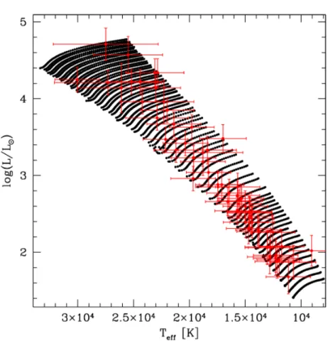
Fig. 2.— HR-diagram with the model grid for mode identification, as described in the text, denoted in black. The position of all treated B-stars together with their observational 2σ-error boxes are also shown in red.
Fig. 3.— Comparison between the amplitude ratios for two extreme β Cep models at the same position in the HR-diagram. The black lines denote the ratios for a model with initial metallicity Z = 0.01 and overshoot parameter αov = 0.5, the red lines are for Z = 0.02 and αov = 0.0. For both models, one theoretical eigenfrequency was selected in the β Cep interval with very similar values. In the plots for `=1, 2, 3 and 4 the red and black lines are almost indistinguishable.
B-stars in NGC 884. On the other hand, we note that Daszy´nska-Daszkiewicz et al. (2002) found large rotational effects on the amplitude ratios to be accompanied by large phase differences of the light curves in the different wavebands. We did not find any significant phase differences for the modes detected in our data, which points out that the effects of rotation, if any, are limited as they would otherwise result in measurable phase differences for the amplitudes in the different filters. Thus, as Balona et al. (1997), we perform the mode identification under the assumption that the rotation can be ignored in the computation of the theoretical amplitude ratios, realising that this may not be optimal for all the modes in all the considered pulsators.
5.2. Application to the B-stars in NGC 884
For each pulsator, models in the sub-grid in Fig. 2 that fitted the observed position in the HR-diagram within a 2σ-error box, as derived in Sect. 3 and noted in Table 1, Table 2 and the last column of Table 3, were retained. For each model and each degree `, we selected the eigenfrequencies fT,i that match the observed frequency fi ± 0.2 d−1. We take an uncertainty of 0.2 d−1 into account since the theoretical eigenfrequencies assume axisymmetric modes. We cannot compute a more exact value for the rotational splitting due to unknown inclination and rotation rate of the star, in combination with the unknown azimuthal number m. Our approach is stricter than in the previous applications mentioned above (De Cat et al. 2005, 2007; Handler et al. 2006, 2005) where the closest frequency in their used model grid, which was in addition much less dense than ours, was selected, irrespective of the difference with the theoretical frequency value. We have therefore followed a particularly conservative approach in assigning mode identifications to our detected frequencies.
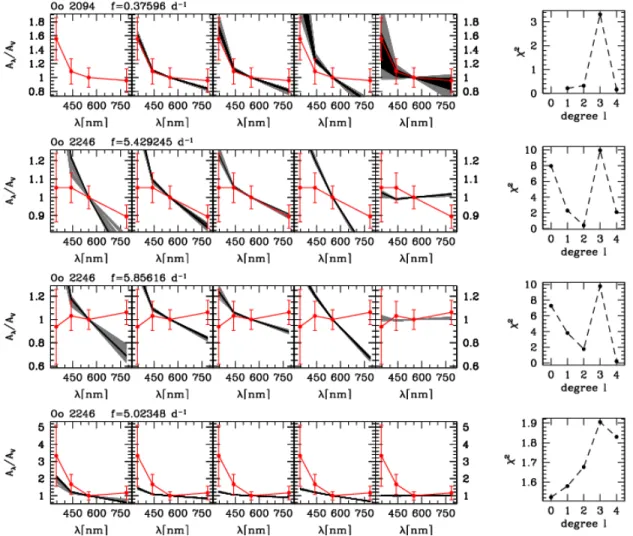
We confronted the theoretical amplitude ratios retained in this way with those observed. We illustrate the results of the mode identification by two examples. The outcome for all B-stars treated in this section can be found in Table 4 and Fig. 4. Our results rely on the selected sub-grid combined with the elimination of certain degrees ` for the 2σ-error box in the HR-diagram of each star as described in the previous paragraph. The results for Oo 2094 are based on the observed amplitude values presented in Table 4. The mode identification plots with the comparison between the theoretical and observational amplitude ratios are shown in the top left panel of Fig. 4. First of all, we eliminate the possibility of degree ` = 0. None of the models in the grid that fall in the 2σ-error box of Oo 2094 in the HR-diagram have (` = 0)-modes with frequencies close enough (± 0.2 d−1) to f1 = 0.37596 d−1. This is not at all surprising since the frequency value of f1already indicated that we are probably dealing with a g-mode. We can also eliminate `= 3, be-cause the theoretical amplitude ratios for the I filter never match the observed one within the uncertainties. We retain `= 1, 2 and 4, but remark that the observational amplitude ratios follow best the theoretical band for `= 4.
The mode identification for the three frequencies detected in Oo 2246, f1 = 5.429245 d−1, f2 = 5.85616 d−1and f3= 5.02348 d−1, is shown in the lower three left panels of Fig. 4. The observed amplitude ratios are only compatible with the theoretical models with ` = 2 for f1, ` = 4 for f2 and ` = 0 for f3,
Fig. 4.— (Left) Amplitude ratios scaled to the V filter for the frequency and the star denoted above the figure. The red filled circles with error bars denote the observed amplitude ratios and their uncertainties, the grey bands indicate the theoretical predictions for these, running from `= 0 at the left to ` = 4 at the right. The black bands denote a subsample of these theoretical models that deviate only 500 K in effective temperature and 0.05 dex in luminosity from the observed position in the HR-diagram. (Right) Corresponding χ2-value as a function of the degree `. (The mode identification plots for all stars and frequencies are available in the electronic edition of the journal.)
although the dependence of the observed ratios on wavelength does not always resemble the theoretical one. We also note that, even though we are just on the limit of eliminating the possibility of `= 1 for f3, there is not much reason to prefer `= 0 to ` = 1.
We also identified the mode degree from an alternative approach, as in, e.g., De Ridder et al. (2004); Handler et al. (2006), by calculating a χ2-value for every frequency and every degree `, as
χ2(`)= √ 1 N −1 N X j=1 Aj,th/AV,th− Aj,obs/AV,obs σj,obs !2 , (4)
with N the total number of filters available for the star and σj,obsthe error on the observed amplitude ratio for filter j (see also Aerts 2000; Aerts et al. 2010). The same models were selected as described above and the χ2-value for the best fitting model was retained for every degree, i.e., the mode with minimal χ2 is preferred. The outcome for the stars described above is shown in the right panels of Fig. 4 and the result is in agreement with the one of the left panels of these figures. The χ2-value indeed expresses the difference of the observed mean amplitude ratio to the one predicted from the closest model. There is no statistically founded acceptance criterion for such χ2-values. However, we note that in the examples above, the elimination process relying on the left panels often retains only models with χ2 < 1. We only use this χ2-value to prefer specific degrees ` when a clear minimum is visible, as noted in Table 4 by putting these `-values in bold. We remark that we always included the amplitudes in the U filter, when available, because, although their error is often larger than for the other filters, the calculated χ2-value accounts for this.
The results for all the mode identification attempts are represented in Fig. 4. For one star, Oo 2371, which has one frequency, we omitted the mode identification since it is an ellipsoidal binary. We securely identified the degree for 12 of the 114 detected frequencies: nine of the 64 investigated stars have at least one mode degree identified.The stars and frequencies for which we only retain one possibility for the degree ` of the modes, are the following: f1= 0.32811 d−1in Oo 2191 has `= 4, f2= 3.12734 d−1in Oo 2242 has `= 2, f1= 5.429245 d−1, f2= 5.85616 d−1and f3= 5.02348 d−1in Oo 2246 have ` = 2, 4 and 0, respectively, f1= 3.07229 d−1 in Oo 2262 has ` = 4, f1= 3.145150 d−1 in Oo 2299 has ` = 2, f1= 0.76570 d−1 in Oo 2372 has ` = 4, f1= 4.58161 d−1 in Oo 2444 has `= 1, f1= 6.16805 d−1in Oo 2488 has ` = 2, and f1= 4.41463 d−1and f2= 4.76330 d−1in Oo 2572 have ` = 2 and 1, respectively. The identified modes will turn out to be powerful input for the derivation of cluster properties as we show below. Nevertheless, the number of unambiguous mode identifications is low, in view of the immense observational effort put into the observing campaign. The lack of good photometric capabilities based on ultraviolet filters led to too uncertain amplitudes at blue wavelengths. This propagated to too high uncertainties for the amplitude ratios to be of sufficiently strong diagnostic value to identify the majority of the detected modes. Future campaigns should take this into account.
6. RESULTS FOR INDIVIDUAL STARS
In this section, we describe the results of the weighted analysis of the V, B, I and U light curves for individual stars and the mode identification of the detected frequencies. For figures of the light curves, the
phase diagram with the dominant frequency and the periodograms of the treated B-stars, we refer to the electronic appendix A of Saesen et al. (2010). A summary of the pulsational properties of all these stars, such as frequencies, amplitudes, phases and degrees ` of the modes, are noted in Table 4.
The manually performed frequency analysis of all these stars was done similarly as described in Sect. 4 for Oo 2444. In the following, the results of the non-weighted analysis of the V light curves are comparable to the weighted analysis, except if we state otherwise. When the data in a filter was too limited, or the harmonic fit was too bad, we did not note the results of the frequency fit for that filter. Some stars need some additional remarks, they are noted below, sorted on the star number.
The results of the mode identification were obtained in the same way as described in Sect. 5 for Oo 2094 and Oo 2246. We did not perform a mode identification for harmonic and combination frequencies, since the probability that they are independent frequencies is very small, as we have checked in our extensive grid of frequencies based on theoretical models, e.g., the probability for an independent harmonic frequency is about 2x10⁻⁴. In Table 4, we eliminated degree possibilities when no models were retained for the star and frequency of interest in the case of ` = 0 or when no theoretical amplitude ratios matched the observed ones within the uncertainties for the models selected within the 2σ-error box in the HR-diagram. We also evaluated the calculated χ2-value for the remaining degrees. When a specific degree was preferred based on its χ2-value, we stated so in Table 4 by putting its `-value in bold. Whenever no possibilities for ` = 0 to ` = 4 are left, it might be caused by ` > 4, as spectroscopic studies show that high-degree modes occur in moderately rotating pulsating B-stars (e.g., Aerts et al. 1998; Telting & Schrijvers 1998; Telting et al. 2001; Ausseloos et al. 2006). It could also be that the moderate rotation affects the observables too much such that the mode identification is erroneous, as pointed out by Handler et al. (2012), or that we are not dealing with a pulsation frequency. The mode identification figures for all the stars are shown in Fig. 4. The results of the mode identification in Table 4 should be regarded in combination with these figures, in order to interpret the magnitude of discrepancy between the models and observations.
Oo 1898
After optimisation of the light curves and a detailed frequency analysis, no significant frequency peaks could be found any more in star Oo 1898. We only retain a candidate frequency f = 3.648 d−1with a S/N of 3.9 in the V data.
Oo 1973
After optimisation of the light curves and a detailed frequency analysis, no significant frequency peaks could be found any more in star Oo 1973.
Oo 2086
For star Oo 2086 we find frequency values around 25 and 29 d−1, which are not at all expected for B-type pulsators. Based on its observed frequencies, this star is a δ Sct variable and thus not a cluster member, as already pointed out in Saesen et al. (2010).
Oo 2089
The analysis of Oo 2089 revealed only significant frequencies in the V filter. The frequency value of f2 is rather close to 1.003 d−1and so we have to be cautious since it may not be an intrinsic frequency.
Oo 2091
After prewhitening with f1and f2, we found an additional significant frequency f = 1.0437 d−1in the weighted and non-weighted analysis of the V residuals. To check whether this is an intrinsic frequency or not, we analysed the data of Białk´ow (Poland) and Xinglong (China) Observatory separately. Frequency f = 1.0437 d−1only shows up in the Białk´ow data and is totally absent in the Xinglong data. Therefore we do not accept this frequency. Prewhitening with f did not reveal any other significant frequencies, so we stopped the frequency search at this point.
Oo 2094
After removing a sine fit with the main frequency f1 and its harmonic f2 = 2 f1, we obtained the candidate frequency f = 0.479 d−1. This frequency is the highest peak in both the B and V periodograms of the residuals, but its amplitude does not exceed the needed signal-to-noise ratio to accept it formally, i.e., it has a S/N of 3.7 in V and of 3.4 in B.
Oo 2110
The two significant frequencies we accepted for Oo 2110 are f1 and f2. After prewhitening, a third significant frequency, f = 3.0231 d−1 showed up in the weighted and non-weighted analysis of the V data. This frequency was not present in the other filters. A separate analysis of the V data of different observatories, showed f in the Białk´ow, but not in the Xinglong data. Therefore we did not accept this third frequency as intrinsic for the time being.
Oo 2116
In Oo 2116 we can only detect one frequency f1. In the I data, the alias peak f10 = 4.21 d−1is higher, whereas in V and B, the peak at f1 itself is highest. Since the V data are less suffering from aliasing, according to the spectral windows, and since in both V and B data f1is highest, we believe this is the right peak.
Oo 2139
We cannot identify any significant peaks in Oo 2139, but the Fourier spectra of the data in the different filters are dominated by peaks in the range between 0.4 d−1and 0.6 d−1.
Oo 2146
Only in the V data of Oo 2146, a significant frequency can be detected: f = 4.013 d−1 with a S/N of 4.2. However, its value is equal to four times 1.0027 d−1within its error bars. Since the data for Oo 2146 mainly come from one observatory, Xinglong, we cannot conduct a further analysis to decide whether this frequency could be intrinsic to the star or not. Therefore we do not include it in a harmonic fit.
Oo 2185
For this star, no frequency could be accepted in the weighted analysis. Therefore, the parameters of the frequency fit noted in Table 4 are the results of a non-weighted analysis. In the weighted analysis, much importance is given to the precise Białk´ow data, which are spread over the three observing seasons, whereas the Xinglong data, spread over only four months, become important in the non-weighted analysis, due to their overwhelming number. This may be the reason why the non-weighted frequency search gives better results than the weighted one, since it is possible that the frequencies of Oo 2185 are not stable over time, due to its Be nature.
Oo 2189
After the time series optimisation, we do not find any significant frequencies any more in Oo 2189, except f = 0.10411 d−1that just reaches a S/N of 4 in a non-weighted analysis of the V data. This frequency, however, does not at all show up in a separate analysis of the Białk´ow and Xinglong data, and therefore we do not trust it.
Oo 2191
Oo 2191 was announced as candidate SPB star by Saesen et al. (2009) and the derivation of the two frequencies f1and f2confirms this pulsational behaviour.
Oo 2228
The results from the weighted and non-weighted frequency search for Oo 2228 are not the same. The first frequency in the weighted V analysis is f1 with a S/N of 4.5 and it is also marginally present in the I data. In the non-weighted V data we first retrieved f = 0.959 d−1, prewhitening for this frequency gives f = 2.778 d−1or f1. It is impossible to distinguish between these two values, so we have to be aware that we may not have taken the correct frequency peak. Prewhitening the weighted and non-weighted data set with f1gave no more significant frequencies, that differ enough from a multiple of 1 d−1and that are similar in both data sets. Therefore we only accept f1.
Oo 2235
After a carefully executed analysis of Oo 2235, we cannot find any significant frequencies in the dif-ferent filters, although the star surely is variable.
Oo 2242
Be-star Oo 2242 was discovered to be a variable star by Krzesi´nski & Pigulski (1997). Their data showed variations on a time-scale typical for λ Eri variables. Strong aliasing prevented them from giving the correct frequency peak.
With our data set, we were able to determine a first frequency peak at f1. The non-weighted V analysis led to a second significant frequency f2. Its value is very close to 2 f1. However, when we fixed the second frequency as harmonic 2 f1 in the sine fit, the amplitude of 2 f1 is much lower than the one for f2in the pe-riodogram and after prewhitening, we again obtained f2. Moreover, since the frequency difference between 2 f1 and f2 is nearly 4 year aliases, we also fitted ( f1− 2yr−1) and its first harmonic (2 f1 − 4yr−1) to the data. This time, the amplitude of ( f1− 2yr−1) was much lower than the one for f1and the amplitude of the harmonic (2 f1− 4yr−1) corresponded to the one of f2. Prewhitening gave again an additional frequency f1 with an amplitude as expected. This whole analysis points to f2being an independent additional frequency.
We also retrieved these two frequencies when combining our data set with the measurements of Krzesi´nski & Pigulski (1997). Since the time span of the data is much longer in this way, the frequency value can be deduced much more accurately. Therefore we adopted the non-weighted results of the combined data sets in Table 4.
Oo 2245
The periodograms of Oo 2245 in the different filters first showed many long periods, that were due to different zero points in the three observing seasons. After adjusting them, the low frequencies were absent in the V and U periodogram, but for the I and B data we needed to fit one low frequency to get to the intrinsic frequencies. After prewhitening with f1and f2, only peaks at multiples of 1 d−1appeared and we stopped the frequency analysis.
Oo 2246
Krzesi´nski & Pigulski (1997) discovered Oo 2246 as one of the two first β Cep stars in NGC 884. They could disentangle two frequencies in their data, that correspond with our f1 and f2. After prewhitening, we detected a third frequency f3 in the B data. We optimised all three frequencies in the B filter, after verifying that the frequency values of f1and f2 are the same as the optimised V values within their error bars. Combining our light curve with the one from Krzesi´nski & Pigulski (1997) reproduced the same frequencies. Due to the longer time span, the results shown in Table 4 are thus obtained in the joined data sets.
Oo 2253
Oo 2253 was reported as SPB candidate by Saesen et al. (2009) and they extracted three significant frequencies in the data of Białk´ow and Xinglong Observatory. We confirm here their first two frequencies, denoted as f1and f2in Table 4, but we do not detect their third frequency in our merged data set.
Oo 2267
After prewhitening for f1and f2, we found a candidate frequency f = 4.546 d−1in the I residuals. This frequency has a S/N of 3.3 in B, 3.4 in V and 3.7 in I, which is not high enough to accept it. Moreover, due to strong aliasing, we cannot be sure to have picked out the correct frequency peak.
Oo 2299
Oo 2299 was discovered as candidate variable star on a time scale of six hours by Percy (1972) and was identified as second β Cep star in NGC 884 by Krzesi´nski & Pigulski (1997). They report a single periodicity at f1. With our data set we cannot detect any other frequencies within the detection threshold either. The results noted in Table 4 originate from the combined data set.
Oo 2319
Two significant intrinsic frequencies, f1and its harmonic f2 = 2 f1were derived for Oo 2319. Prewhiten-ing gave alias structures of low frequencies, which we did not accept. We searched further, but no other significant peaks emerged.
The phases of f1 and f2 are the same in the different filters. The amplitude of f1 in U seems largest, and the one in I smallest, which is a typical signature for pulsations in B-stars. However, they do not differ within their error bars, therefore we cannot formally exclude the possibility that this star is an ellipsoidal binary.
Oo 2324
Prewhitening Oo 2324 with f1and f2, gives a nice peak at f3with a S/N = 5.6 in the weighted analysis of the V residuals. In the other filters, aliasing and higher noise levels hamper the detection of other frequency peaks. The frequency value of f3is close to 3 times 1.0027 d−1, so we should be careful with it. However, when analysing V data of Białk´ow and Xinglong Observatory separately, both sites indicate f3as significant frequency. Therefore we are inclined to accept it as intrinsic frequency. Further prewhitening no longer gave significant frequency peaks.
Oo 2345
The first frequency found in the data of Oo 2345 is very close to 2 d−1. We retrieved f1 in all filters, and also in the analysis of some observatories separately. A phase diagram folded with this frequency, as shown in Fig. A.37 of Saesen et al. (2010), displays a clear sinusoidal variation. We are thus inclined to accept f1as intrinsic frequency of Oo 2345. Removing a sine fit with f1reveals another frequency f2, which is present in the B, V and I residuals. Hereafter no more frequency peaks were accepted.
Oo 2371
Oo 2371 is an ellipsoidal binary with orbital period around 5.2 d. The binary star was first discovered as candidate by Krzesi´nski & Pigulski (1997) and later confirmed in spectroscopic data by Malchenko (2007). Our deduced frequency f1 is, as expected, twice the orbital frequency and the amplitudes in the different filters indeed do not follow the typical relation for B-type pulsations. We also note that a frequency analysis in the different observing seasons showed evidence for a changing amplitude over time, pointing to an interacting binary due to a close orbit (Malchenko 2007). In Table 4 we note the frequency as found in the combined data set. We did not execute a mode identification for this star, since we are not dealing with pulsations.
Oo 2406
Frequency f1 is significant in the V and I data of Oo 2406. Prewhitening shows the presence of a second frequency peak, both in the V and I residuals, but with a different alias frequency. I data suffer more from aliasing than V data and so the difference between both peaks is significantly less than for the V filter. Therefore we adopt f2given by the V residuals as the correct frequency peak.
Oo 2426
After optimisation of the light curves in the different filters and a detailed frequency analysis, we do not recover any significant frequencies for star Oo 2426.
Oo 2429
For Oo 2429, the results noted in Table 4 were optimised in the B filter, since this filter led to more significant frequencies. Moreover, optimising f1in the B filter resulted in the same frequency values within the error as optimising in V.
Oo 2448
The results obtained for Oo 2448 should be treated with caution: the periodograms suffered from severe aliasing. We adopted the frequencies coming from the B periodograms, since its alias frequency was lower than for the V data, as in the spectral window. The highest peaks in V are f10 = 0.497 d−1and f20 = 2.430 d−1 with a S/N of 4.0 and 4.8, respectively.
Oo 2488
Oo 2488 was for the first time announced as variable star with β Cep-like oscillations by Pigulski et al. (2007) in a preliminary report on the multi-site campaign on NGC 884. Saesen et al. (2008) derived two significant frequencies, f1 and f2, in a frequency analysis on the single-site data of Białk´ow Observatory. An analysis of the bi-site data of Białk´ow and Xinglong Observatory by Saesen et al. (2009) led to the same two frequencies. An analysis of the total data set, as carried out here, confirms f1and f2and even permits the detection of a third frequency f3.
Oo 2462
As for star Oo 2185, no frequencies could be accepted in a weighted analysis, so that the results in Table 4 come from a non-weighted frequency analysis.
Oo 2562
After prewhitening with significant frequencies f1and f2, a third frequency f3is retrieved in the I data with a S/N of 4.6. Inclusion of this frequency and optimisation in the I filter do not change the harmonic fit for the two first frequencies in any of the filters. Given the large errors, the parameters of the harmonic fit for this third frequency as noted in table 4 cannot be trusted.
Oo 2566
Pigulski et al. (2007) and Saesen et al. (2008) already mentioned Oo 2566 as candidate β Cep star based on (a part of) the first season Białk´ow data. A frequency analysis on the whole campaign data set is suffering from long-term variations caused by the Be-character of the star. Frequency f1, however, recurs in the V, B an U data after removing some arbitrary low frequencies, but is only significant in the V data. Since the chaotic behaviour of this Be-star hampers our time series analysis, the results in Table 4 should be taken with caution.
Oo 2572
Oo 2572 was discovered and analysed in the same preliminary reports on the multi-site campaign as for Oo 2488. Saesen et al. (2009) remarked that the analysis of the bi-site data already was important in order to pinpoint the correct frequency peak, in comparison with the single site data. They derived two frequencies, f1 and f2, and reported that there is still power present in the residuals, but that no other frequency value could be determined.
We confirm these two frequencies in the frequency search in the whole campaign data set and retrieve a third frequency peak f3. After prewhitening with f1, f2 and f3, no other frequencies can be accepted for Oo 2572. Only in the non-weighted analysis of the V data, we find evidence for a candidate frequency
f = 4.389 d−1with a signal-to-noise level of 3.9.
Oo 2579
since they suffered severely from long-term effects hampering the detection of f1. For the other filters, Białk´ow data could be included.
Oo 2616
After prewhitening the B data of Oo 2616 with f1, a second frequency f2 is found on the limit of acceptance, i.e., with a S/N-level of 4.0. This frequency was also visible in the first periodogram of the V and I data and therefore we accept it and include it in the harmonic fit. The parameters of the harmonic fit were optimised in the B filter, but we have no high confidence in them due to their high error bars.
Oo 2622
Oo 2622 is definitely a variable star, as clearly seen in the V, B, and I light curves. However, residual trends hamper a clear and coherent frequency determination in the different filters. Therefore we do not attempt a harmonic fit for this star.
Oo 2649
We can only accept one frequency in the Be-star Oo 2649. However, the phase diagram folded with this frequency (see Fig. A.59 in Saesen et al. 2010) clearly shows additional variations. A possible candidate frequency is f = 2.264 d−1, which is clearly the highest peak in the V periodogram of the residuals, but its amplitude does not fulfill the signal-to-noise criteria to accept it.
Oo 2694
For Oo 2694 only one frequency, f1 can be accepted, but surely more variation is still hidden in the residuals. The residuals in the different filters pointed towards a different frequency peak, the one in the V data is most significant, at f = 1.502 d−1 or one of its aliases, with a S/N = 3.8. We cannot accept this frequency, but prewhitening with it even reveals more candidate frequencies. However, we cannot retrieve a trustable value for them, so we stopped the frequency search at this point.
Oo 2752
No significant frequencies can be found in Oo 2752 after optimisation of the light curves. We only retain one candidate frequency f = 1.811 d−1that has a S/N of 3.9 in the V data, which is not high enough to formally accept it.
Oo 2752
Only one frequency just reaches the 4.0 S/N-level in the V data of Oo 2752, namely f = 5.991 d−1. However, because of its closeness to 6 d−1, the S/N-level of the peak and the absence of proof in the other filters, we do not accept this frequency.
7. ADDITIONAL SEISMIC RESULTS
7.1. Relations between Pulsation and Basic Stellar Parameters
In this section, we do not consider star Oo 2371, since it is an ellipsoidal binary and not a pulsating star. We also exclude Oo 2086 and Oo 2633, which are, according to their frequency spectra, δ Sct stars rather than members of the cluster. This also means that their deduced position in the HR-diagram of Sect. 3 cannot be trusted. All other 62 B-stars that have at least one accepted frequency in Table 4 can be considered members of NGC 884 based on the photometric diagrams presented in Appendix A of Saesen et al. (2010). Slesnick et al. (2002), Uribe et al. (2002) and Currie et al. (2010) also investigated the membership of (some) of these periodic B-stars in detail, and all of them are believed to be a member star of NGC 884 by at least one of these sources.
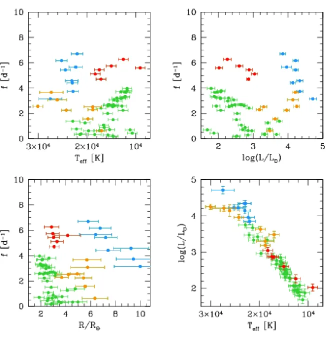
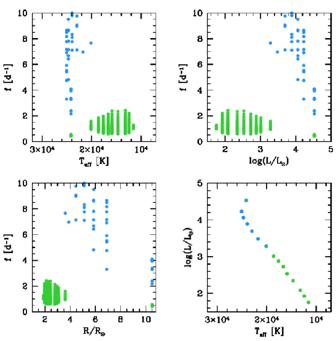
In Fig. 5 we show the frequency with the highest amplitude for every star with respect to the basic stellar parameters, log(L/L ), Teff and the radius R of the star. The latter was determined as (R/R )2 = (L/L )(Teff/Teff, )−4. We attributed different colours to different apparent groups in these diagrams, espe-cially on the basis of the radius. We used these figures to make a selection of the most appropriate stars for asteroseismology by visual inspection. Fig. 6 shows the theoretical analogue of the observational Fig. 5 for axisymmetric modes and is based on cl´es models with parameters X = 0.70, Z = 0.02, αov = 0.2 and log(age/yr)= 7.1 (Southworth et al. 2004b). We selected all theoretical eigenfrequencies with degrees ` = 0, 1 and 2 for p- and g-modes that are excited (a lower Z would result in less excited frequencies). In this way, we identify the blue observational group as p-mode pulsators and the green one as g-mode pulsators. The group in between, denoted in orange, contains all Be-pulsators amongst the studied B-stars. The stars denoted in red also reside between the p- and g-modes, but these are not known as Be-stars nor do we know their rotational velocities. On the basis of this comparison between observational and theoretical frequen-cies, we identify eight β Cep pulsators in the cluster: Oo 2246, Oo 2299, Oo 2444, Oo 2488, Oo 2520, Oo 2572, Oo 2601 and Oo 2694.
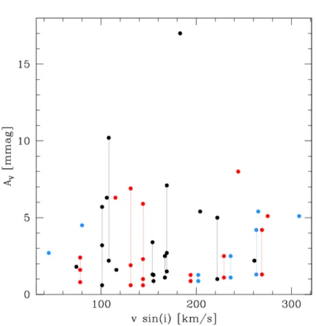
In Fig. 7 we show the amplitudes in the V filter of all observed frequencies for all B-stars with respect to the projected rotational velocities of Strom et al. (2005), Huang & Gies (2006), and Marsh Boyer et al. (2012) for all stars for which these data are available. Stankov & Handler (2005) found that slowly-rotating Galactic β Cep stars tend to have higher pulsation amplitudes, lending support to the hypothesis that rotation would act as an amplitude limiting mechanism. We do not find a clear connection between the observed rotation velocities and the mode amplitudes. We also note that our observed amplitudes are in general lower than the ones of the stars treated in Stankov & Handler (2005). We do not find any dependency either
Fig. 5.— Dominant frequencies for all B-stars with respect to the basic stellar parameters Teff, log(L/L ) and R, with their 1σ-error. The error on the frequency is smaller than the used symbol. Different colours are attributed to different apparent groups in the (R, f )-diagram (see Sect. 7.1). The bottom right figure shows all these stars in the HR-diagram.
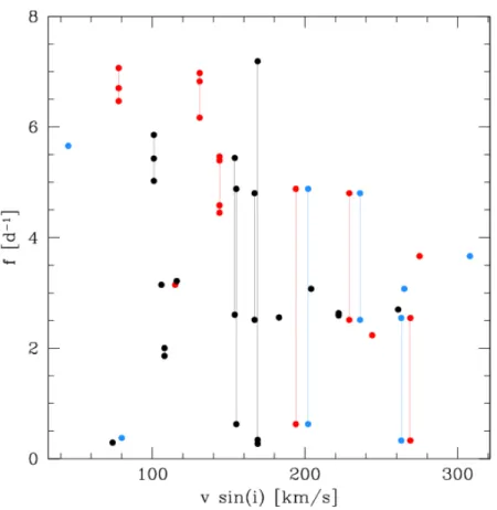
between the projected rotational velocities and observed frequencies, as shown in Fig. 8, but the V amplitude seems to get lower for higher frequencies, as shown in Fig. 9.
Fig. 6.— Same as Fig. 5, but for the excited theoretical eigenfrequencies of axisymmetric modes of degree ` = 0, 1 and 2 calculated for cl´es models with X = 0.70, Z = 0.02, αov = 0.2 and log(age/yr) = 7.1. The green points denote the g-modes, the blue points the p-modes.
7.2. Asteroseismology of the B-stars in the Cluster
We subsequently conducted a comparison between the observed frequencies of the eight selected β Cep stars and those that occur for our dense full grid of stellar models, to see whether we can find a consistent
Fig. 7.— Amplitude in the V filter of all observed frequencies with respect to the projected rotational velocities of Strom et al. (2005) (black points), Huang & Gies (2006) (red points), and Marsh Boyer et al. (2012) (blue points) for all stars for which these data are available. The amplitudes originating from the same star are connected.
Fig. 8.— All observed frequency values with respect to the projected rotational velocities of Strom et al. (2005) (black points), Huang & Gies (2006) (red points), and Marsh Boyer et al. (2012) (blue points) for all stars for which these data are available. The frequencies observed in the same star are connected.
Fig. 9.— All observed frequency values with respect to their V amplitude. For clarity we left out two points situated at ( f , AV) = (0.20871 d−1, 56 mmag) and ( f, AV)= (11.951 d−1, 1 mmag). The used colour code is the same as for Fig. 5 and is explained in Sect. 7.1.