HAL Id: pastel-00003009
https://pastel.archives-ouvertes.fr/pastel-00003009
Submitted on 24 Oct 2007
HAL is a multi-disciplinary open access
archive for the deposit and dissemination of
sci-entific research documents, whether they are
pub-lished or not. The documents may come from
teaching and research institutions in France or
abroad, or from public or private research centers.
L’archive ouverte pluridisciplinaire HAL, est
destinée au dépôt et à la diffusion de documents
scientifiques de niveau recherche, publiés ou non,
émanant des établissements d’enseignement et de
recherche français ou étrangers, des laboratoires
publics ou privés.
Evaluation analytique des performanes des réseaux
sans-fil par un processus de Markov spatial prenant en
compte leur géométrie, leur dynamique et leurs
algorithmes de contrôle
Mohamed Kadhem Karray
To cite this version:
Mohamed Kadhem Karray. Evaluation analytique des performanes des réseaux sans-fil par un
pro-cessus de Markov spatial prenant en compte leur géométrie, leur dynamique et leurs algorithmes de
contrôle. domain_other. Télécom ParisTech, 2007. English. �pastel-00003009�
´
Ecole Nationale Sup´erieure des T´el´ecommunications ´
Ecole Doctorale d’Informatique, T´el´ecommunications et ´Electronique
Thesis: Analytic evaluation of wireless cellular
networks performance by a spatial Markov
process accounting for their geometry, dynamics
and control schemes
Informatique et R´eseaux
Mohamed Kadhem KARRAY
Jury: Zwi Altman (HDR, France Telecom R&D) examiner
Fran¸cois Baccelli (Professor, INRIA)
BartÃlomiej BÃlaszczyszyn (Doctor, INRIA) thesis supervisor
David MacDonald (Professor, University of Ottawa) examiner
Laurent Massouli´e (Doctor, Thomson Research) examiner
–contresigned by Laurent Viennot (HDR, INRIA)–
Eric Moulines (Professor, ENST) thesis supervisor
Contents
Preface ix
Abstract xi
Introduction xiii
0.1 Problem statement . . . xiii
0.2 Objectives . . . xvi
0.3 Organization . . . xvii
0.4 Publications . . . xvii
I
Feasibility based load control
1
1 Introduction 3 1.1 Related works . . . 31.2 Our contribution . . . 5
1.3 Organization . . . 6
2 Preliminaries 7 2.1 Single link performance . . . 7
2.2 Model . . . 9
2.2.1 Multiple access . . . 9
2.2.2 Cell pattern . . . 9
2.2.3 Propagation . . . 11
2.2.4 Antennas . . . 11
2.2.5 UMTS numerical parameters . . . 12
2.3 Notation . . . 14
2.3.1 Antenna locations and path loss . . . 14
2.3.2 Engineering parameters . . . 15
2.3.3 Mathematics . . . 16
3 Feasibility conditions 17 3.1 Downlink . . . 17
3.1.1 Power allocation problem . . . 18
3.1.2 Feasibility conditions . . . 22 iii
iv CONTENTS
3.2 Uplink . . . 24
3.2.1 Power allocation problem . . . 24
3.2.2 Feasibility conditions . . . 31
3.3 Admission control schemes . . . 33
4 First performance evaluation 35 4.1 Mean model . . . 35 4.1.1 Downlink . . . 36 4.1.2 Uplink . . . 38 4.2 Infeasibility probability . . . 39 4.2.1 Calculation methods . . . 40 4.3 Numerical results . . . 42
II
Spatial Markov Queueing
45
5 Introduction 47 5.1 Related works . . . 475.2 Our contribution . . . 48
5.3 Organization . . . 48
6 Spatial Markov queueing process (SMQ) 49 6.1 Preliminaries . . . 49
6.1.1 Point process . . . 49
6.1.2 Measure-valued Markov process . . . 51
6.2 Spatial Markov queueing process . . . 53
6.2.1 Infinitesimal generator . . . 54
6.2.2 Regularity . . . 56
6.2.3 Interpretation of Whittle SMQ . . . 62
6.3 Limiting behavior . . . 63
6.3.1 Limiting distribution . . . 63
6.3.2 Novelty of our ergodicity conditions . . . 68
6.3.3 Invariance of the limiting distribution . . . 71
6.3.4 Time averages . . . 73
6.3.5 Countable case . . . 76
6.4 Invariant probability measure . . . 76
6.4.1 Balance for Whittle SMQ . . . 77
6.4.2 Balance for SMQ . . . 81
6.4.3 Invariant probability measure . . . 82
6.5 Mobility process for wireless networks . . . 83
6.5.1 Completely aimless mobility . . . 83
6.5.2 Intracell mobility . . . 84
6.5.3 Intercell mobility . . . 88
CONTENTS v
7 SMQ for elastic traffic 91
7.1 Whittle model . . . 91
7.1.1 Model . . . 91
7.1.2 Service rate balance . . . 93
7.1.3 Ergodicity . . . 94
7.1.4 Performance . . . 97
7.2 Wireless model . . . 102
7.2.1 Model . . . 102
7.2.2 Service rate balance . . . 103
7.2.3 Ergodicity . . . 104
7.2.4 Performance . . . 107
8 SMQ for streaming traffic 111 8.1 Whittle and wireless models . . . 112
8.1.1 Whittle model . . . 112
8.1.2 Wireless model . . . 114
8.2 Two spatial loss wireless models . . . 116
8.2.1 Transition blocking model . . . 118
8.2.2 Forced termination model . . . 123
8.2.3 Approximation of the cut probability . . . 125
III
Performance evaluation
129
9 Introduction 131 10 UMTS Release 99 133 10.1 Introduction . . . 133 10.2 Elastic traffic on DSCH . . . 133 10.2.1 Related works . . . 133 10.2.2 Our contribution . . . 13410.2.3 Congestion control algorithms . . . 134
10.2.4 Associated SMQ process . . . 136
10.2.5 No mobility case . . . 137
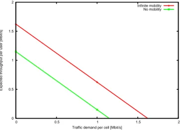
10.2.6 Infinite mobility case . . . 139
10.2.7 Numerical results . . . 140
10.3 Streaming traffic on DCH without mobility . . . 146
10.3.1 Related works . . . 146
10.3.2 Our contribution . . . 148
10.3.3 Associated SMQ process . . . 148
10.3.4 Calculation methods . . . 152
10.3.5 Numerical results . . . 153
10.4 Streaming traffic on DCH with mobility . . . 153
10.4.1 Related works . . . 154
10.4.2 Our contribution . . . 155
vi CONTENTS
10.4.4 Numerical results . . . 159
10.5 Integration of elastic and streaming traffic . . . 160
10.5.1 Related works . . . 161 10.5.2 Our contribution . . . 163 10.5.3 Traffic model . . . 164 10.5.4 Performance analysis . . . 164 10.5.5 Numerical results . . . 168 11 HSDPA 173 11.1 From link level to dynamic system level . . . 173
11.1.1 Link level . . . 173
11.1.2 From link level to static system level . . . 174
11.1.3 From static to dynamic system level . . . 177
11.1.4 Comparing DSCH and HSDPA . . . 177
11.2 Numerical results . . . 177
11.3 HSDPA scheduler performance . . . 178
12 GSM 183 12.1 Introduction . . . 183 12.2 Model . . . 183 12.2.1 GSM versus UMTS . . . 184 12.2.2 FDMA . . . 185 12.2.3 Traffic . . . 186 12.2.4 Frequency hopping . . . 187
12.3 Power allocation feasibility . . . 188
12.3.1 Power allocation problem . . . 188
12.3.2 FC . . . 189 12.4 Numerical results . . . 190 12.5 Conclusion . . . 190
IV
Conclusion
193
12.6 Summary of Contributions . . . 196 12.7 Future Research . . . 197V
Appendices
199
13 Appendix of Part I 201 13.A Power allocation basic results . . . 20113.A.1 Power allocation problem . . . 201
13.A.2 Feasibility . . . 202
13.A.3 Minimal solution . . . 204
13.B The f-factor . . . 209
13.B.1 Gain-sum . . . 209
CONTENTS vii 13.C Directional antennas . . . 220 13.C.1 The f-factor . . . 221 13.C.2 Mean model . . . 225 13.C.3 Infeasibility probability . . . 226 13.D Synthesis of formulae . . . 227
13.E Comparison of admission control schemes . . . 229
13.E.1 Constructor’s schemes . . . 230
13.E.2 Comparison in a semi-dynamic context . . . 231
13.E.3 Comparison in a dynamic context . . . 235
14 Appendix of Part II 239 14.A Classical queues . . . 239
14.A.1 M/GI/1/PS . . . 239
14.A.2 M/GI/∞ and loss queue . . . 242
14.B Fairness . . . 244
14.B.1 Definitions . . . 245
14.B.2 Basic properties . . . 245
14.B.3 Max-min fairness . . . 248
Preface
I wish to thank my family, my parents, my brothers and my sister, my wife and my daughter, and also my friends who support and encourage me throughout the duration of my thesis.
I am particularly honored to have been able to collaborate with professor Fran¸cois Baccelli and doctor Bartek BÃlaszczyszyn, from INRIA1& ENS2, while
writing my thesis; I hope to continue this fruitful collaboration. I wish to thank my supervisors professor Eric Moulines, from ENST3 and doctor Bartek
BÃlaszczyszyn, for their encouragement and advise. I am particularly grateful to professor Pierre Br´emaud for his rich lectures on “Signal, Information and Communication” at ENS. I wish also to thank the referee and examiners for reading the thesis and their suggestions. I particularly thank professor David McDonald and doctor Laurent Massouli´e who accept to review my report, doc-tor Zwi Altman for his encouragements throughout the duration of my thesis and mister Omar Soufit for his fruitful collaboration particularly in the simula-tions. Thanks also to my colleagues at France Telecom who supplied me with interesting problems and relevant information.
1Institut National de Recherche en Informatique et en Automatique 2Ecole Normale Sup´erieure
3Ecole Nationale Sup´erieure des T´el´ecommunications
x PREFACE
Short abstract: We build load control schemes for wireless cellular networks and develop analytic methods for the performance evaluation of these networks by a spa-tial Markov process accounting for their geometry, dynamics and control schemes. First, we characterize the single link performance by using the digital communication techniques. Then the interactions between the links are taken into account by for-mulating a power allocation problem. We propose decentralized load control schemes which take into account the influence of geometry on the combination of inter-cell and intra-cell interferences. In order to study the performance of these schemes, we analyze a pure-jump Markov generator that can be seen as a generalization of the spatial birth-and-death generator, which allows for mobility of particles. We give suf-ficient conditions for the regularity of the generator (i.e., uniqueness of the associated Markov process) as well as for its ergodicity. Finally we apply our spatial Markov process model to evaluate the performance of wireless cellular networks using the fea-sibility based load control schemes.
Keywords: wireless, cellular, performance, load control, power allocation feasibility, birth-and-death, mobility, regularity, ergodicity, invariant measure, Gibbs, spatial Er-lang formula, blocking, cut probability, delay, throughput.
Titre (in frensh): Evaluation analytique des performances des r´eseaux cellulaires sans fil par un processus de Markov spatial prenant en compte leur g´eom´etrie, dy-namique et algorithmes de contrˆole
Cour r´esum´e: Nous proposons des algorithmes de contrˆole de charge pour les r´eseaux cellulaires sans fil et d´eveloppons des m´ethodes analytiques pour l’´evaluation des performances de ces r´eseaux par un processus de Markov spatial prenant en compte leur g´eom´etrie, dynamique et algorithmes de contrˆole. D’abord, nous caract´erisons la performnace d’un lien unique en utilisant les techniques de communication num´erique. Ensuite les interactions entre les liens sont prises en compte en formulant un probl`eme d’allocation de puissances. Nous proposons des algorithmes de contrˆole de charge d´ecentralis´es qui tiennent compte de l’influence de la g´eom´etrie sur la combinaison des interf´erences inter-cellules et intra-cellules. Afin d’´etudier les performances de ces algorithmes, nous analysons un g´en´erateur d’un processus Markovien de saut qui peut ˆetre vu comme une g´en´eralisation du g´en´erateur de naissance-et-mort spatial, qui tient compte de la mobilit´e des particules. Nous donnons des conditions suffisantes pour la r´egularit´e du g´en´erateur (c.-`a-d., unicit´e du processus de Markov associ´e) aussi bien que pour son ergodicit´e. Enfin nous appliquons notre processus de Markov spatial pour ´evaluer les performances des r´eseaux cellulaires sans fil utilisant les algorithmes de contrˆole de charge bas´es sur la faisabilit´e de l’allocation de puissance.
Mots-cl´es: sans fil, cellulaire, performance, contrˆole de charge, faisabilit´e de l’allocation de puissance, naissance-et-mort, mobilit´e, r´egularit´e, ergodicit´e, mesure invariable, Gibbs, formule d’Erlang spatiale, blocage, probabilit´e de coupure, delai, d´ebit.
Abstract
We build load control schemes for wireless cellular networks which are rapid and efficient and develop analytic methods for the performance evaluation of these networks by a spatial Markov process accounting for their geometry, dynamics and control schemes. We show that the analytic evaluation of the performance of wireless cellular networks is possible, but it requires the use of tools coming from several disciplines.
The first step is to characterize the single link performance by using the digital communication techniques. Then the interactions between the links are taken into account by formulating a power allocation problem. Optimal load control schemes based on the necessary and sufficient condition for the feasibility of the power allocation problem are unpractical because they are centralized. Extending the work in [16], we propose load control schemes that allow each base station to decide independently of the others what set of voice calls to serve and/or what bit rates to offer to elastic calls competing for bandwidth. These control schemes are primarily meant for large CDMA networks. They take into account in an exact way the influence of geometry on the combination of inter-cell and intra-cell interferences as well as the existence of maximal power constraints of the base stations and users. We also evaluate the performance of these control schemes in terms of the infeasibility probability (the probability that the admission’s condition doesn’t hold for a given cell when the calls are modelled as a Poisson process).
From the user’s point of view, the performance is more suitably evaluated by the mean of the blocking and cut (drop) probabilities of streaming (real-time as voice) calls and the delay and throughput of elastic (non-real-(real-time as web surfing) calls in the long run of the network. In order to build analytic methods for evaluating these performance indicators we build and analyze a pure-jump Markov generator that can be seen as a generalization of the spa-tial birth-and-death generator, which allows for mobility of particles. We give sufficient conditions for the regularity of the generator (i.e., uniqueness of the associated Markov process) as well as for its ergodicity. We show when the sta-tionary distribution is a Gibbs measure. This extends previous work in [97] by allowing for mobility of particles. Our spatial birth-mobility-and-death process can be seen also as a generalization of the spatial queueing process considered in [106, 67]. This way our approach yields regularity conditions and alterna-tive conditions for ergodicity of spatial open Whittle networks, complementing
xii ABSTRACT
works in [106, 67].
Next we apply our spatial Markov queueing process model to build analytical methods for evaluating the performance of wireless cellular networks controlled by feasibility based load control schemes. This evaluation is made by the mean of indicators which are relevant from the user’s point of view rather than the classical outage probability [47]. Our formula for the blocking probability of streaming traffic might be seen as a spatial extension of the well-known Erlang loss formula. In the case of elastic traffic, we build explicit analytic expressions for the user throughput.
The analytic performance evaluation permit to build a new class of coher-ent methods for the differcoher-ent fundamcoher-ental problems in wireless cellular systems: quality of service, capacity, dimensioning and cost. The ease of use of the ana-lytical expressions makes this type of approach more effective than simulations for macroscopic evaluation and optimization.
Introduction
Our research stems from wireless cellular communications which are in perma-nent and rapid evolution. In few years, wireless cellular systems have evolved through several generations with completely different characteristics (for exam-ple, different multiple access schemes: FDMA4 for GSM5, CDMA6 for UMTS7,
TDMA8 for HSDPA9). This rapid evolution explains perhaps why much of the
global performance analysis of these networks is made by simulations. Unfortunately, simulations give numerical result for a given situation but don’t give a global comprehension of the key parameters and relationships.
0.1
Problem statement
The performance evaluation of wireless cellular networks, is a hard task. First, the performance evaluation of a single radio link is difficult because we should take into account the radio signal variations due to multi-path fading. Moreover the signal processing techniques, such as modulation, spreading and power con-trol, etc., used to counteract the harmful effects of the radio signal variations are often complex (cf. for example [51, Chapter 9], [118, §3.4.3]).
Once the single link performance evaluation is carried, we should take into account the interference between the different links which depends on the rela-tive geographic positions of the users. This process is usual in the engineering of the wireless cellular networks; first we characterize the performance of a sin-gle link and in a second step we consider the interactions between the different links. In doing so, we should consider carefully the separation of the time scales between phenomena such as multi-path fading and variations due to the geome-try of the problem. (We will see an example of this issue when we study HSDPA later.) This is not an easy task as it depends not only on the phenomenon itself but also on the control algorithms (e.g. power control) in the network.
Wireless networks have to offer service for calls (users) which have differ-ent requiremdiffer-ents and which may be roughly classified in two classes:
4Frequency Division Multiple Access 5Global System for Mobile
6Code Division Multiple Access
7Universal Mobile Telecommunications System 8Time Division Multiple Access
9High Speed Downlink Packet Access
xiv INTRODUCTION • Real-time (or streaming) calls (voice calls, real-time audio-video
stream-ing) require a fixed bit-rate on each link, and they are blocked if momen-tarily it is not possible to satisfy their requirement. To analyze the quality offred to such calls, one constructs loss models and studies blocking and cut (drop) probabilities.
• Non-real-time (or elastic) calls (data traffic) can be served at an
ar-bitrary low bit-rate, for the price of large delays. To analyze the quality offred to such calls, one uses typically queueing models and studies sojourn times (delays) and average throughput.
The interaction between all the users is taken into account in specific control schemes called load control schemes, which may be roughly classified in two types: admission control for streaming calls and congestion control for elastic ones. These load control schemes attempt to assure that the required performance specific to each single radio link is satisfied. More precisely they manage traffic in order to ensure required quality for both incoming calls as well as previously admitted ones, and to reject incoming calls only when necessary. The essential problem for the load control decisions may be formulated as fol-lows: may the network allocate a power to each user large enough for him to get his required link performance and small enough for the other users to get their required link performance. We say that load control attempt to ensure the feasibility of the power allocation problem, and if so, the user powers may be found by an iterative process called power control. Solving the power control problem isn’t in the scope of the present work (cf. for example [55] and the references therein). We will focus only on criteria which indicate if the power control problem is feasible or not, without trying to solve it.
One may consider a load control scheme based on the necessary and suffi-cient condition (denoted NSFC) of the feasibility of the power allocation prob-lem. Such load control scheme is optimal (i.e. offers the maximal capacity) but is unfortunately difficult to implement in real networks as the admission decision of a new call requires the collection and treatment of information from all the calls in the network. We call such load control scheme centralized. Moreover the performance evaluation of the optimal load control scheme is time consuming numerically, and hard analytically (no explicit formulae exist to our knowledge). The load control schemes implemented in the real networks are proposed by constructors (manufacturers) [64], [81]. They are decentral-ized (i.e. depend on parameters which are local to the cell in which the new call request for admission) but they don’t assure the power allocation feasibility. Moreover no analytic evaluation method of the constructor schemes exist to our knowledge.
There is a rich literature on the performance evaluation of load control schemes in cellular networks. Unfortunately it is often difficult to find the rela-tionship between the indicators calculated by the authors because they consider different traffic models. The distinction between the following four classes of traffic models allows a first classification.
0.1. PROBLEM STATEMENT xv
• Static model: Number and positioning of active (i.e. currently being
served) calls are fixed.
• Semi-static model: Active calls are modelled by a spatial Poisson point
process. In other words, “snapshots” of active calls are seen as realizations of spatial Poisson processes; these snapshots are used as the non-constrained traffic process on which we will define and evaluate the (in)feasibility prob-abilities.
• Semi-dynamic model: Users (or calls) arrive at a random location and
last for some random duration; each user is motionless during its call; this is the “minimal” dynamic model where an admission control can be specified, and where blocking probabilities can be considered.
• Dynamic model: We have the same as above but users may move during
their calls; an admission and motion (or handoff) control can then be specified. Blocking and motion-cut probabilities can be evaluated. The load control scheme performance may be evaluated by modelling the users as a planer Poisson process. This lead in the classical literature to the notion of outage probability [47], which is roughly the probability that a given user doesn’t attain his required link performance. The outage probability is not a satisfying performance indicator because it relies on some simplifying assumptions (especially on the powers of the users) which makes its meaning unclear. Another approximate method consists of making some average calculus leading in the classical literature to the notion of pole capacity. Both the outage probability and pole capacity are heuristics, and we consider in the present work more relevent performance indicators.
From the user’s point of view, the performance is more suitably eval-uated by means of the long run blocking and cut probabilities for streaming calls and the delay and throughput for elastic calls. Recall that the blocking probability is defined as the fraction of calls that are rejected by the admis-sion control scheme in the long run, a notion of central practical importance. (Analogous definitions may be formulated for the other indicators.) In order to calculate these dynamic performance indicators (blocking, cut, delay and throughput) we should consider the temporal dynamics and the geometry (lo-calizations) of the call arrivals, mobility and departures from the network. The temporal dynamics of the call arrivals and departures are well studied in wired communication networks, which led in particular to the famous (and widely used) Erlang’s formula [44]. This formula is often used for wireless cellular net-works by eliminating the spatial component of the problem. In fact no analytic methods for calculating performance of wireless cellular networks accounting for the spatial component (geometry of interference) exist in previous literature to our knowledge. Most work done in this field involves time consuming and com-plex simulations which are not suitable for dimensioning and global cost and capacity optimization of wireless networks. Analytic performance evaluation methods are not only suitable for the dimensioning and optimization of wireless
xvi INTRODUCTION
cellular networks which are crucial tasks for the network operators, but also of great interest for the scientists how attempt to understand the current system performances and propose modifications to ameliorate them. Till now the work of operators and scientists is done either by considering only the single link performance; or by heuristically accounting for the geometry of interference.
Classical queueing and loss models (see e.g. [74]) are well adapted to wired networks, where the spatial component of the model is typically represented by some graph of links, and where the coexistence of calls on a common link is modeled by the occupancy of a discrete number of circuits available on this link. In wireless cellular communications, one needs to take into account the spatial characteristics of the network in a more thorough way because it is the relative
location of all the radio channels that determines their joint feasibility. One of
the additional difficulties then stems from the fact that the spatial component of the model is subject to changes due to the mobility of users and instantaneous changes of radio conditions. All this makes spatial models more suitable for analysis of wireless communications.
0.2
Objectives
We aim to solve the problem stated above. More specifically, three objectives are particularly relevant:
1. Firstly we aim to build rapid, accurate, and efficient load control schemes for wireless cellular networks. (We say that a load control scheme is ac-curate if it assures the feasibility of the power allocation problem; and we say that it is efficient if it offers a capacity close to the optimum –corresponding to NSFC–.)
2. Secondly we aim to develop a stochastic model for wireless cellular net-works accounting for their geometry, dynamics and control schemes and permitting to evaluate analytically their performance. This model should be general enough such that different cases as: streaming or elastic traf-fic; with or without mobility; CDMA, FDMA or TDMA; etc. would be particular cases of the general model.
3. Thirdly we aim to apply the above model to the performance evaluation of real wireless cellular networks: UMTS, HSDPA, GSM.
In fact the three objectives above are closely related since we begin by build-ing load control schemes (objective 1), then we develop mathematical mod-els (objective 2) permitting to analytically evaluate the performance of these schemes which are precisely the performance of the wireless cellular networks (objective 3).
0.3. ORGANIZATION xvii
0.3
Organization
The report comprises three parts I, II and III corresponding to the three above objectives respectively.
The introductions of each part (and some chapters) give a detailed state of the art and a description of its novelty as well as its organization.
The thesis report is long, but the reader may read the parts I and II in any order he wants. The reader interested in the mathematics of the stochastic tools developed in the thesis may read part II, whereas the reader interested in the application of these tools to cellular networks may read parts I and III. The appendices (Part V) are long because we gather some basic results scattered in the litterature, and present some useful complementary numerical results.
0.4
Publications
Journals. Our papers [13] and [15] contain some material from Parts I and II respectively.
Conferences. Our papers [14] and [21] contain some material from Parts II and III.
Patents. The load control algorithms proposed in Part I are patented in [11] and [12].
Part I
Feasibility based load
control
Chapter 1
Introduction
The present part focuses on the first objective described in §0.2, i.e. to build load control schemes for wireless cellular networks which are rapid, accurate, and efficient. Recall that the load control schemes attempt to assure that the required performance of each single radio link is satisfied while taking into ac-count the interactions between all the users.
1.1
Related works
Load control algorithms. The most largely proposed load control algo-rithms for CDMA networks are based on the total interference received at the base station for the uplink [120] and on the power transmitted by the base sta-tion for the downlink [77]. Constructors of UMTS infrastructure implemented load control schemes based on these indicators as described in [64], [81]. Many other load indicators are proposed: signal to interference ratio [84], through-put, effective bandwidth, number of active connections. We call this class of algorithms direct algorithms. The direct algorithms usually do not guarantee the quality requirements to all calls and call dropping can occur even instan-taneously as a call is admitted. In order to avoid this call dropping, security margins are applied which may decrease the offered capacity if the margins are too large.
Some authors propose to temporarily admit new calls with a low power level and to evaluate if a new feasible power allocation can be found (cf. for example [7]). We call this class of algorithms trial algorithms. The duration of the admission process of these algorithms may be too long which makes them impractical.
An emergent method is based on a criterion which indicates if the power control problem is feasible or not, without trying to solve it. A decentralized version of such criterion is proposed in [16] for the downlink case without power limit. We will call the load control algorithms based on this idea feasibility load control algorithms.
4 CHAPTER 1. INTRODUCTION
Performance. The performance indicators introduced in [52, 121, 84, 47] cor-respond to the probability that the signal-to-interference-and-noise ratio (SINR) threshold is less than some threshold, when users, modeled as a Poisson point process, are all accepted. In [84] and [47] this indicator is called the outage probability. The authors of [121] call it the blocking probability, but as men-tioned in [84], the term outage probability is more appropriate.
The authors of [16] introduce the notion of infeasibility probability which designates the probability that there is no solution to the power
alloca-tion problem when the users are modelled as a Poisson point process. Observe
that the infeasibility probability is different from the outage probability which is related to the event that the transmission quality of service is not attained for
given transmission powers. Hence both the outage and the infeasibility
proba-bilities are related to “the probability that the transmission quality of service is not attained”. But the outage probability depends on the transmission powers of the users and the base stations; whereas the infeasibility probability corresponds to an intrinsic characterization of power allocation feasibility, and consequently doesn’t depend on transmission powers. The infeasibility probability is then a more appropriate performance indicator.
Power allocation related work. Load control is closely related to the power allocation problem. In fact the latter has already been considered by several authors more for estimating the capacity of wireless cellular networks than for building load control schemes. Nettleton and Alavi [1] first considered the power allocation problem in the cellular spread spectrum context.
Gilhousen et al [52], pose the problem the following way. Suppose Base Station number 1 emits at the total power P1 in the presence of K − 1 other
base stations, which emit at power P2, . . . , PKrespectively. How many users N1
can then base station 1 accommodate assuming that the load of the network is only interference-limited and that each user has some required bit rate? In [52] a sufficient condition is proposed which allows for the determination of N1. But
this condition comprises P1, . . . , PK, hence it does not reflect a key feature,
that in reality the total power emitted by the base station should depend on the number of users (and even on their locations), namely Pk should be a function
Pk(N1, . . . , NK).
In order to address this issue, Zander [126, 125] expresses the global power allocation problem by the multidimensional linear inequality
AP ≤ 1 + ξ
ξ P (1.1)
with unknown vector P of emitted powers; here one assumes the required signal-to-interference power ratio ξ (or equivalently the required user bit rate) to be given and one assumes the matrix A, the i, k-th entry of which gives the nor-malized path-losses between user i and base station k, to be given too. The main result is then that the power allocation is feasible (i.e. there exists a non-negative, finite solution to (1.1)) if and only if ξ < 1/(ρ(A) − 1), where ρ(A) is
1.2. OUR CONTRIBUTION 5 the spectral radius of the matrix A. (The spectral radius of a matrix A is defined as the maximum of the absolute values of the eigenvalues of A.) In order to simplify the problem, all same-cell channels are assumed to be completely orthogonal and the external noise is suppressed.
Foschini and Miljanic [49] and Hanly [56] introduced external noise to the model: Foschini considered a narrow-band cellular network and Hanly a two-cell spread spectrum network. On the basis of the previous works, Hanly extended the model in several articles. Hanly [59] extends this approach to the case with intra-cell interference and external noise (essentially for the uplink). Using the block structure of A, he solves the problem in two steps: first the own-cell power allocation conditions are studied (microscopic view) and then the macroscopic view considers some aggregated cell-powers. He also interprets
ρ(A) as a measure of the traffic congestion in the network.
The evaluation of ρ(A) can be done either from a centralized knowledge of the state of the network, which is non practical in large networks, or by channel probing as suggested in [59, §VIII] and described in [128]. When it exists, the minimal finite solution of inequality (1.1) can also be evaluated in a decentralized way (using Picard’s iteration of operator A, cf. the discussion in [58, §IX]). However this does not provide decentralized admission or congestion control algorithms, namely decentralized ways of controlling the network population or bit rates in such a way that the power allocation problem remains feasible, namely that ρ(A) remains less than 1 + 1/ξ.
The approach in [126, 59] is continued in [16], where decentralized admis-sion/congestion control protocols are proposed for the downlink, without max-imal power constraints. These protocols are based on the simple mathematical fact that the maximal eigenvalue of any sub-stochastic matrix (i.e. matrix with non-negative entries, whose row sums are less than 1) is less than 1.
1.2
Our contribution
The single link performance requirement may be expressed as the signal-to-interference power ratio larger than a given threshold. If a power allocation satisfying these constraints and maximal power limit exists, then we say that power allocation with power limitations is feasible.
Our work continues [16] by building decentralized power allocation feasi-bility conditions (denoted FC) taking into account the power limits and the uplink. We build admission control algorithms based on these conditions for a given user positions (static model).
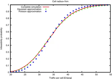
Moreover we build explicit approximate formulae for the performance eval-uation of FC load control in a hexagonal network in terms of the infeasibility probability (defined as the probability that FC doesn’t hold for a given cell when the users are modelled as a Poisson process –semi-static model).
6 CHAPTER 1. INTRODUCTION
1.3
Organization
The present part is organized as follows.
In the premilinary chapter 2 we characterize the performance of each single link, describe the model and present the notation.
In Chapter 3 we build decentralized conditions for the feasibility of the power allocation problem in a static traffic model.
In Chapter 4 we evaluate the performance of these conditions in a semi-static traffic model.
Chapter 2
Preliminaries
2.1
Single link performance
The present section is just a collection of the relevant results from the literature to which we refer the reader for more details. The multi-path fading channel may be modelled as a linear time varying Input/output model [51, Chapter 9]
vm=
L
X
k=1
gk,mum−k+ zm
where {um} is the input, {vm} is the output, {gk,m} is the channel filter and
{zm} designates the noise. The multi-path channel is characterized by the
sta-tistics of the channel filter. The noise is assumed to be additive white Gaussian (AWGN) with (power-spectral) density N0.
The multi-path fading channel may be seen as a random channel with AWGN noise as that analyzed in [31, §III.4.1]. The performance of a given
modula-tion scheme may be expressed by its bit-rate, r, and a curve giving the
error-probability as function of the energy-per-bit to noise-density ratio, Eb/N0, at
the input of the receiver. It is usual to fix some error-probability threshold, and deduce the corresponding Eb/N0 threshold. In general, we have several
modulations and a specific Eb/N0 threshold for each one.
[118, §3.4.3] studies the modulation performance in a CDMA network such as UMTS Release 99 where active users use simultaneously the entire system bandwidth. Using the arguments in [53, §6.3], [118, §3.4.3], we deduce that for this system the energy-per-bit Ebis averaged over fading.
The signal and noise powers are given respectively by S = rEb, N = W N0
where r is the bit-rate, Ebis the energy-per-bit and W is the bandwidth (5 MHz
for UMTS). Hence the signal-to-noise ratio, denoted S/N , equals S N = r W Eb N0 7
8 CHAPTER 2. PRELIMINARIES
In practice, we have for UMTS the following relation S N = r W0 Eb N0 (2.1) where W0designates the chip-rate (W0= 3.84 MHz for UMTS). For each
modu-lation, given the error-probability threshold we get the Eb/N0and S/N
thresh-olds.
We apply now the above link performance characterization to streaming and elastic traffic. A streaming call requires to transmit for some duration with a given modulation, i.e. a given bit-rate and energy-per-bit to noise-density ratio Eb/N0, and thus a given S/N threshold. It is served by a (fixed
bit-rate) Dedicated CHannel (DCH) in UMTS. If the required rate may not be offered, then the call is blocked (by the admission control scheme). We may consider different streaming classes, each characterized by a specific S/N threshold.
An elastic call has an amount of data to transmit at a bit-rate among a (fi-nite) set of possible rates which may be adjusted by the network (by the conges-tion control scheme). Elastic calls may be served by the Downlink Shared CHannel (DSCH) in UMTS. The Eb/N0thresholds of the various modulations
used on DSCH (called DSCH modulations) are close [64, §12.5.1], so we may take a single representative Eb/N0 and assume that the set of possible rates is
continuous: R+. With this assumption we get the linear relation (2.1) between
the S/N ratio and the bit-rate r.
We may also consider the Shannon’s bound which gives the theoretical
maximal bit-rate over an AWGN channel
r = W log2 µ 1 + S N ¶ (2.2) where the parameters are the same as for the previous display. For a steaming call, the bit-rate is fixed, hence we may deduce from (2.2) the corresponding S/N threshold. For an elastic call, Equation (2.2) is a non linear relation between the S/N ratio and bit-rate. Using the property of the log function we have the bound
S
N ≥
r
W ln (2) (2.3)
and, if S/N ¿ 1 then we have the approximation S
N '
r
W ln (2) (2.4)
hence we get also in this case a linear relation between the S/N ratio and the bit-rate.
Once the single link performance is characterized, we should take into ac-count the interference between the different links. To this end, we make the ap-proximation that the interference observed by some user may be approximated
2.2. MODEL 9 (averaged over the multipath fading). This approximation is justified by the large number of interferers (Central Limit Theorem) in [118, §4.3.1]. Hence the S/N threshold may be called the signal-to-interference-and-noise ratio (SINR) threshold.
2.2
Model
We now describe the considered multiple access scheme, the cell patterns (base station positions), the propagation model, the antenna types and the typical nu-merical values for UMTS system used in the nunu-merical applications throughout the present part.
2.2.1
Multiple access
In order to simplify the presentation, we focus in the present part on CDMA networks such as UMTS Release 99 (recall that in such system the active users use simultaneously the entire system bandwidth). However, our approch is sufficiently general and may be extended to wireless cellular networks with other multiple access schemes (cf., for example, Chapter 11 for TDMA and Chapter 12 for FDMA).
2.2.2
Cell pattern
The radio part of a wireless cellular network comprizes some base stations. Each base station has an antenna and serves a geographic zone called cell. The cell is defined as the set of locations in the plane which receive a signal from a base station which is stronger than the signal from any other base station. We assume in the present study that each user is served by a single base station (no macrodiversity). The effect of macrodiversity (that is a user may be served by several base stations) on the stability of a wireless cellular network serving elastic traffic is studied for example in [28].
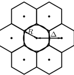
We consider a hexagonal model where the base stations are placed on a regular grid denoted on the complex plane by {∆(p + qeiπ/3); (p, q) ∈ Z2} where
∆ is the distance between two adjacent base stations and Z designates the set of all the integers, both positive and non-positive. Denote by λSthe mean number
of base stations per km2. Let R be defined by the formula
λS= 1/(πR2) (2.5)
Bearing this definition in mind, we call R the cell radius. The cell radius is in fact the radius of the disc whose area is equal to that of the hexagon. In order to simplify some calculations, we make the following approximation (as in [80]).
Approximation 1 From hexagon to disc. We approximate the hexagonal
10 CHAPTER 2. PRELIMINARIES
R ∆
Figure 2.1: Hexagon to disc approximation
Lemma 1 The cell radius R is related to the distance ∆ between two adjacent
hexagons by ∆2= 2πR2/√3, or equivalently
R = ∆
s √ 3
2π (2.6)
Numerically this gives R ' 0.525 ∆.
Proof. Let r be the radius of the circumscribed circle to a hexagon. It is easy to see that ∆ = r√3. The surface of a hexagon is 61
2r∆2 =
√
3
2 ∆2. Hence
we should have √3
2 ∆2= πR2 which gives the desired relation.
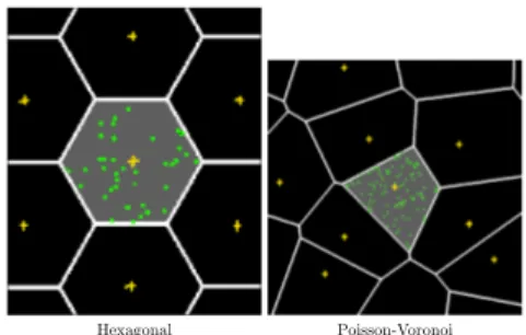
We consider sometimes a pattern where base station positions constitute a Poisson process in the plane, with intensity λS. The cell pattern in this model
is called Poisson-Voronoi. The hexagonal and Poisson-Voronoi models are illustrated in Figure 2.2. Note that the base station locations as well as the cells are random in the Poisson-Voronoi model. We always assume that the Poisson process of base stations is independent from all other considered random elements.
The hexagonal and Poisson-Voronoi models are extreme and complementary architectures: The hexagonal model represents perfectly structured networks, whereas the Poisson-Voronoi model takes into account irregularities of real net-works in a statistical way. We shall treat in details the hexagonal model and just recall the results for the Poisson-Voronoi model from [16] for the purpose of comparison.
We consider large networks where the number of base stations and the area covered by the network may be very large. We consider both the downlink (from the base stations to the users) and the uplink (from the users to the base stations).
If the network is modelled on some bounded zone of R2, then the cells at the
frontier of the zone don’t suffer the same interference as the cells in the center of the zone. In this case we model the network on a torus in order to avoid the border effect.
2.2. MODEL 11
Hexagonal Poisson-Voronoi
Figure 2.2: Hexagonal and Poisson-Voronoi models
2.2.3
Propagation
We model propagation-loss on distance r by
L (r) = (Kr)η (2.7)
where η > 2 is the so-called propagation exponent and K > 0 is a mul-tiplicative constant. The above formula represents the effect of the distance which is the principal cause of the received signal variations.
In order to simplify some formulae we introduce the normalized propagation-loss
l (r) = L (r) /L(R)
where R designates the cell radius.
The objects in the path between the antenna and the user (as for e.g. hills, buildings, trees, etc.) affect also the received signal. We may distinguish two scales of these variations: fast fading and shadowing (called also slow fading). Fast fading is related to multi-path propagation [51, Chapter 9] and induces variations over about half a wavelength. The effect of fast fading on the perfor-mance of a single link is studied in [118, §3.4.3] and recalled briefly in Section 2.1. Shadowing is related to diffraction over the obstacles in the path between the antenna and the user and induces variations over several wavelengths. Measure-ments have shown that the shadowing factor is log-normal distributed. We will not take into account the shadowing effect in the present work.
2.2.4
Antennas
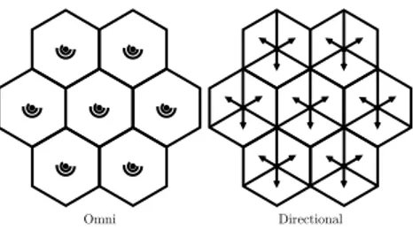
We will consider the following two versions of the hexagonal network (see Fig-ure 2.3):
• Omni: each base station is equipped with an omni antenna; this antenna
serves users in the whole disc around the base station.
• Directional: each base station is equipped with a directional antenna;
each antenna serves users in its sector defined as the set of locations in the disc within the cone of 120◦ around the antenna’s azimuth.
12 CHAPTER 2. PRELIMINARIES
Omni Directional
Figure 2.3: Illustration of the two versions of the hexagonal network: omni and directional.
In real network the power transmitted by the antennas and by the users is limited by some maximal-power constraints. We consider the cases with and without power limit. Even if the case “without power limit” isn’t realistic, we will see that it is a limit of the case “with power limit” when the cell radius is small which is the case for dense urban zones.
We denote by ˜P the maximum power including the transmitting and
re-ceiving antenna gains, denoted G, and losses, denoted L (which may include transmitting and receiving antenna loss, body loss, indoor loss, etc.). We denote
by ˆP the maximum power which doesn’t account for G and L, i.e.
ˆ
P = ˜P − G + L
2.2.5
UMTS numerical parameters
Unless otherwise specified, the following values are used for the numerical ap-plications throughout the present part.
Propagation
We consider the following propagation-loss parameters η = 3.38, K = 8667 (which correspods to the so-called Cost-Hata propagation model in an urban area [45]).
Cell radius
We consider the following cell radii
R =
½
0.525, 1, 2, . . . , 5km for the downlink 0.525, 1, 2, 3km for the uplink
2.2. MODEL 13 Antenna parameters
By default, we consider omni antennas with loss L = 0 and gain(1)
G = ½
9dBi for the downlink 12dBi for the uplink
(The antenna gain isn’t null because the energy is focused on a plan). For directional antennas we take
G = ½
12dBi for the downlink 15dBi for the uplink
The maximum power (without antenna gain and loss) equals ˆP = 43dBm(2)
for the base stations and ˆP = 21dBm for the mobiles.
Downlink specific parameters
A supplementary limit on the power transmitted to each user is sometimes imposed, typically 36dBm (without antenna gain and loss). In the present work, we have only considered the limit on the total power transmitted by the base station.
The common channels (CCH), including pilot, synchronization and paging channels, have a constant power, denoted P0. We assume that P0 is a fraction
of the maximal power
P0= ² ˜P
where ² = P0/ ˜P = 0.12.
Orthogonality factor
The orthogonality factor, denoted α, affects the intra-cell interference. Typically
α =
½
0.4 in the downlink 1 in the uplink
The orthogonality factor takes into account approximately the loss of orthogo-nality of the spreading sequences within a cell due to the multi-path. Hence α = 0 for perfectly orthogonal. (Therefore, we should call α the non-orthogonality factor, but it is the usage to call it the orthogonality factor.)
Noise power
Typically, the noise power equals
N =
½
−103dBm in the downlink −105dBm in the uplink
1The antenna gain G is a ratio of two powers, hence it has not a unit. The logarithmic representation, 10 log10(·), may be expressed in dB, which is denoted ”dBi” in the particular case of antenna gains.
14 CHAPTER 2. PRELIMINARIES
Link \service voice data 64kbps(3) data 144kbps data 384kbps
Downlink −16 −11 −9 −5
Uplink −18 −14 −12 −8
Table 2.1: SINR thresholds in dB for UMTS vehicular-A channel. SINR thresholds
Unless otherwise specified, calculations are made for voice with SINR threshold
ξ =
½
−16dB in the downlink −18dB in the uplink
We consider sometimes other streaming classes whose SINR thresholds are given in Table 2.1 (from [81]).
Eb/N0 threshold
We take for elastic services on the DSCH in UMTS a single representative value of the Eb/N0equal to 5dB [64, §12.5.1].
2.3
Notation
We will use the following notation.
2.3.1
Antenna locations and path loss
• u, v designate indexes for base stations.
• m, n designate indexes for users (mobiles). The letter designating a base
station (or a user) is sometimes used to designate it geographic position.
• U is the set of base stations (which is assumed finite, but some results
may be extended to the infinite case [16]).
• M is the set of users.
• We denote m ∈ u to say that a user m is served by base station u. Hence
we use the same letter to designate the base station and the set of users it serves.
• Lu,m is the propagation-loss between base station u and user m. For the
propagation-loss function (2.7) we get Lu,m = L (d (u, m)) where d (u, m)
designates the Euclidian distance between a user at position m and a base station at position u.
2.3. NOTATION 15
2.3.2
Engineering parameters
• ξm is the signal-to-interference-and-noise ratio threshold for user m.
• N is the external noise power. • α is the orthogonality factor.
• In order to simplify the formulae we introduce
αuv =
½
1 if v 6= u ∈ U
α if v = u ∈ U
and the modified SINR
ξ0
m= ξm/ (1 + αξm) , m ∈ M
• In the downlink, we will use the following notation:
– ˜Pu designates the maximal total power of base station u;
– Pu,mdesignates the power of dedicated channel (DCH) of user m ∈ u;
– P0
u is the power of common channels of base station u which is a
fraction of the maximal power
P0
u= ² ˜Pu, u ∈ U
where ² is a given constant. – Pu= Pu0+
P
m∈uPu,mis the total power transmitted by base station
u.
• In the uplink, we will use the following notation:
– ˜Pmdesignates the maximum power of user m.
– Pmdesignates the power transmitted by user m.
– Iu = N +
P
v∈Uαuv
P
n∈vPv/Lu,n is the total power (sum of noise
and powers from all the users) received at base station u. We will call Iuthe total interference received at base station u.
• We shall see that the following parameter, called f-factor, plays an
important role in the analysis of the performance of cellular networks
f (m) =X
v6=u
Lu,m/Lv,m, u ∈ U
(See Annex 13.B for the properties and in particular the moments of the f-factor.)
16 CHAPTER 2. PRELIMINARIES
2.3.3
Mathematics
For a random variable Z we denote ¯Z its expectation, i.e.
¯
Z = E£Z¯¤
In particular for a function f (m) of the user m ∈ u we denote ¯
f = E [f (n)]
Chapter 3
Feasibility conditions
The objective of the present chapter is to build decentralized conditions for the feasibility of the power allocation problem in a static traffic model.
The present chapter is organized as follows. In Section 2.1 we characterize the single link performance. The following two Sections 3.1 and 3.2 correspond to the downlink and uplink respectively with similar contents.
Section 3.1 is composed of 2 subsections. In subsection 3.1.1 we state the power allocation feasibility problem which rises from the interactions between the different radio links. In subsection 3.1.2 we solve this problem by building decentralized feasibility conditions.
In Section 3.3 we describe admission control schemes based on the feasibility conditions.
3.1
Downlink
We consider here the downlink (DL), i.e. the link from the base stations to the users. The reverse or uplink (UL) is treated in the following section.
The downlink power allocation is studied in [126], [87], [112], [63] and [16]. A first difference from the uplink case is the orthogonality factor α which affects the intra-cell interference only in the downlink. Moreover in the downlink there are common channels (such as the pilot channel) which have to be taken into account as interferers. Finally, interference in the downlink comes from the base stations which have fixed locations whereas the interference in the uplink comes from the users which have variable locations. We will see that in spite of these differences, the algebras of the power allocation problems of the two links present some similarities.
The authors of [16] consider the downlink with neither power limit nor com-mon channels. We extend their results to take into account these two features. Moreover we propose explicit approximate methods to evaluate the probabil-ity that the power allocation is infeasible (for a Poisson user population and a hexagonal base station architecture).
18 CHAPTER 3. FEASIBILITY CONDITIONS
3.1.1
Power allocation problem
We aim to formulate the power allocation problem for a given base station positions and user population (fixed positions {m} and SINR thresholds {ξm}).
We will say that power allocation is feasible if there exist powers such that the SINR for each user m is larger than the SINR threshold ξm.
Proposition 1 Matrix representation. The downlink power allocation
prob-lem is feasible if there exist powers {Pu,m∈ R+; m ∈ u ∈ U} such that
Pu,m/Lu,m
N − αPu,m/Lu,m+
P
v∈UαuvPv/Lv,m
≥ ξm, m ∈ u ∈ U (3.1)
The problem above may be written
½
(1 − A) P ≥ a
P ≥ 0 (3.2)
where the matrix A= [Am,n] is given by
Am,n= αuvξm0 Lu,m/Lv,m, m ∈ u ∈ U, n ∈ v ∈ U (3.3)
the vector a = (am)T (where T designates the transpose operation) is given by
am= Ã N +X v∈U αuvPv0/Lv,m ! Lu,mξm0 , m ∈ u ∈ U
and the vector P = (Pu,m)T.
The power allocation problem above is feasible iff1
ρ (A) < 1 in which case
P∗= (1 − A)−1
a (3.4)
is the minimal solution.
Proof. The power received by user m from its serving base station u is
Pu,m/Lu,m. The interference due to another user n ∈ u is Pu,n/Lu,m. Then the
interference due to own cell, called intra-cell interference, is
Iu,m(i) = α P0 u+ X n∈u\{m} Pu,n
/Lu,m= α (Pu− Pu,m) /Lu,m, m ∈ u
The interference due to other cells, called inter-cell interference, is
I(e)
u,m=
X
v∈U\{u}
Pv/Lv,m, m ∈ u
3.1. DOWNLINK 19 Hence, the signal-to-interference-and-noise ratio equals
Pu,m/Lu,m
N + α (Pu− Pu,m) /Lu,m+
P
v∈U\{u}Pv/Lv,m
which may be rearranged to get the left hand side of the inequality (3.1). (When we neglect the noise term N = 0, Inequality (3.1) is similar to [126, Equation (3) and Definition §III]. The inequality (3.1) is slightly different from that given in [63] because we neglect here the synchronization channel specificity considered there.)
We rearrange the inequality (3.1) as follows
Pu,m/Lu,m N +Pv∈UαuvPv/Lv,m ≥ ξ 0 m Hence Pu,m/Lu,m N +Pv∈UαuvPv0/Lv,m+ P v∈U P n∈vαuvPv,n/Lv,m ≥ ξ0 m
Then it is easy to see that Problem (3.1) may be written in the form (3.2). Corollary 12 gives the last part of the proposition.
Corollary 1 Achievable SINR targets. Assume that the ξm are constant,
i.e. ξm = ξ. We say that some SINR target is achievable if the power
allocation problem for that value of SINR is feasible. The set of achievable SINR targets is
0 ≤ ξ < 1
ρ (A0) − α
where the matrix A0=£A0
m,n
¤
is given by
A0
m,n= αuvLu,m/Lv,m, m ∈ u ∈ U, n ∈ v ∈ U
Proof. We may write A = ξ0A0. By Proposition 8, the power allocation
problem is feasible iff
ξ0ρ (A0) < 1 Note that A0
m,m = α then ρ (A0) ≥
P
n∈MA0m,n> α. Since ξ0 = ξ/ (1 + αξ),
we get the desired result. (The author [126] gives a similar result.)
Reduced problem. We aim to formulate the power allocation problem in terms of the powers {Pu; u ∈ U} transmitted by the base stations. To this end
we rearrange the inequality (3.1) as follows
Pu,m≥ Ã N +X v∈U αuvPv/Lv,m ! Lu,mξm0 , m ∈ u ∈ U
20 CHAPTER 3. FEASIBILITY CONDITIONS
We now add over the set {m ∈ u} X m∈u Pu,m≥ X m∈u à N +X v∈U αuvPv/Lv,m ! Lu,mξm0 , u ∈ U
The left term equals Pu− Pu0.
We say that the reduced power allocation problem is feasible if there exist powers {Pu∈ R+; u ∈ U} of the base stations such that
Pu≥ N X m∈u Lu,mξ0m+ Pu0 + X v∈U αuv X m∈u Lu,m/Lv,mξm0 Pv, u ∈ U (3.5)
Proposition 2 Matrix representation of the reduced problem. The
power allocation problem (3.5) may be written
½ (1 − A) P ≥ a P ≥ 0 (3.6) where Auv = αuv X m∈u Lu,m/Lv,mξ0m, u, v ∈ U (3.7) au= Pu0 + N X m∈u Lu,mξm0 , u ∈ U (3.8) and A = [Auv], a = [au] and P = (Pu)T.
The power allocation problem above is feasible iff
ρ (A) < 1 (3.9)
in which case
P∗= (1 − A)−1a (3.10)
is the minimal solution.
The condition (3.9) is a necessary and sufficient feasibility condi-tion (abbreviated by NSFC).
Proof. The first part of the proposition is just a matrix representation. (The idea of this ”reduced problem” is from [16] and we just extend it to account for the effect of common channels.)
Corollary 12 gives the last part of the proposition. Original versus reduced problem.
Proposition 3 The power allocation problem (3.2) is feasible iff the reduced
problem (3.6) is feasible. In this case their respective minimal solutions P∗ and
P∗ are related by P∗ u = Pu0 + X m∈u P∗ u,m, u ∈ U (3.11)
3.1. DOWNLINK 21 and P∗ u,m= Ã N +X v∈U αuvPv∗/Lv,m ! Lu,mξm0 , m ∈ u ∈ U (3.12)
Proof. (i) Suppose that Problem (3.2) is feasible and let P∗ = (1 − A)−1
a be the minimal solution. Let P∗= {P∗
u; u ∈ U} be defined by (3.11). From the
fact that (1 − A) P∗ = a which may be written P∗ = a + AP∗, we get (3.12).
Adding the equalities (3.12) over the set {m ∈ u}, we get X m∈u P∗ u,m= X m∈u à N +X v∈U αuvPv∗/Lv,m ! Lu,mξm0 , u ∈ U (3.13)
The left term equals P∗
u−Pu0. Then P∗is a solution of the reduced problem (3.6).
It is easy to see that in fact it is the minimal one.
(ii) Suppose now that the reduced problem (3.6) is feasible and let P∗ =
(1 − A)−1a be the minimal solution. Let P∗=©P∗
u,m; m ∈ u ∈ U
ª
be defined by (3.12). Adding the equalities (3.12) over the set {m ∈ u}, we get (3.13). Observe that the right-hand side of (3.13) equals P∗
u − Pu0 since P∗ satisfies
P∗ = a + AP∗. Hence we get P
m∈uPu,m∗ = Pu∗ − Pu0. Replacing Pv∗ by
P0
v+
P
n∈vPv,n∗ in the right-hand side of (3.12) shows that P∗ is the minimal
solution of Problem (3.2). (Note that [16] defines a local and a global problem and shows that the power allocation feasibility is equivalent to the feasibility of both the local and global problems. We show in Proposition 3 that there is no need to introduce the local problem.)
The above proposition shows that the condition for the feasibility of the reduced problem should be the same as that for the original problem. Therefore
ρ (A) < 1 ⇔ ρ (A) < 1
In fact we have the following stronger result. Proposition 4 We have
σ (A) \ {0} = σ (A) \ {0}
where σ (A) and σ (A) designate the sets of eigenvalues of A and A respectively; and in particular
ρ (A) = ρ (A)
Proof. From Equation (3.3) we deduce that AT
m,n= αvuLv,n/Lu,nξn0, m ∈ u, n ∈ v
We know that A and AT have the same eigenvalues. Consider a eigenvector x
of AT corresponding to a non zero eigenvalue λ. Then
X v∈U αvu X n∈v Lv,n/Lu,nξ0nxn= λxm, m ∈ u
22 CHAPTER 3. FEASIBILITY CONDITIONS
So xm depends only on the base station u serving the user m. Denote the
common value xu. Then
X v∈U αvu X n∈v Lv,n/Lu,nξn0xv= λxu
Recall that is given by (3.7), then the above equation may be written X
v∈U
Avuxv = λxu
Hence ATx = λx, which means that x = (x
u)T is an eigenvector of AT
corre-sponding to the eigenvalue λ.
Inversely from an eigenvector x = (xu)T of AT corresponding to a non zero
eigenvalue λ we construct a vector x= (xm)T by xm= xu. It is easy to see that
x is an eigenvector of AT corresponding to the eigenvalue λ.
Then ATand AT have the same non zero eigenvalues. We deduce that A and
A have the same non zero eigenvalues.
Power limitation. In the case where there is a power limitation constraint, the power allocation problem becomes
½ (1 − A) P ≥ a 0 ≤ P ≤ ˜P (3.14) where ˜P = ³ ˜ Pu ´T
designates the vector of the base station power limits. Proposition 5 The power allocation problem above is feasible iff
ρ (A) < 1 and (1 − A)−1a ≤ ˜P (3.15)
In this case, the minimal solution is P∗= (1 − A)−1
a.
The condition (3.15) is a necessary and sufficient feasibility condi-tion (abbreviated by NSFC).
Proof. Immediate from Proposition 2.
3.1.2
Feasibility conditions
Without power limit. We use the fact that the spectral radius of a matrix is lower than the maximum row sum [85, Exercice 8.2.7] to establish a sufficient condition for the feasibility of the power allocation problem (3.6).
Proposition 6 If X m∈u ξ0 m X v∈U αuvLu,m/Lv,m< 1, u ∈ U (3.16)
3.1. DOWNLINK 23 The inequality in the above proposition is called downlink feasibility condition abbreviated by DFC (or simply FC when there is no need to precise “for the downlink without power limit”).
Proof. The row sums of A may be written as follows X v∈U Auv= X m∈u ξ0 m X v∈U αuvLu,m/Lv,m, u ∈ U
The spectral radius ρ (A) is less than the largest row sum of A which is less than 1 under DFC. Then DFC implies ρ (A) < 1 which implies that power allocation problem is feasible by Proposition 2. (The idea of this sufficient feasibility condition is from [16].)
With power limit. We shall now establish a sufficient condition for the fea-sibility of the power allocation problem with power limit.
Proposition 7 If
(1 − A) ˜P ≥ a (3.17)
then the power allocation problem (3.14) is feasible and admits P∗= (1 − A)−1
a as the minimal solution. The above inequality is equivalent to
X m∈u ξ0 mLu,m à X v∈U αuvP˜v/Lv,m+ N ! ≤ ˜Pu− Pu0, u ∈ U (3.18)
The inequality in the proposition above which is called extended down-link feasibility condition, abbreviated by EDFC or simply FC when there is no need to precise “for the downlink with power limit”.
Proof. Since the vector ˜P is non-negative and satisfies (3.17) we deduce that
ρ (A) < 1 and hence (1 − A)−1is non-negative. Then ˜P = (1 − A)−1(1 − A) ˜P ≥
(1 − A)−1a. Hence (3.15) is satisfied which finishes the first claim of the
propo-sition.
Condition (3.17) may be written as follows
au≤ Ã ˜ Pu− X v∈U AuvP˜v ! , u ∈ U
which is equivalent to EDFC.
In the case where ˜Pu= ˜P is the same for all base stations, EDFC becomes
X m∈u à X v∈U αuvLu,m/Lv,m+ N Lu,m/ ˜P ! ξ0 m≤ 1 − Pu0/ ˜P , u ∈ U (3.19) If ˜P → ∞ we find X m∈u X v∈U αuvLu,m/Lv,mξm0 ≤ 1, u ∈ U