HAL Id: hal-00272432
https://hal.archives-ouvertes.fr/hal-00272432
Submitted on 11 Apr 2008
HAL is a multi-disciplinary open access
archive for the deposit and dissemination of
sci-entific research documents, whether they are
pub-lished or not. The documents may come from
teaching and research institutions in France or
abroad, or from public or private research centers.
L’archive ouverte pluridisciplinaire HAL, est
destinée au dépôt et à la diffusion de documents
scientifiques de niveau recherche, publiés ou non,
émanant des établissements d’enseignement et de
recherche français ou étrangers, des laboratoires
publics ou privés.
Medial Axis LUT Computation for Chamfer Norms
Using H-Polytopes
Nicolas Normand, Pierre Évenou
To cite this version:
Nicolas Normand, Pierre Évenou. Medial Axis LUT Computation for Chamfer Norms Using
H-Polytopes.
Discrete Geometry for Computer Imagery, Apr 2008, Lyon, France.
pp.189-200,
�10.1007/978-3-540-79126-3_18�. �hal-00272432�
Medial Axis LUT Computation for Chamfer Norms Using H-Polytopes
Nicolas Normand, Pierre ´Evenou
IRCCyN/IVC UMR CNRS 6597
Abstract. Chamfer distances are discrete distances based on the propagation of local distances, or
weights defined in a mask. The medial axis, i.e. the centers of the maximal disks (disks which are not contained in any other disk), is a powerful tool for shape representation and analysis. The extraction of maximal disks is performed in the general case with comparison tests involving look-up tables rep-resenting the covering relation of disks in a local neighborhood. Although look-up table values can be computed efficiently, the computation of the look-up table neighborhood tend to be very time-consuming. By using polytope descriptions of the chamfer disks, the necessary operations to extract the look-up tables are greatly reduced.
@inproceedings{normand2008dgci,
Title = {Medial Axis {LUT} Computation for Chamfer Norms Using {H}-Polytopes}, Author = {Normand, Nicolas and {\’E}venou, Pierre},
Booktitle = {Discrete Geometry for Computer Imagery},
Editor = {Coeurjolly, David and Sivignon, Isabelle and Tougne, Laure and Dupont, Florent}, Doi = {10.1007/978-3-540-79126-3_18},
Keywords = {Discrete distance, chamfer distance, weighted distance, polytope, medial axis}, Month = apr,
Pages = {189-200},
Publisher = {Springer Berlin / Heidelberg}, Series = {Lecture Notes in Computer Science}, Volume = {4992},
Year = {2008}}
Medial Axis LUT Computation for Chamfer
Norms Using
H-Polytopes
Nicolas Normand and Pierre ´Evenou [email protected]
IRCCyN UMR CNRS 6597, ´Ecole polytechnique de l’Universit´e de Nantes, Rue Christian Pauc, La Chantrerie,
44306 Nantes Cedex 3, FRANCE.
Abstract. Chamfer distances are discrete distances based on the prop-agation of local distances, or weights defined in a mask. The medial axis,
i.e. the centers of the maximal disks (disks which are not contained in
any other disk), is a powerful tool for shape representation and analysis. The extraction of maximal disks is performed in the general case with comparison tests involving look-up tables representing the covering re-lation of disks in a local neighborhood. Although look-up table values can be computed efficiently [1], the computation of the look-up table neighborhood tend to be very time-consuming. By using polytope [2] de-scriptions of the chamfer disks, the necessary operations to extract the look-up tables are greatly reduced.
1
Introduction
The distance transform DTX of a binary image X is a function that maps each
point x with its distance to the background i.e. with the radius of the largest open disk centered in x included in the image. Such a disk is said to be maximal if no other disk included in X contains it. The set of centers of maximal disks, the medial axis, is a convenient description of binary images for many applications ranging from image coding to shape recognition. Its attractive properties are reversibility and (relative) compactness.
Algorithms for computing the distance transform are known for various crete distances [3–6]. In this paper, we will focus on chamfer (or weighted) dis-tances. The classical medial axis extraction method is based on the removal of non maximal disks in the distance transform. It is thus mandatory to describe the covering relation of disks, or at least the transitive reduction of this relation. For simple distances this knowledge is summarized in a local maximum criterion [3]. The most general method for chamfer distances uses look-up tables for that purpose [7].
In this paper we propose a method to both compute the look-up tables and the look-up table mask based on geometric properties of the balls of chamfer norms. Basic notions, definitions and known results about chamfer disks and
medial axis look-up tables are recalled in section 2. Then section 3 justifies the use of polytope formalism in our context and presents the principles of the method. In section 4, algorithms for the 2D case are given.
2
Chamfer Medial Axis
2.1 Chamfer DistancesDefinition 1 (Discrete distance, metric and norm). Consider a function
d :Zn× Zn→ N and the following properties ∀x, y, z ∈ Zn, ∀λ ∈ Z:
1. positive definiteness d(x, y) ≥ 0 and d(x, y) = 0 ⇔ x = y , 2. symmetry d(x, y) = d(y, x) ,
3. triangle inequality d(x, z) ≤ d(x, y) + d(y, z) , 4. translation invariance d(x + z, y + z) = d(x, y) , 5. positive homogeneity d(λx, λy) = |λ| · d(x, y) .
d is called a distance if it verifies conditions 1 and 2, a metric with conditions
1 to 3 and a norm if it also satisfies conditions 4 and 5.
Most discrete distances are built from a definition of neighborhood and con-nected paths (path-generated distances), the distance from x to y being equal to the length of the shortest path between the two points [8]. Distance functions differ by the way path lengths are measured: as the number of displacements in the path for simple distances like d4 and d8, as a weighted sum of
displace-ments for chamfer distances [4] or by the displacedisplace-ments allowed at each step for neighborhood sequence distances [8, 4], or even by a mixed approach of weighted neighborhood sequence paths [6].
For a given distance d, the closed ball Bc and open ball Bo of center c and
radius r are the sets of points of Zn:
Bo(c, r) = {p : d(c, p) < r}
Bc(c, r) = {p : d(c, p) ≤ r} . (1)
Since the codomain of d is N: ∀r ∈ N, d(c, p) ≤ r ⇔ d(c, p) < r + 1. So:
∀r ∈ N, Bc(c, r) = Bo(c, r + 1) . (2)
In the following, the notation B will be used to refer to closed balls. Definition 2 (Chamfer mask [9]). A weighting M = (−→v ; w) is a vector −→v of Zn associated with a weight w (or local distance). A chamfer mask M is
a central-symmetric set of weightings having positive weights and non-null dis-placements, and containing at least one basis of Zn: M = {M
i∈ Zn× N∗}1≤i≤m
The grid Zn is symmetric with respect to the hyperplanes normal to the
octants for Z2). Chamfer masks are usually G-symmetric so that weightings may
only be given in the sub-space 0 ≤ xn≤ . . . ≤ x1.
Paths between two points x and y can be produced by chaining displacements. The length of a path is the sum of the weights associated with the displacements and the distance between x and y is the length of the shortest path.
Definition 3 (Chamfer distance [9]). Let M = {(−→vi, wi) ∈ Zn× N∗}1≤i≤m
be a chamfer mask. The chamfer (or weighted) distance between two points x and y is: d(x, y) = min!"λiwi: x + " λi−→vi = y, λi ∈ N, 1 ≤ i ≤ m # . (3)
Any chamfer masks define a metric [10]. However a chamfer mask only generates a norm when some conditions on the mask neighbors and on the corresponding weights permits a triangulation of the ball in influence cones [9, 11]. When a mask defines a norm then all its balls are convex.
2.2 Geometry of the Chamfer Ball
We can deduce from (1) and (3) a recursive construction of chamfer balls:
B(O, r) = B(O, r− 1) ∪ $
0≤i≤m
B(O + −→vi, r− wi) . (4)
Definition 4 (Influence cone [12]). Let M = {(−→vi, wi) ∈ Zn× N∗}1≤i≤m
be a chamfer mask generating a norm. An influence cone is a cone from the origin spanned by a subset of the mask vectors {−→vi, −→vj, −→vk, . . .} in which only the
weightings Mi, Mj, Mk, . . . of the mask are involved in the computation of the
distance from O to any point of the cone.
In each influence cone, the discrete gradient of the distance function is constant and equal to [9]:
(wi, wj, wk, . . .)· (−→vi|−→vj|−→vk| . . .)−1 , (5)
where (−→vi|−→vj|−→vk| . . .) stands for the column matrix of the vectors spanning the
cone. The distance dC(O, p) from the origin to any point p of this cone C is then:
dC(O, p) = (wi, wj, wk, . . .)·% −→vi −→vj −→vk. . .&−1· p . (6)
For instance, with chamfer norm d5,7,11, the point (3, 1) is in the cone spanned
by the vectors a = (1, 0) and c = (2, 1) and the weights involved are 5 and 11. The distance between the origin and the point (3, 1) is then:
dCa,c(O, (3, 1)) = %5 11& · '1 2 0 1 (−1 · '3 1 ( =%5 1&·'31(= 16 .
2.3 Chamfer Medial Axis
For simple distances d4 and d8, the medial axis extraction can be performed
by the detection of local maxima in the distance map [13]. Chamfer distances raise a first complication even for small masks as soon as the weights are not unitary. Since all possible values of distance are not achievable, two different radii r and r$may correspond to the same set of discrete points. The radii r and
r$ are said to be equivalent. Since the distance transform labels pixels with the
greatest equivalent radius, criterions based on radius difference fail to recognize equivalent disks as being covered by other disks. In the case of 3 × 3 2D masks or 3 × 3 × 3 3D masks, a simple relabeling of distance map values with the smallest equivalent radius is sufficient [14, 15]. However this method fails for greater masks and the most general method for medial axis extraction from the distance map involves look-up tables (LUT) that represent for each radius r and displacement −→vi, the minimal open ball covering Bo(O, r1,) in direction −→vi [7]:
Lut−→vi(r1) = min{r2: B
o(O + −→v
i, r1) ⊆ Bo(O, r2)} .
Equivalently using closed balls (considering (2)):
Lut−→vi(r1) = 1 + min{r2: B(O + −→vi, r1− 1) ⊆ B(O, r2)} . (7)
Consider for instance the d5,7,11 distance [16, Fig. 14]. Lut(1,0)(10) = 12
means that Bo(O, 10) ⊆ Bo((2, 1), 12) but Bo(O, 10) +⊆ Bo((2, 1), 11). Or, in
terms of closed balls, B(O, 9) ⊆ B((2, 1), 11) but B(O, 9) +⊆ B((2, 1), 10). Medial Axis LUT Coefficients. A general method for LUT coefficient com-putation was given by R´emy and Thiel [12, 17, 9]. The idea is that the disk covering relation can be extracted directly from values of distance to the origin. If d(O, p) = r1 and d(O, p + −→vi) = r2, we can deduce the following:
p∈ B(O, r1) = Bo(O, r1+ 1) ,
p + −→vi ∈ B(O, r/ 2− 1) = Bo(O, r2) ,
hence Bo(O + −→v
i, r1+ 1) +⊂ Bo(O, r2) and Lut−→vi(r1+ 1) > r2. If ∀p, d(O, p) ≤
r1⇒ d(O, p + −→vi) ≤ r2 then Lut−→vi(r1+ 1) = r2+ 1.
Finally: Lut−→vi(r) = 1 + max(d(O, p + −→vi) : d(O, p) < r).
This method only requires one scan of the distance function for each dis-placement −→vi. Moreover, the visited area may be restricted according to the
symmetries of the chamfer mask. The order of complexity is about O(mLn) if
we limit the computation of the distance function to a Ln image.
Medial Axis LUT Mask. Thiel observed that the chamfer mask is not ad-equate to compute the LUT and introduced a LUT Mask MLut(R) for that
purpose [12, p. 81]. MLut(R) is the minimal test neighbourhood sufficient to
ball) is less than or equal to R. For instance, with d14,20,31,44: Lut(2,1)(291) =
321 and Lut(2,1)(321) = 352 but the smallest open ball of center O covering
Bo((4, 2), 291) is Bo(O, 351). In this particular case, the point (4, 2) is not in the
chamfer mask but should be in MLut(R) for R greater than 350.
A mask incompleteness produces extra points in the medial axis (undetected ball coverings). A general method for both detecting and validating MLut is
based on the computation of the medial axis of all disks. When MLutis complete,
the medial axis is restricted to the center of the disk, when extra points remains, they are added to MLut. This neighborhood determination was proven to work in
any dimension n ≥ 2. However it is time consuming even when taking advantage of the mask symmetries.
3
Method Basics
3.1 General H-Polytopes [2]
Definition 5 (Polyhedron). A convex polyhedron is the intersection of a finite
set of half-hyperplanes.
Definition 6 (Polytope). A polytope is the convex hull of a finite set of points. Theorem 1 (Weyl-Minkowski). A subset of Euclidean space is a polytope if
and only if it is a bounded convex polyhedron.
As a result, a polytope in Rn can be represented either as the convex hull of
its k vertices (V-description): P = conv({pi}1≤i≤k) or by a set of l half-planes
(H-description):
P ={x : Ax ≤ y} , (8)
where A is a l × n matrix, y a vector of n values that we name H-coefficients of
P . Having two vectors −→u and −→v , we denote −→u ≤ −→v if and only if∀i, −→ui≤ −→vi.
Definition 7 (Discrete polytope). A discret polytope is the intersection of a
polytope with Zn.
Minimal Representation. Many operations on Rnpolytopes in either V or H
representation often require a minimal representation. The redundancy removal is the removing of unnecessary vertices or inequalities in polytopes. Since our purpose is mainly to compare H-polytopes defined with the same matrix A, no inequality removal is needed. However, for some operations, H-representations of discrete polytopes must be minimal in terms of H-coefficients.
Definition 8 (Minimal parameter representation). We call minimal
pa-rameter H-representation of a discrete polytope P , denoted )H-representation, a H-representation P = {x : Ax ≤ y} such that y is minimal:
P ={x ∈ Zn : Ax ≤ y} and ∀i ∈ [1..l], ∃x ∈ Zn: Aix = yi , (9)
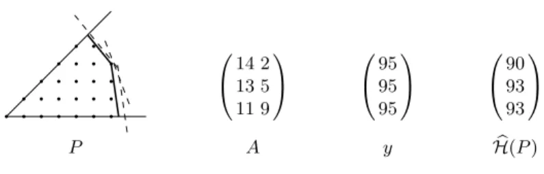
0 @14 213 5 11 9 1 A 0 @9595 95 1 A 0 @9093 93 1 A P A y H(P )b
Fig. 1. H-representations of a discrete G-symmetrical polytope P (restricted to the first octant). Dashed lines: H-representation of P . Thick lines: bH-representation of
P . In the bH case, the three equalities are verified for the same point (6, 3). Notice
that although coefficient values are minimal, this representation is still redundant: the second inequality could be removed.
The )H function which gives the minimal parameters for a given polytope P is introduced for convenience: )H(P ) = max{Ax : x ∈ P }. {x : Ax ≤ )H(P )} is the )H-representation of P = {x : Ax ≤ y}. Figure 1 depicts two representations of the same polytope P in Z2.
H-Polytope Translation. Let P = {x : Ax ≤ y} be a H-polytope. The
translated of P by −→v which is also the Minkowski sum of P and{−→v} is:
(P )−→v = P ⊕ {−→v} = {x + −→v : Ax≤ y} = {x : Ax ≤ y + A−→v} . (10)
The translation of a minimal representation gives a minimal representation.
Covering Test. Let P = {x : Ax ≤ y} and Q = {x : Ax ≤ z} be two polyhedrons represented by the same matrix A but different sets of H-coefficients
y and z. P is a subset of Q if (sufficient condition):
y≤ z ⇒ P ⊆ Q . (11)
Furthermore, if the H-description of the enclosed polyhedron has minimal coef-ficients, the condition is also necessary:
y = )H(P ) ≤ z ⇔ P ⊆ Q . (12)
3.2 Chamfer H-Polytopes
Describing balls of chamfer norms as polygons in 2D and polyhedra in higher dimensions is not new [10]. Thiel and others have extensively studied chamfer ball geometry from this point of view [12, 11, 18]. Our purpose is to introduce properties specific to the H-representation of these convex balls.
Proposition 1 (Direct distance formulation).
d(O, x) = max
1≤i≤l(dCi(x)) (13)
where l is the number of cones, dCi is the distance function in the i
thcone. Note
Proof. Equation (6) states that for all the influence cones C that contain p, dC(O, p) = d(O, p). For other cones, this relation does not hold, but it is still
possible to compute dC(O, p). The influence cone C corresponds to a facet of
the unitary real ball supported by the hyperplane {x ∈ Rn : d
C(x) = 1}. Due
to convexity, the unitary ball is included in the halfspace {x ∈ Rn : d
C(x) ≤ 1}.
This applies to the vertices of the unitary ball −→vi wi: dC(
− →vi
wi) ≤ 1. By linearity of
dC, dC(−→vi) ≤ wi and dC(*iλi−→vi) = *iλidC(−→vi) ≤ *iλiwi. dC(*iλi−→vi) is
always less than or equal to the length of the path *iλi−→vi.
Chamfer Balls H-Representation. The H-representation of chamfer balls is directly derived from (13):
x∈ B(O, r) ⇔ max
1≤i≤l{dCi(x)} ≤ r ⇔ AM· x ≤ y (14)
where AMis a H-representation matrix depending only on the chamfer mask M.
The number of rows in AMis equal to the number l of influence cones, each line
of the matrix AM is computed with (5) and y is a column vector whose values
are r. For instance, the H-representation matrix for d5,7,11 is AM =
'5 1 4 3
(
where (5 1) and (4 3) are the distance gradients in the two cones and B(O, r) = + x∈ Zn: '4 3 5 1 ( · x ≤ ' r r (, .
Proposition 2 (Furthest point). Let AMbe the matrix defined by the
cham-fer mask M generating a norm. The furthest point from the origin in the ) H-polytope P = {x : AM· x ≤ y} is at a distance equal to the greatest component
of y.
Proof. By construction of AM, (13) is equivalent to d(O, x) = maxi{AMi· x}.
max
x∈P{d(O, x)} = maxx∈P{ max1≤i≤l{AMi· x}} = max{ )Hi(P )}
Proposition 3 (Minimal covering ball). The radius of the minimal ball
cen-tered in O that contains all points of a discrete )H-polytope P represented by the matrix AM and the vector y is equal to the greatest component of y.
Proof. The smallest ball that covers the polytope P must cover its furthest point
from the origin.
min{r ∈ N : P ⊆ B(O, r)} = max
x∈P{d(O, x)} (15)
Note that if P is not centered in O, the simplification due to symmetries do not hold and the full set of H-coefficients is needed, unless we ensure that the
coefficents for the hyperplanes in the working sub-space are greater than
H-coefficients for the corresponding symmetric cones. This is the case when a G-symmetric polytope is translated by a vector in the sub-space.
Definition 9 (Covering function). We call covering function of a set X of
points of Zn the function C
X which assigns to each point p of Zn, the radius of
the minimal ball centered in p covering X: CX: 2Z
n
× Zn
→ N
X , p → min{r : X ⊆ B(p, r)} .
The covering function of the chamfer ball B(O, r) at point p gives the radius of the minimal ball centered in p that contains B(O, r). It is equal using central symmetry to the minimal ball centered in O covering B(p, r) and therefore it is the maximal component of the )H-representation of B(p, r):
CB(O,r)(p) = max{ )H(B(p, r)} = max{ )H(B(O, r)) + AM· p} . (16)
One can notice that the covering function of the zero radius disk is equal to the distance function, as is the distance transform of the complement of this disk:
CB(O,0)(p) = DTZn\{O}(p) = d(p, O) = d(O, p) .
Definition 10 (Covering cone). A covering cone Co,U in CX is a cone defined
by a vertex o and a subset U of the chamfer mask neighbor set with det(U) = ±1, Co,U= {o +*λi−→ui, λi ∈ N, −→ui ∈ U}, such that:
∀p ∈ Co,U,∀−→u ∈ U, B(p, CX(p)) ! B(p + −→u ,CX(p + −→u )) .
Proposition 4. If Co,U is a covering cone in CB(O,r) then for any point q in
Co,U\ U \ {o} there exists p such that:
B(O, r)! B(p, CB(O,r)(p)) ! B(q, CB(O,r)(q)) .
Proof. Since q += o, there always exists another point p in Co,U, distinct from q,
such that B(p, CB(O,r)(p)) ! B(q, CB(O,r)(q)). B(O, r) ⊆ B(p, CB(O,r)(p)) always
holds by definition of CB(O,r). A sufficient condition for B(O, r) += B(p, CB(O,r))
is that a point p distinct from O exists in Co,U which is always the case if q is
not equal to one of the generating vectors of Co,U.
Proposition 5. If there is a integer j ∈ [1 . . . l] and a point o such that AMj·
−
→ui,∀−→ui ∈ U and )Hj(B(o, r)) are maximal then Co,Uis a covering cone in CB(O,r).
Proof. Let j be the row number of a maximal component of )H(B(o, r)) and AM· −→ui,∀−→ui ∈ U, then j is a maximal component of any positive linear
combi-nation of these vectors. Let p be any point in Co,U, p = o + *iλi−→ui, λi ∈ N
and Bpthe minimal ball covering B(O, r). From (16) we deduce that CB(O,r) is
affine in Co,U: CB(O,r)(p) = max ! ) H (B(o, r)) +"λiAM−→ui # = )Hj(B(o, r)) + " λiAMj−→ui .
In the same way, the radius of the minimal ball centered in p + −→u , −→u ∈ U
covering B(O, r) is:
CB(O,r)(p + −→u ) = )Hj(B(o, r)) +
"
λiAMj−→ui+ AMj−→u
= CB(p,CB(O,r)(p))(O + −→u ) .
In other words, B(p, CB(O,r)(p)) is a subset of B(p + −→u ,CB(O,r)(p + −→u )).
4
LUT and
M
LutComputation for 2D chamfer norms
LUT and MLutcomputation methods for 2D chamfer norms are presented here.
Both are based on the minimal )H-representation of the chamfer balls, from which we compute the covering function and deduce the LUT values. M vectors are ordered by angle so that each influence cone is defined by two successive angles (O, {−→vi, −−→vi+1}).
4.1 H-Representation of Chamfer Balls)
The computation of the LUT is based on a )H-representation of the chamfer norm balls. All share the same matrix AM which depends only on the chamfer mask (14). )H-coefficients of balls are computed iteratively from the ball of radius 0,
B(O, 0) ={x : AMx = 0} using (4) and (10).
)
H(B(O, r)) = max{ )H(B(O, r − 1)),
)
H(B(O, r − w1)) + AM−→v1, . . . , )H(B(O, r − wm)) + AM−→vm} .
Each LUT value is obtained from the covering function (16):
Lut−→vi[r] = 1 + CB(O,r−1)(O + −→vi) = 1 + max( )H(B(O, r − 1)) + AM· −→vi) .
4.2 LUT Mask
The algorithm starts with an empty mask and balls with increasing radii are tested for direct covering relations as in [1]. However, in our case, the covering relations are seen from the perspective of the covered balls (in the covering func-tion) whereas in [1], they are considered from the point of view of the covering balls (in the distance map). Another difference lies in the computation of cov-ering radii which does not require the propagation of weights thanks to a direct formula (16). In order to remove useless points, all known LUT neighborhoods are checked for an indirect covering by the procedure visitPoint.
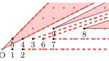
In each influence cone (O, {−→vi, −−→vi+1}), a set of covering cones are detected to
limit the search space: a 2D covering cone ((a, a), {(1, 0), (0, 1)}) with a vertex chosen on the cone bissector [O, (1, 1)), then 1D covering cones ((b, α), {(1, 0)}), ((α, b), {(0, 1)}) for α varying from 1 to a−1 (coordinates relative to (O, {−→vi, −−→vi+1})).
Fig. 2 shows the working sub-space partitioning, covering cones and visit order of points for the chamfer norm d14,20,31,44 and the inner radius 20.
O 1 2 3 4 5 6 7 8 9
Fig. 2. 1D (dashed lines) and 2D (filled areas) covering cones and visit order of points.
Algorithm 1: Computation of the look-up table mask
Input: chamfer maskM = {(−→vi; wi)}1≤i≤m, maximal radius R
MLut← ∅;
for r← 1 to R do // current inner radius, increasing order
for i← 1 to m do // visit vector axes
visit1DCone(MLut, r, O, −→vi);
end
for i← 1 to l do // visit the interior of influence cones
a← findCoveringConeVertex(r, O + α−→vi+ α−−→vi+1, −→vi+ −−→vi+1);
for α← 1 to a − 1 do // skip the covering cone
visitPoint(MLut, r, O + α−→vi+ α−−→vi+1);
visit1DCone(MLut, r, O + α−→vi+ α−−→vi+1, −→vi);
visit1DCone(MLut, r, O + α−→vi+ α−−→vi+1, −−→vi+1);
end
visitPoint(MLut, r, a· Mi+ a· Mi+1);
end end
Procedure visit1DCone(MLut, r, p, −→u )
Input:MLut, inner radius r, vertex and direction of the tested cone p, −→u
for α← 1 to findCoveringConeVertex(r, p, −→u ) do
visitPoint(MLut, r, β· Mi+ α· Mi+1);
end
Procedure visitPoint(MLut, r, p)
Input:MLut, inner radius r, ball center p to test
if ∀−→v ∈ MLut: B(O + −→v ,CB(O,r)(O + −→v ))'⊂ B(p, CB(O,r)(p)) then
MLut← MLut∪ M
end
Function findCoveringConeVertex(r, p, −→u )
Input: inner radius r, vertex and direction of the searched cone p, −→u
Output: Integer
y = bH(B(p, r)); z = AM· −→u ;
i0← argmaxi{yi: zi= max{z}} // component i0 is maximal. . .
return a = maxnlyi−yi0 zi0−zi
mo
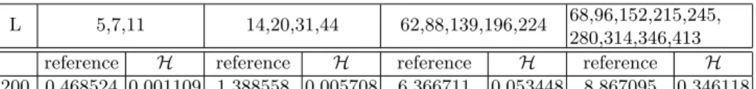
Table 1. Run times (in seconds)
L 5,7,11 14,20,31,44 62,88,139,196,224 68,96,152,215,245,
280,314,346,413
reference H reference H reference H reference H
200 0.468524 0.001109 1.388558 0.005708 6.366711 0.053448 8.867095 0.346118 500 8.315003 0.002784 25.262300 0.017302 125.293637 0.145683 177.506492 0.975298 1000 90.670806 0.007007 268.807796 0.036611 1267.910045 0.276737 1684.583989 1.778505
4.3 Results
An implementation of these algorithms was developed in C language. It produces output in the same format as the reference algorithm [16] so that outputs can be compared character-to-character. Tests were done on various chamfer masks and different maximal radii. The results are almost always identical except for insignificant cases close to the maximal radius for which covering radii exceed the maximum. Other differences may occur in the order weightings are added to
MLut(sorted with respect to the covered radius or to the covering radius).
The run times of both reference and proposed algorithms are given in Table 1 for various sizes an distances.
5
Conclusion and Future Works
In this paper methods to compute both the chamfer LUT and chamfer LUT mask were presented. Speed gains from the reference algorithm [1] are attributable to the representation of chamfer balls as H-polytopes. This description allows to avoid the use of weight propagation in the image domain and permits a constant time covering test by the direct computation of covering radii. Although not thoroughly tested, we think that LUT value computation is faster with our method due to the smaller size of the test space (linear with the radius of the maximal ball). For MLut determination, results show must faster computation
especially for large radii. This is due to the reduced search space eliminating covering cones and the constant time covering test.
While applications always using the same mask can use precomputed MLut
and LUT, other applications that potentially use several masks, adaptive masks, variable input image size can benefit from these algorithms. A faster computation of MLut is also highly interesting to explore chamfer mask properties. Beyond
improved run times, the H-polytope representation helped to prove new prop-erties of chamfer masks. And a new formula of distance which doesn’t need to find in which cone lies a point was given.
Whereas the underlying theory (H-representation of balls, translation, cov-ering test and covcov-ering cone) does not depend on the dimension, the algorithms were given only for dimension 2. In the 2D case, vectors can be ordered by an-gle so two consecutive vectors define a cone. Higher dimensions require a Farey triangulation of chamfer balls.
A paper will greater details and results is being prepared for presentation in a journal. The source code for algorithms presented here is available from the IAPR technical committee on discrete geometry (TC18)1.
References
1. R´emy, ´E., Thiel, ´E.: Medial axis for chamfer distances: computing look-up tables and neighbourhoods in 2d or 3d. Pattern Recognition Letters 23(6) (2002) 649–661 2. Ziegler, G.M.: Lectures on Polytopes (Graduate Texts in Mathematics). Springer
(2001)
3. Rosenfeld, A., Pfaltz, J.L.: Sequential operations in digital picture processing. Journal of the ACM 13(4) (1966) 471–494
4. Borgefors, G.: Distance transformations in arbitrary dimensions. Computer Vision, Graphics, and Image Processing 27(3) (1984) 321–345
5. Coeurjolly, D., Montanvert, A.: Optimal separable algorithms to compute the reverse euclidean distance transformation and discrete medial axis in arbitrary dimension. IEEE Transactions on Pattern Analysis and Machine Intelligence 29(3) (2007) 437–448
6. Strand, R.: Weighted distances based on neighborhood sequences. Pattern Recog-nition Letters (28) (2007) 2029–2036
7. Borgefors, G.: Centres of maximal discs in the 5-7-11 distance transforms. In: Proc. 8th Scandinavian Conf. on Image Analysis, Tromsø, Norway (1993) 8. Rosenfeld, A., Pfaltz, J.: Distances functions on digital pictures. Pattern
Recog-nition Letters 1(1) (1968) 33–61
9. Thiel, ´E.: G´eom´etrie des distances de chanfrein. m´emoire d’habilitation `a diriger des recherches (2001) http://www.lif-sud.univ-mrs.fr/~thiel/hdr/ .
10. Verwer, B.J.H.: Local distances for distance transformations in two and three dimensions. Pattern Recognition Letters 12(11) (1991) 671–682
11. R´emy, ´E.: Normes de chanfrein et axe m´edian dans le volume discret. Th`ese de doctorat, Universit´e de la M´editerran´ee (2001)
12. Thiel, ´E.: Les distances de chanfrein en analyse d’images : fondements et ap-plications. Th`ese de doctorat, Universit´e Joseph Fourier, Grenoble 1 (1994) http://www.lif-sud.univ-mrs.fr/~thiel/these/ .
13. Pfaltz, J.L., Rosenfeld, A.: Computer representation of planar regions by their skeletons. Communications of the ACM 10(2) (1967) 119–122
14. Arcelli, C., Sanniti di Baja, G.: Finding local maxima in a pseudo-Euclidian dis-tance transform. Computer Vision, Graphics, and Image Processing 43(3) (1988) 361–367
15. Svensson, S., Borgefors, G.: Digital distance transforms in 3d images using infor-mation from neighbourhoods up to 5×5×5. Computer Vision and Image Under-standing 88(1) (2002) 24–53
16. R´emy, ´E., Thiel, ´E.: Medial axis for chamfer distances: computing look-up tables and neighbourhoods in 2d or 3d. Pattern Recognition Letters 23(6) (2002) 649–661 17. R´emy, ´E., Thiel, ´E.: Computing 3D medial axis for chamfer distances. In: Discrete Geometry for Computer Imagery. Volume 1953., Uppsala, Sweden (2000) 418–430 18. Borgefors, G.: Weighted digital distance transforms in four dimensions. Discrete
Applied Mathematics 125(1) (2003) 161–176