Accuracy Analysis of 3T1R Fully-Parallel Robots

HAL Id: hal-00460001

https://hal.archives-ouvertes.fr/hal-00460001

Submitted on 25 Jun 2019

HAL is a multi-disciplinary open access

archive for the deposit and dissemination of sci-entific research documents, whether they are

pub-L’archive ouverte pluridisciplinaire HAL, est destinée au dépôt et à la diffusion de documents scientifiques de niveau recherche, publiés ou non,

Accuracy Analysis of 3T1R Fully-Parallel Robots

Sébastien Briot, Ilian Bonev

To cite this version:

Sébastien Briot, Ilian Bonev. Accuracy Analysis of 3T1R Fully-Parallel Robots. Mechanism and Machine Theory, Elsevier, 2010, 45 (5), pp.695-706. �hal-00460001�

Accuracy Analysis of 3T1R Fully-Parallel Robots

Sébastien Briot, Ilian A. Bonev

Department of Automated Manufacturing Engineering, École de technologie supérieure (ÉTS), Montreal, Canada e-mail: sebastien.briot.1@ens.etsmtl.ca, ilian.bonev@etsmtl.ca

ABSTRACT

Parallel robots with Shoenflies motions (also called 3T1R parallel robots) are increasingly being used in applications where precision is of great importance. Clearly, methods for evaluating the accuracy of these robots are therefore needed. The accuracy of well designed, manufactured, and calibrated parallel robots depends mostly on the input errors (sensor and control errors). Dexterity and other similar performance indices have often been used to evaluate indirectly the influence of input errors. However, industry needs a precise knowledge of the maximum orientation and position output errors at a given nominal configuration. An interval analysis method that can be adapted for this purpose has been proposed in the literature, but gives no kinematic insight into the problem of optimal design. In this paper, a simpler method is proposed based on a detailed error analysis of 3T1R fully-parallel robots that brings valuable understanding of the problem of error amplification.

I. INTRODUCTION

Parallel robots are increasingly being used for precision positioning, and a number of them are used as 4-degree-of-freedom (DOF) parallel robots, with three translations and one rotation (3T1R – also called SCARA type or Schoenflies motions), for positioning a body in space (mainly for pick-and-place applications). Clearly, in such industrial applications, accuracy is of great importance. Therefore, simple and fast methods for computing the accuracy of a given robot design are needed in order to use them in design optimization procedures that look for maximum accuracy.

Errors in the position and orientation of a parallel robot are due to several factors: − manufacturing errors, which can however be taken into account through calibration; − backlash, which can be eliminated through proper choice of mechanical

components (e.g., using direct drives);

− compliance, which can also be eliminated through the use of more rigid structures (though this would increase inertia and decrease operating speed);

− active-joint errors, coming from the finite resolution of the encoders, sensor errors, and control errors.

Therefore, as pointed out by Merlet [1], active-joint errors (input errors) are the most significant source of errors in a properly designed, manufactured, and calibrated parallel robot. In this paper, we address the problem of computing the accuracy of a parallel robot in the presence of active-joint errors only. In the balance of the paper, the term “accuracy” will therefore refer to the position and orientation errors of a parallel robot that is subjected to active-joint errors only.

  p J q (1) where q represents the vector of the active-joint (input) errors, p the vector of output errors and J is the Jacobian matrix of the robot. However, this method will give only an approximation of the output maximum error.

Several performance indices have been developed and used to roughly evaluate the accuracy of serial and parallel robots. A recent study [2] reviewed most of these performance indices and discussed their inconsistencies when applied to parallel robots with translational and rotational degrees of freedom. The most common performance indices used to indirectly optimize the accuracy of parallel robots are the dexterity index [3], the condition numbers [4], and the global conditioning index [5]. However, in a recent study of the accuracy of a class of 3-DOF planar parallel robots [6], it was demonstrated that dexterity has little to do with robot accuracy, as we define it.

Obviously, the best accuracy measure for an industrial parallel robot would be the maximum position and maximum orientation errors over a given portion of the workspace [1], [6]-[9] or at a given nominal configuration, given actuator inaccuracies. A general method based on interval analysis for calculating close approximations of the maximum output error over a given portion of the workspace was proposed recently in [1]. Clearly, the maximum output error over a given portion of the workspace is the most important information for a designer. However, this method is relatively difficult to implement, gives no information on the evolution of the accuracy of the manipulator within its workspace and gives no kinematic insight into the problem of optimal design. In contrast, simple geometric methods for computing the exact value of the accuracy of 2-DOF and 3-DOF planar parallel robots were described in [6]-[8] . These methods propose to replace the existing dexterity maps by maximum position error maps and maximum orientation error maps. While these methods

cover three of the most promising designs for precision parallel robots (one of which is commercialized and the other two built into laboratory prototypes), they work only for 2-DOF or 3-DOF planar parallel robots, and not for other mechanisms, such as 3T1R fully-parallel manipulators.

There are a high number of 3T1R fully-parallel architectures [10]-[19]. Therefore finding a general method for the analysis of their accuracy could be a complicated task. However, they can be classified into two groups:

- decoupled manipulators, i.e. robots with linear and decoupled kinematic relationships, for which a simple kinematic analysis could show that a maximal position error occurs at a maximal error on the input (if the platform is sufficiently far from Type 1 singular configurations [20]).

- more general coupled manipulator, for which the analysis is more complicated. These are the subject of this paper.

Thus, this paper proposes a method, based on geometric analysis and following a detailed mathematical proof, which gives us important insight into the accuracy of general 3T1R parallel robots. The present study considers only 4-DOF four-identical-legged 3T1R parallel robots with prismatic and/or revolute and/or universal and/or spherical joints (they will be denoted as P, R, U and S joints, respectively), one actuated joint per leg (denoted by an underlined letter), and at most one passive prismatic joint in a leg. The method is illustrated on one practical design: the Adept’s Quattro robot [17], [21].

The remainder of this paper is organized as follows. Section II briefly outlines the mathematical theorems used in this paper. Section III presents the method used for the analysis of the orientation and position errors. Finally, Section IV covers the numerical

II. MATHEMATICAL BACKGROUND

Analyzing the (local) maximum position error and the (local) maximum orientation error of a parallel robot with Schoenflies motions, induced by bounded errors in the active-joint variables, is basically studying, on a set of closed intervals, the maxima of functions X

and defined as:

2 0 2 0 2 0) ( ) ( ) (x x y y z z X        , (2)





2 0       , (3)

where x0, y0, z0 and 0 are the Cartesian coordinates corresponding to the nominal (desired)

platform pose (position and orientation) of the studied parallel robot, and x, y, z and  are the actual platform coordinates. Without loss of generality, in the following in this paper, we will consider that the rotation of angle  is about z axis.

In the case of a 4-DOF 3T1R parallel robot, X and are functions of four variables: the active-joint variables of the robot (the inputs), which will be denoted by qi (in this paper, i

= 1, 2, 3, 4). Thus, we have to find the maxima of X and on the set of intervals



 



 i0 , i0

i q q

q , where qi0 are the active-joint variables corresponding to the nominal

pose (x0, y0, 0) of the platform (in a given working mode, i.e., the selected solution to the

inverse kinematics) and  is the error bound on the active-joint variables.

To simplify our error analysis, we will make the practical assumption that the nominal configuration is sufficiently far from (Type 1 and Type 2) singularities. Type 1 singularities [20] are configurations where a parallel robot loses one or more degrees of freedom. These are the internal and the external boundaries of workspace. For this reason, the usable workspace of an industrial parallel robot will be away from these singularities. Similarly, Type 2 singularities [20] and constraints singularities [22] are other kinds of configurations

where a parallel robot loses its desired functionality – this time it loses control of the mobile platform. Furthermore, near these configurations, the output error increases exponentially. For these reasons, industrial parallel robots are designed to exclude such singularities. Therefore, we will obviously perform our error analysis only for configurations that are sufficiently far from singularities, i.e., for nominal configurations from which the robot cannot enter into singularity while the active-joint variables stay within their error-bounded intervals.

Once we have made this practical assumption, we address the problem of finding the global maxima of X and It is well known that the maximum of a continuous multivariable function, f (f may represent any of the functions X or ), over a given set of intervals can be found by analysing the Hessian matrix, H:

                                                                     2 4 2 4 3 2 4 2 2 4 1 2 4 3 2 2 3 2 3 2 2 3 1 2 4 2 2 3 2 2 2 2 2 2 1 2 4 1 2 3 1 2 2 1 2 2 1 2 q f q q f q q f q q f q q f q f q q f q q f q q f q q f q f q q f q q f q q f q q f q f H . (4)

Using this Hessian matrix, the set of variables (q1m, q2m, q3m, q4m), where



 



 i0 , i0 im q q q , leads to a maximum of f if ( ₁ , ₂ , ₃ , ₄ )0   m m m m i q q q q q f and H is negative

definite. If such a point exists (q1m, q2m, q3m, q4m), we will call it a maximum of the first kind.

The global maximum of f could also be found for one input error fixed at one of the extremities of its interval (i.e. qj = qj0 –  or qj = qj0 +  j = 1, 2, 3 or 4). This time, we

g1:



q2,q3,q4



 f



q10,q2,q3,q4



, g2:



q2,q3,q4



 f



q10,q2,q3,q4



, g3:



q1,q3,q4



 f



q1,q20,q3,q4



, g4:



q1,q3,q4



 f



q1,q20,q3,q4



, g5:



q1,q2,q4



 f



q1,q2,q30,q4



, g6:



q1,q2,q4



 f



q1,q2,q30,q4



, g7:



q1,q2,q3



 f



q1,q2,q3,q40



, g8:



q1,q2,q3



 f



q1,q2,q3,q40



.

If such points exist, we will call them maxima of the second kind.

The global maximum of f could also be on the faces of the input error bounding box, for two inputs error fixed at one of the extremities of their intervals. This time, we have to study the maxima of twenty-four functions of two variables:

h1:



q3,q4



 f



q10,q20,q3,q4



, h2:



q3,q4



 f



q10,q20,q3,q4



, h3:



q3,q4



 f



q10,q20,q3,q4



, h4:



q3,q4



 f



q10,q20,q3,q4



, h5:



q2,q4



 f



q10,q2,q30,q4



, h6:



q2,q4



 f



q10,q2,q30,q4



, h7:



q2,q4



 f



q10,q2,q30,q4



, h8:



q2,q4



 f



q10,q2,q30,q4



, h9:



q2,q3



 f



q10,q2,q3,q40



, h10:



q2,q3



 f



q10,q2,q3,q40



, h11:



q2,q3



 f



q10,q2,q3,q40



, h12:



q2,q3



 f



q10,q2,q3,q40



, h13: q1,q4



 f



q1,q20,q30,q4



, h14:



q1,q4



 f



q1,q20,q30,q4



, h15: q1,q4



 f



q1,q20,q30,q4



, h16: q1,q4



 f



q1,q20,q30,q4



, h17:



q1,q3



 f



q1,q20,q3,q40



, h18: q1,q3



 f



q1,q20,q3,q40



, h19: q1,q3



 f



q1,q20,q3,q40



, h20: q1,q3



 f



q1,q20,q3,q40



, h21:



q1,q2



 f



q1,q2,q30,q40



, h22: q1,q2



 f



q1,q2,q30,q40



, h23: q1,q2



 f



q1,q2,q30,q40



, h24:



q1,q2



 f



q1,q2,q30,q40



,

The global maximum of f could also be on the edges of the input error bounding box, for three input errors fixed at one of the extremities of their intervals. This time, we have to study the maxima of thirty-two univariate functions:

m1: q4  f



q10,q20,q30,q4



, m2: q4  f



q10,q20,q30,q4



, m3: q4  f



q10,q20,q30,q4



, m4: q4  f



q10,q20,q30,q4



, m5: q4  f



q10,q20,q30,q4



, m6: q4  f



q10,q20,q30,q4



, m7: q4  f



q10,q20,q30,q4



, m8: q4  f



q10,q20,q30,q4



, m9: q3  f



q10,q20,q3,q40



, m10: q3  f



q10,q20,q3,q40



, m11: q3  f



q10,q20,q3,q40



, m12: q3  f



q10,q20,q3,q40



, m13: q3  f



q10,q20,q3,q40



, m14: q3  f



q10,q20,q3,q40



, m15: q3  f



q10,q20,q3,q40



, m16: q3  f



q10,q20,q3,q40



, m17: q2  f



q10,q2,q30,q40



, m18: q2  f



q10,q2,q30,q40



, m19: q2  f



q10,q2,q30,q40



, m20: q2  f



q10,q2,q30,q40



, m21: q2  f



q10,q2,q30,q40



, m22: q2  f



q10,q2,q30,q40



, m23: q2  f



q10,q2,q30,q40



, m24: q2  f



q10,q2,q30,q40



, m25: q1 f



q1,q20,q30,q40



, m26: q1 f



q1,q20,q30,q40



, m27: q1 f



q1,q20,q30,q40



, m28: q1 f



q1,q20,q30,q40



, m29: q1 f



q1,q20,q30,q40



, m30: q1 f



q1,q20,q30,q40



, m31: q1 f



q1,q20,q30,q40



, m32: q1 f



q1,q20,q30,q40



.

Finally, the global maximum of f could also be on one of the sixteen corners of the input error bounding box, for four input errors fixed at one of the extremities of their intervals. These sixteen points will be referred to as extrema of the fifth kind.

Finding the global maxima of functions X and  is equivalent to finding the maxima of functions X² and ². In the next section, we will study the extrema of the functions X² and ².

III. ANALYSIS OF THE ORIENTATION AND POSITION ERRORS A. Maximum Orientation Error

The partial derivatives of ² are given as

 

_

_

0 2 2            i i q q . (5)

These derivatives are equal to zero if /qi 0or if  0 0. Obviously, however, a

maximum can exist only if /q_i 0.

For a 4-DOF 3T1R parallel robot, two different situations correspond to the condition

0 / 

 qi :

a) the robot is at a Type 1 singularity. However, we already assumed that the robot cannot enter a Type 1 singularity within the interval studied.

b) the twist of the mobile platform, when actuators of legs j, k and l (j, k, l = 1, 2, 3, 4, l

k j

i   ) are fixed, is a pure translation. This case is more complicated to analyse.

Let us observe the structure of a general 3T1R fully-parallel robot. It is made of four identical legs, each actuated by a motor (generally) fixed on the base. In order to constrain the platform, each leg applies two wrenches on it. In a general manner, for most of these robots, each leg applies one pure force and one pure moment on point Pi of the platform. However, it

is well known that, to fix the orientation and the position of a device in space, it has to be submitted to at least six linearly independent wrenches. Therefore, among the eight wrenches applied on the platform of the robot, two of them are dependant of the others (basically, two of the pure moments are dependant from the other wrenches).

For a general 3T1R parallel manipulator, the six independent wrenches wj (j = 1 to 6)

can be written under the simplified form (if the platform is not in singular configuration):

                                          0 1 0 0 0 0 0 0 1 0 0 0 4 4 4 4 4 4 3 3 3 3 3 3 2 2 2 2 2 2 1 1 1 1 1 1 6 5 4 3 2 1 z y x z y x z y x z y x z y x z y x z y x z y x T T T T T T m m m r r r m m m r r r m m m r r r m m m r r r w w w w w w W (6) where





PPi i T iz iy ix i m m m d r m    (7)

with ri = [rix, riy, riz]T and dPPi the vector between point P and Pi, P being the controlled point

of the platform. We consider in the following of this paper that dPPi = [ai, bi, 0]T, i.e. the

platform is “planar”.

Consider now that actuator of leg 1 is inactive. So the platform gain one degree of freedom, represented by the twit t1, which is reciprocal to the wrenches wj (j = 2 to 6). t1 may

be written under the form t1 = [v1x, v1y, v1z, 0, 0, 1z]T, where v1 = [v1x, v1y, v1z]T is the

translational velocity of point P of the platform, and  = [0, 0, 1z]T is the rotational velocity.

From the definition of t1, it can be written that:



w₂ w₃ w₄ w₅ w₆



Tt₁ 0 (8) Eq. (8) can be rewritten as:

1 1 1 4 4 4 3 3 3 2 2 2 1 4 4 4 3 3 3 2 2 2 1 1 0 1 0 0 0 1 0 0 0 0 0 0 ω M ω v v R                                     _{x y z} z y x z y x z y x z y x z y x m m m m m m m m m r r r r r r r r r (9)

The term / q ₁ corresponds to the rotation of the platform about the z axis when actuators 2, 3 and 4 are fixed, and actuator 1 is moving. Therefore, it is equivalent to the rotational velocity 1z. Thus, cancelling the term / q 1 remains having 1z = 0, and also 

= 0, for any value of v1.

From Eq. (9), if vector  is cancelled:

− v1 = 0; it is necessary to mention that the vector v1 corresponds to the translational

velocity of the platform when actuators 2, 3 and 4 are fixed, and actuator of leg 1 is moving. Therefore it is equivalent to the translational velocity X/ q ₁. Thus,

0

X  

 / q₁ and /q₁ 0, i.e., a column of the Jacobian matrix (which relates the velocity of the platform and the velocity of the articulated joints) is cancelled. Therefore, the manipulator encounters a Type 1 singularity. However, we already assumed that the robot cannot enter a Type 1 singularity within the interval studied. − matrix R1 is rank deficient; this appears when vectors rj = [rjx, rjy, rjz]T (j = 2, 3, 4) are

parallel or coplanar.

It should be noted that equivalent conditions could be obtained by considering that the actuators of the other legs are inactive.

Therefore, a maximum of the first kind exists if and only if vectors r1, r2, r3 and r4 are

parallel or coplanar, i.e., if the first three columns of matrix W are linearly dependant. However, such a configuration corresponds to a Type 2 or a constraint singularity, and we

already assumed that there are no Type 2 or constraint singularities for the set of intervals studied. The same conclusion can be given for the maxima of the second and third kinds.

A maximum of the fourth kind exists if rj, rk and rl (j, k, l = 1, 2, 3, 4, jk l) are

parallel or coplanar. If such a configuration is possible, it has to be tested to determine its nature.

Finally, extrema of the fifth kind will always exist and should always be tested.

Thus, in the analysis of the orientation error, only maxima of the fourth and fifth kind might appear. Maxima of the fourth kind are very difficult to compute analytically. Therefore, we are confident that the best way to proceed, in areas of the workspace where one feels that the robot might be in configurations in which three wrenches are parallel or coplanar and this could be a local maximum (rather than a minimum) for the orientation angle, is to discretize the edges of the input error bounding box, compute  at each discrete point, and retain the maximum value. Obviously, such a discretization will be somewhat time-consuming and less accurate, but our approach will still produce much more meaningful results than a simple dexterity plot. Note, however, that in most cases it will be obvious that such configurations cannot occur. For these cases, one must only compute  at each corner of the input error bounding box and retain the maximal value. This will be the exact local orientation error.

B. Maximum Position Error

The partial derivatives of X² are given as

 

_

_

0 T 2 2 X_ XX            i i q q X , (10)

These derivatives are equal to zero if X/q_i 0, if X/q_i is orthogonal to XX₀ , or if

0

0 

X

X . Obviously, however, the condition XX0 0 corresponds to a global

minimum, and will therefore be ignored.

For a 4-DOF 3T1R parallel robot, two different situations correspond to the condition

0 / 

X qi :

− the robot is at a Type 1 singularity. However, we already assumed that the robot cannot enter in a Type 1 singularity within the interval of interest.

− the twist of the mobile platform, when legs j, k and l (j, k, l = 1, 2, 3, 4, i jkl) are fixed, is a pure rotation.

Without loss of generality, consider now that actuator of leg 1 is inactive. If

0

X  

 / q_i , so v1 = 0, for any value of 1. From Eq. (9), if vector v1 is cancelled:

− 1 = 0; However, it means that a column of the Jacobian matrix is cancelled.

Therefore, the manipulator encountered a Type 1 singularity. However, we already assumed that the robot cannot enter a Type 1 singularity within the interval studied. − matrix M1 of Eq. (9) is rank deficient; this appears when vectors fj = [rjx, rjy, 0]T (j = 2,

3, 4) are parallel or intersect at point P.

Next, we will show geometrically that a global maximum of X2 can exist only on the edges (including the corners) of the input error bounding box, i.e., only maxima of the fourth and fifth kinds might appear.

An analysis of the robots presented in [10]-[19] shows that the vertex spaces of such architectures are geometric figures which could be obtained by the rotation (in the case of an actuated revolute joint) or the translation (in the case of an actuated prismatic joint) of portions of cylinders (if the leg is made of at least one passive prismatic or cylindrical joint),

spheres or torus (if the leg is made of revolute, universal or spherical joints only) or planes (if the leg is made of at least one passive prismatic joint and all passive joints allow a planar displacement of the extremity of the leg).

Indeed, finding this maximum is equivalent to finding the point from the uncertainly

zone of the platform center that is farthest from the nominal position of the mobile platform.

This uncertainty zone is basically the maximal workspace of the robot (i.e., the set of all attainable positions of the platform centre) obtained by sweeping the active-joint variables in their corresponding intervals, q_i



q_i0,q_i0 



. Obviously, the point that we are looking for will be on the boundary of this maximal workspace.

It is well known that the maximal workspace of a spatial four legged parallel robot (and more generally for all kind of parallel robots), for a fixed orientation of the platform [23], corresponds to the intersection of the four vertex spaces, displaced by an offset vector equal to the vector between each attachment point of the platform and the center of the mobile platform. So it is composed of portions of volumes that correspond to configurations in which at least one leg is at a Type 1 singularity (which we exclude from our study) or at an active-joint limit (we also consider that there are no limits on the passive active-joints).

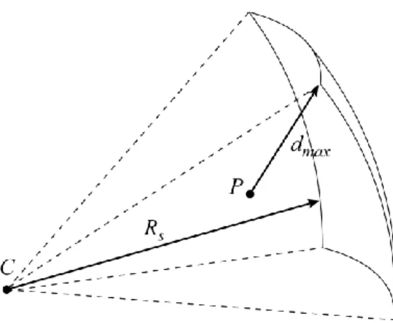
In error analysis, the intervals of interest are extremely small compared to the overall dimensions of the robot, and so is the uncertainty zone for a given nominal configuration. This means that, in practice, the radius of a portion of a sphere or a cylinder (a plane is a portion of sphere or cylinder of infinite radius) that belongs to the boundary of the uncertainty zone will be much greater than the maximum position error. Therefore, for such a tiny portion of large radius, the point that is farthest from the nominal position will be at one of the extremities of the portion. This is illustrated on Fig. 1, where Rs represents the sphere radius

For spatial robots the point that is farthest from the nominal position will be at the intersection of three portions of spheres. This point will therefore correspond to three active-joint variables at a limit.

Fig. 1. Maximal distance of a point to a portion of sphere.

Thus, thanks to this geometric analysis, we were able to demonstrate that the maximum position error cannot be elsewhere but on the thirty two edges of the input error bounding box. The only exceptions to our rule of thumb which exist will appear near singular configurations or for special designs of manipulators for which the vertex space is limited to small spheres, torus or cylinders of which radius is close to zero. But they are extremely rare and occur only for some particular mechanism designs (unknown by the authors of this paper). Moreover, the Quattro, the most used 3T1R fully-parallel robot, does not figure among the exceptions, so its maximal position errors will always be at the edges of the input error bounding box.

So, let us now observe the apparition of maxima of the fourth kind. For legs j, k and l (j, k, l = 1, 2, 3, 4, i jk l), the condition for having a maximum of the fourth kind on the interval



q_i0,q_i0 



is that:

a) X/q_i 0;

b) X/qi is orthogonal to XX0.

Condition (a) has already been discussed. Such a configuration has to be examined in order to determine whether it corresponds to a global maximum or not. However, it is very difficult to analytically identify such configurations. Therefore, once again, we are confident that the best way to proceed, in areas of the workspace where one feels that the robot might be in configurations in which three leg forces fj (j = 1, 2, 3 or 4) intersect at the centre of the

mobile platform, is to discretize the edges of the input error bounding box, compute X at

each discrete point, and retain the maximum value. Note, however, that in most cases it will be obvious that such configurations cannot occur. For these cases, one must only consider condition (b).

Condition (b) is even more complicated to analyze. The partial derivative X/qi

represents the first three elements of the ith column of the Jacobian matrix of the robot. If the direction of vectors X/q_i is close to a constant in the interval studied (which is far from Type 2 singularities), then it is possible to say that on this interval, the displacement of the robot, when legs j, k and l are fixed, is close to a straight line. This can be verified approximately by computing vector X/qi at each corner of the input-error bounding box. If

the variation of the direction of the vector X/q_i is inferior to a given value (for example 1 degree), then one can consider that the direction of X/qi does not change in the interval

studied.

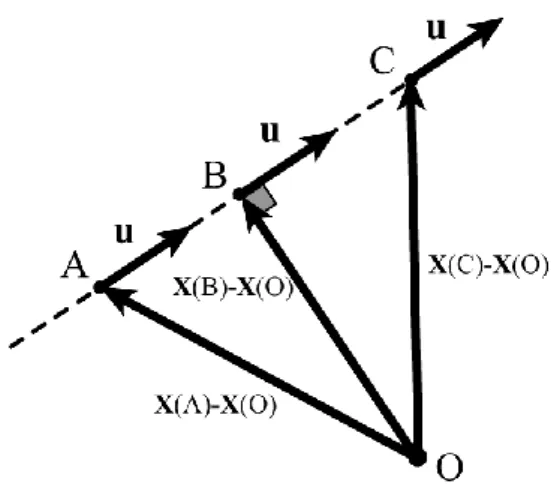
Let B be a point for which X/q_i is orthogonal to XX₀ (Fig. 2). Vector udefines the direction of the allowed displacement at point B. If we represent a line passing through

displacement of the platform around point B when only the ith actuator is moving. If we represent two points A and C located on this line around B, the direction of vector u defines the direction of the displacement when the ith leg is actuated in the positive sense of qi. Thus,

point A represents the point before passing point B and point C the point after when the ith actuator is moving.

It is so possible to determine the signs of the product



X/q_i

 

T XX₀



at points A and C. At point A it is negative and at point C it is positive. This shows that point B is a local minimum of X². Thus, such a configuration does not represent a maximum of the third kind.

Fig. 2. Analysis of a local extremum for which X/qi is orthogonal to



XX0



.

Of course, there are exceptions to our rule of thumb, but they are extremely rare and occur only for some particular mechanism designs. For example, consider the Quattro parallel robot. The curve described by the platform centre, when three of the actuators are blocked, is the intersection between a portion of a torus and a sphere, which is a relatively smooth curve. Therefore, if one takes a segment at whose endpoints the slope is nearly the same, this segment is clearly close to a line. However, if a more complex robot is considered, it is

possible to have a segment at whose endpoints the slope is nearly the same, yet the segment is far from linear (e.g., there is a cusp point, or a tiny loop). However, we consider that such situations are extremely unlikely to happen, and even if they do, they will occur for only certain configurations and not throughout the workspace. Therefore, for simplicity, we will exclude this small possibility from our study.

To sum up, the proposed method is very simple to implement and, for most practical 4-DOF 3T1R robot designs, fast and accurate. For most designs, at each nominal configuration, we have to compute the direct kinematics for sixteen sets of active-joint variables, which can either be done analytically, or using a very accurate numerical method (since we are far from singularities). Thus, for computing the local maximum orientation error and local maximum position error of a 4-DOF 3T1R parallel robot for a given nominal configuration, one should, at worst, compute the direct kinematics at only 32n points (using the algorithms presented in [23]), where n is the number of discretization points on each of the edges of the input error bounding box. As already mentioned such a discretization is unfortunately somewhat time-consuming and might lead to a certain computational inaccuracy. However, relatively simple analysis can show that for a given robot design, only the sixteen vertices of the input error bounding box should be verified. Namely, for the computation of the maximum orientation error, this is the case if no three wrenches can be parallel or coplanar and lead to a local maximum, and for the computation of the maximum position error, this is the case if no three forces fj can intersect at the platform centre and the

IV. EXAMPLE: THE QUATTRO ROBOT

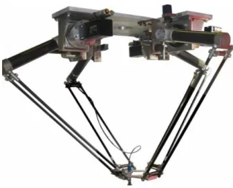
The Quattro robot is a well known Delta like manipulator [24] designed at the LIRMM of Montpellier in France (Fig. 3). The design parameters of the equivalent kinematic chain of the prototype of the LIRMM are as follows (Fig. 4):

− the actuators are mounted on the base and are located at revolute joints Ai;

− points Ai forms a square of edge length 0.5 m;

− the point O, centre of the base frame Oxyz, is taken as the centre of the square

A1A2A3A4;

− the platform is linked to the legs by four universal joints at point Ci;

− the length of the rods AiBi is 0.3 m;

− the length of the rods BiCi is 0.8 m;

− the controlled point of the platform is point P; the rotation of the tool is given by the shear of the platform which control the displacement of a pulley belt transmission linked at point P (not shown here); thus the output rotation angle is proportional to angle , therefore we consider as output angle  directly;

− the length of the rods C1C2 = C3C4 is 0.1 m;

− the length of the rods E2E3 = E1E4 is 0.1 m;

− the length of the rods DiEi is 0.01 m;

− the error bound on the active-joint variables is 4

10 2 



Fig. 3. Prototype of the Quattro (courtesy of Vincent Nabat).

(a) front view of the legs (b) Top view of the platform Fig. 4. Equivalent kinematic chain of the Quattro.

The singularities of this kind of robot are described in [21] and the authors claim that the usable workspace of their robot can be defined by at least a cylinder whose axis is vertical, centred at O and of radius equal to 0.45 m for any orientation angle. In order to avoid any computational problem due to the neighbourhood of singular positions, we restrain the radius

The direct kinematics of this robot allows up to eight real solutions and cannot be solved analytically [21]. Since we only need the solution that can be reached from the nominal pose, while the active-joint variables remain in their intervals, we will use an iterative numerical method such as the Newton-Raphson method. This method requires only the computation of the Jacobian matrix of the robot, which is very simple to obtain. In our error analysis, we will always start the algorithm at the nominal configuration and vary the active-joint variables in a very small interval of length up to ε. Furthermore, we will use this algorithm for configurations that are sufficiently far from singularities. Therefore, as verified in this example, the algorithm converges very quickly (usually, in only two iterations for a precision of 10-10 m and 10-10 degrees).

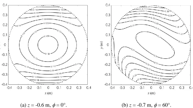
Thus, as previously said, the maximal position and orientation errors are located on the edges of the error bounding box. So it means that, for any nominal pose of the platform, there are 32n configurations to test, n being the discretization step. This is very time consuming and it would be preferable to restrain our analysis to the sixteen maxima of the fifth kind (the corner of the bounding box). In order this to be possible, we have to observe the values of the functions / q ₁ in the studied workspace (Fig. 5) as well as the variation of angle of vectors

i

q



X/ (Fig. 6). For reasons of brevity, we present only the figures for one actuator, but the values for the other actuators are very similar.

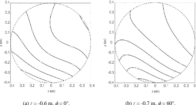
(a) z = -0.6 m,  = 0°. (b) z = -0.7 m,  = 60°. Fig. 5. Variation of function / q ₁ for two orientations and altitudes.

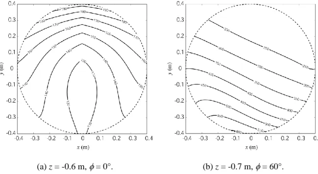
(a) z = -0.6 m,  = 0°. (b) z = -0.7 m,  = 60°.

Fig. 6. Variation in the direction of vector X/ q ₁ (degrees) for two orientations and altitudes.

It is possible to note that:

- the value of function / q ₁does not vanish in the studied workspace; - the variation in the direction of vector X/ q ₁ is very small in the studied

workspaces (less than 0.05°). As already mentioned, this is not a 100% guarantee that the maximum position error occurs at one of the eight corners of the input error bounding box. Therefore, for the purposes of this demonstration, we have also verified on the edges of the bounding box (using 20 discretization intervals on each edge). Not even one nominal configuration was found for which the maximum position error is not at one of the eight corners. Therefore, the assumption that we make is valid in this example.

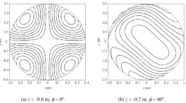
(a) z = -0.6 m,  = 0°. (b) z = -0.7 m,  = 60°. Fig. 7. Maximum orientation errors for two orientations and altitudes (degrees).

(a) z = -0.6 m,  = 0°. (b) z = -0.7 m,  = 60°. Fig. 8. Maximum position errors for two orientations and altitudes (m).

Thus, for this robot too, there only are sixteen sets of active-joint variable to test for computing the local maximum orientation error and local maximum position error of the robot. The resulting contour plots for two different orientations are presented in Figs. 7 and 8. It can be noted that the orientation error of this parallel robot is nearly constant for both orientations and altitudes. This is not the case of the position error for the orientation of the platform of 60°. This can be explained by the fact that the robot stays far from singularities in the studied workspace in the first case, and not in the second (due to the shear of the platform).

(a) z = -0.6 m,  = 0°. (b) z = -0.7 m,  = 60°.

Fig. 9. Deviation between the real and the approximate orientation error models (%) for two orientations and altitudes.

(a) z = -0.6 m,  = 0°. (b) z = -0.7 m,  = 60°.

Fig. 10. Deviation between the real and the approximate position error models (%) for two orientations and altitudes.

We also analyze the error between our exact error analysis and the values given by the first order approximation of Eq. (1) (Figs. 9 and 10). It is interesting to note that the deviation between the two models is very important in the case of the maximal position error, which is not the case for the maximal orientation error.

Finally, we measure the computation time between our analysis, for which the direct kinematics are computed sixteen times for each nominal position of platform, and an algorithm for which the error interval for each actuator are divided into ten portions. For each Fig. 7 and 8, 9600 nominal positions of the platform are tested. Our algorithm gives the solution into about 160 s (with a Pentium 4, 2.66 GHz, 2 Gb RAM). The most time-consuming algorithm will give the solution after 28 hours of computation. When testing only the edges, the results will be obtained after 50 minutes. It is clear here that our method largely decreases the computation time.

V. CONCLUSIONS

This paper presented a detailed study of the local maximum orientation and position errors occurring in 4-DOF 3T1R fully parallel robots subjected to errors in the inputs. It was proven that, when sufficiently far from singularities, the local maximum orientation and position errors can occur only when at least three inputs suffer a maximum error. However, a simple procedure was proposed to evaluate, for a given design, whether these output errors can occur when only three inputs are at a maximum error. Thanks to this detailed study, a simple method was proposed to calculate the local maximum orientation and position errors for a given nominal configuration and given error bound on the inputs. The method involves solving the direct kinematics for sixteen, or a maximum of 32n (n being the number of

simple to implement and gives valuable insight into the kinematic accuracy of parallel robot. It should be mentioned that, even if the proposed method is focused on only 4-DOF four-identical-legged 3T1R parallel robots, it can easily extended to “asymmetrical” 3T1R manipulators (typically a 6–DOF Stewart platform constrained by a passive limb with DOF less than 6). Moreover, the authors hope they will be able to extend such a work to other types of spatial parallel robots.

The authors believe that the proposed method should be used for all 4-DOF 3T1R fully-parallel robots instead of the much less meaningful dexterity maps.

REFERENCES

[1] J.-P. Merlet, Computing the worst case accuracy of a PKM over a workspace or a trajectory. The 5th Chemnitz Parallel Kinematics Seminar, Chemnitz, Germany, 2006,

pp. 83–96.

[2] J.-P. Merlet, Jacobian, manipulability, condition number, and accuracy of parallel robots. Journal of Mechanical Design 128 (1) (2006) 199–205.

[3] C.M. Gosselin, The optimum design of robotic manipulators using dexterity indices. Robotics and Autonomous Systems 9 (4) (1992) 213–226.

[4] J.K. Salisbury and J.J. Craig, Articulated hands: force and kinematic issues. The International Journal of Robotics Research 1(1) (1982) pp. 4–17.

[5] C.M. Gosselin, J. Angeles, A global performance index for the kinematic optimization of robotic manipulators. Journal of Mechanical Design 113 (3) (1991) 220–226.

[6] A. Yu, I.A. Bonev, P.J. Zsombor-Murray, Geometric method for the accuracy analysis of a class of 3-DOF planar parallel robots. Mechanism and Machine Theory 43 (3) (2007) 364-375.

[7] S. Briot, I.A. Bonev, Accuracy analysis of 3-DOF planar parallel robots. Mechanism and Machine Theory 43 (4) (2008) 445-458.

[8] S. Briot, I.A. Bonev, Are parallel robots more accurate than serial robots? Transactions of Canadian Society for Mechanical Engineering 31(4) (2007) 445–455.

[9] S. Briot, I.A. Bonev, A pair of measures of rotational error for axisymmetric robot end-effectors. Advances in Robot Kinematics, 11th International Symposium, June 22-26, 2008, Batz-sur-Mer, France.

[10] X. Kong, C.M. Gosselin, Parallel manipulators with four degrees of freedom. February 14, 2006, US Patent No. US 6 997 669 B2.

[11] Kaisha Toyoda Kokikabushiki, F. Pierrot, O. Company, Four degree of freedom parallel robot. September 18, 2000, European Patent No. EP 1 084 802 A2.

[12] L.H. Rolland, The Manta and the Kanuk novel 4-dof parallel mechanisms for industrial handling. In ASME Int. Mech. Eng. Congress, Nashville, November 14-19, 1999.

[13] Q. Li , Z. Huang, Mobility analysis of lower-mobility parallel manipulators based on screw theory. In IEEE Int. Conf. on Robotics and Automation, Taipei, September 14-19, 2003, pp. 1179-1184,

[14] S. Briot, V. Arakelian, S. Guégan, PAMINSA: a New Family of Decoupled Parallel Manipulators, Mechanism and Machine Theory, in press.

[15] G. Gogu, Structural Synthesis of Fully-Isotropic Parallel Robots with Schoenflies Motions via Theory of Linear Transformations and Evolutionary Morphology. European Journal of Mechanics / A –Solids 26 (2) (2007) 242-269.

[16] C.M. Gosselin, M. Tale Masouleh, V. Duchaine, P.-L. Richard, S. Foucault, X. Kong, Parallel mechanisms of the Multipteron family: kinematic architectures and

benchmarking. Proceedings of the 2007 IEEE International Conference on Robotics and Automation (ICRA), April 10-14, 2007, Rome, Italy.

[17] V. Nabat, F. Pierrot, M.M. De La Rodriguez, J. M. Azcoitia Arteche, R. Bueno Zabalo, O. Company, F. Perez De Armentia, Robot parallèle à quatre degrés de liberté à grande vitesse. December 12, 2007, European Patent No. EP 1 870 214 A1.

[18] J. Angeles, The degree of freedom of parallel robots: a group-theoretic approach. Proceedings of the 2005 IEEE International Conference Robotics and Automation, , April 18-22, 2005, pp. 1005 – 1012

[19] R. Clavel, M. Thurneysen, J. Giovanola, M. Schnyder, D. Jeannerat, Hita-STT, a new 5 dof parallel kinematics for production applications, ISR 2002 – International Symposium on Robotics, Stockholm, Sweden, October 07-11, 2002.

[20] C. Gosselin, J. Angeles, Singularity analysis of closed-loop kinematic chains. IEEE Transactions on Robotics and Automation 6 (3) (1990) 281–290.

[21] V. Nabat, Robots parallèles à nacelle articulée. Du concept à la solution industrielle pour le pick-and-place. Ph. D. dissertation, Montpellier, France, March 2, 2007.

[22] D. Zlatanov, I.A. Bonev, and C.M. Gosselin, Constraint singularities of parallel mechanisms. IEEE International Conference on Robotics and Automation (ICRA 2002), Washington, D.C., USA, May 11-15, 2002.

[23] J.-P. Merlet, Parallel Robots. 2nd ed., Springer, 2006.

[24] R. Clavel, Device for movement and displacing of an element in space. Patent US4976582, December 11, 1990.

Figure captions

Fig. 1. Maximal distance of a point to a portion of sphere.

Fig. 2. Analysis of a local extremum for which X/q_i is orthogonal to



XX₀



. Fig. 3. Prototype of the Quattro (courtesy of Vincent Nabat).

Fig. 4. Equivalent kinematic chain of the Quattro

Fig. 5. Variation of function / q ₁ for two orientations and altitudes.

Fig. 6. Variation in the direction of vector X/ q ₁ (degrees) for two orientations and altitudes.

Fig. 7. Maximum orientation errors for two orientations and altitudes (degrees). Fig. 8. Maximum position errors for two orientations and altitudes (m).

Fig. 9. Deviation between the real and the approximate orientation error models (%) for two orientations and altitudes.

Fig. 10. Deviation between the real and the approximate position error models (%) for two orientations and altitudes.