HAL Id: hal-01004973
https://hal.archives-ouvertes.fr/hal-01004973 Submitted on 11 Feb 2017
HAL is a multi-disciplinary open access archive for the deposit and dissemination of sci-entific research documents, whether they are pub-lished or not. The documents may come from teaching and research institutions in France or abroad, or from public or private research centers.
L’archive ouverte pluridisciplinaire HAL, est destinée au dépôt et à la diffusion de documents scientifiques de niveau recherche, publiés ou non, émanant des établissements d’enseignement et de recherche français ou étrangers, des laboratoires publics ou privés.
Accounting for variability and uncertainties in NDT
condition assessment of corroded RC-structures
Denys Breysse, Sylvie Yotte, Manuela Salta, Franck Schoefs, Joao Ricardo, Myriam Chaplain
To cite this version:
Denys Breysse, Sylvie Yotte, Manuela Salta, Franck Schoefs, Joao Ricardo, et al.. Accounting for variability and uncertainties in NDT condition assessment of corroded RC-structures. Euro-pean Journal of Environmental and Civil Engineering, Taylor & Francis, 2009, 13 (5), pp.573-592. �10.1080/19648189.2009.9693135�. �hal-01004973�
Accounting for variability and uncertainties
in NDT condition assessment of corroded
RC-structures
Denys Breysse* — Sylvie Yotte* — Manuela Salta**
Franck Schoefs*** — Joao Ricardo** — Myriam Chaplain****
* University Bordeaux 1, Ghymac
Avenue des facultés, F-33405 Talence cedex, France d.breysse@ghymac.u-bordeaux1.fr
** LNEC, Lisboa, Portugal *** University Nantes, GeM
**** University Bordeaux 1, US2B
ABSTRACT. The quantitative forecasting of corrosion development remains difficult, limiting
the development of validated preventive maintenance strategies. Difficulties come from the spatial variability of material properties, the temporal variability of the environment and the sensitivity of non destructive measurements to changing environmental conditions. The reinforced concrete Barra Bridge, Portugal, has been thoroughly investigated, and on site data have been used for modelling the development of corrosion and its variability. A model has been derived from additional laboratory experiments, which enables to account for the influence of environment and to support the decision process regarding the corrosion state and the forecasting of its evolution.
RÉSUMÉ. La prévision quantitative du développement de la corrosion demeure difficile, ce qui
limite le développement de stratégies de maintenance préventive efficaces. Parmi les sources de difficultés, on recense la variabilité spatiale des propriétés des matériaux, la variabilité temporelle des conditions environnementales et la sensibilité des contrôles non destructifs à ces conditions. Le pont en béton armé de Barra, au Portugal, a fait l’objet d’investigations approfondies. Les mesures ont été utilisées pour modéliser le développement de la corrosion et sa variabilité. Un modèle reposant sur l’exploitation de données de laboratoire complémentaires permet de tenir compte de l’influence des paramètres environnementaux et d’aider à la décision en ce qui concerne le diagnostic de la corrosion et de son évolution.
KEYWORDS: corrosion, damage, material variability, non destructive testing.
1. Introduction: difficulties with corrosion assessment in RC 1.1. Usual means for assessing corrosion
Corrosion of reinforced concrete infrastructures in marine environment, due to chloride ingress, has practical consequences on the condition and safety level of infrastructures. To reduce the cost of maintenance and repair while keeping these infrastructures at a correct level of safety, managers can use non destructive techniques to assess the condition state. When relevant models are used, life cycle cost analysis becomes possible and the maintenance of structures can be optimized (Stewart, 2005; Li, 2004). The non destructive assessment of corrosion is usually done by combining three techniques (NEA, 2002; RILEM, 2004):
– half cell potential measurements, which provide an indication of likelihood of corrosion activity at time of testing, through a value of potential (ASTM standard puts in relation the value measured and a probability of corrosion);
– measurement of the concrete resistivity, which informs about the moisture content in the concrete;
– these two first measurements give no information about the corrosion rate, which can be estimated by measuring the polarization resistance, which gives an indication of corrosion rate of the reinforcement at time of testing.
A value of the corrosion current density icorr is derived from the polarization
resistance, whose magnitude is put in relation with the corrosion state (e.g. if icorr is
lower than 0.1 μA/cm2 the steel is passive, and if it is larger than 1μA/cm2, the corrosion rate is high). The problem is however more difficult regarding interpretation. Standards only provide some information on thresholds which have to be considered as “relative thresholds” and need to be taken with a lot of care.
1.2. Uncertainties, variability and assessment
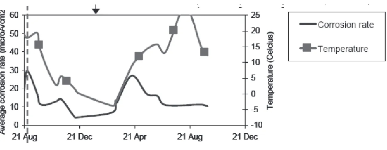
It is well known that all these techniques must be used by qualified and experienced operators, and that they mainly provide qualitative data (or relative variations) instead of quantitative ones. The main reason is that NDT only give information at the time of the measurement, and that this information is very sensitive to environmental conditions (Jäggi et al., 2001; Burgan Isgor et al., 2006), as it can be seen on Figures 1 and 2.
Continuous monitoring combined with NDT on Skovdiget bridge, near Kopenhagen has shown that, due to temperature effects, NDT inspections during automn months tend to provide conservative measurements of the corrosion potential (and thus corrosion risk). The corrosion process is itself very dependent on moisture content and temperature, which are responsible for the electrolyte continuity (pore connectivity) and for the oxygen availability at the steel surface. Moisture influences the electrical resistivity, which is the most comprehensive
parameter determining the corrosion current. Since moisture and temperature vary with time, and may also vary from place to place in the concrete, an assessment of concrete which should be independent of these variations becomes difficult. Since many influencing factors can explain any observed variability of the measurements, it is important to quantify these potential effects, such as to sort out any “real signal”, i.e. real variation with time or space, of the effective corrosion degree (Breysse et al., 2007).
Figure 1. Temporal variability of the current of corrosion (in PA) and its relation with humidity (after Klinghöfer et al., 2000)
Figure 2. Temporal variability of the average corrosion rate (in μA/cm²), showing
influence of temperature (after Samco, 2006)
Collective efforts have been undertaken in the recent years to gather data about time and space variability in relation with service life prediction and structural reliability (Duracrete, 2000). This work is based on data obtained on the reinforced concrete structure of Barra Bridge, Portugal. This bridge, located near the Atlantic Ocean, has been thoroughly investigated, for a better assessment of its corrosion state. Many non destructive and semi destructive tests have been performed on several piers, regarding reinforcement cover, half cell potential and corrosion rate measurements, concrete resistivity, chloride profiles, carbonation depth and concrete chloride diffusion coefficients. The measured on-site variability can be due either to material and exposure conditions variability or to uncertainty in the measurement process (e.g. lack of repeatability or influence of environmental conditions at the time of measurement). These two types of uncertainties have different consequences. The first one is representative of the structure and of its condition. The spatial variability of the material properties results from the construction process and concrete placing. It must be accounted for in a probabilistic approach, the residual service life becoming a probabilistic variable, whose value is distributed in the structure (Stewart, 2001; Li, 2004). The second type of uncertainties can be reduced with a more cautious approach and with the modelling of environmental effects on the measurements.
Data obtained at the laboratory, repeating for instance electrochemical measurements under varying ambient conditions, can be processed and used for this purpose. However, these measurements only provide a partial appreciation of the variability since, for on-site measurements, other factors influence the measurements: accessibility, human factors (experience, tiredness...) (Barnouin et
al., 1993). In fact, the vast majorities of probabilistic studies whose purpose is to
analyze the consequence of material variability on the structure reliability do not separate the two components of variability: the real one (aleatoric uncertainty), due to the material, and the superimposed one (epistemic uncertainty), which only comes from imperfect knowledge one has of the structure after measurement. We will try to reduce epistemic uncertainty.
It is also possible, in the well-known conditions of the laboratory, to analyze the effects of the most influencing factors on the development and monitoring of corrosion. Thus the laboratory measurements can be used to quantify the weight of the spatial and temporal variability of the main influent factors on the assessment of corrosion. This enables to partially quantify the resulting uncertainties for the on-site corrosion assessment.
2. Analysis of variability from on site investigations
2.1. Barra Bridge characteristics and investigation program
The Barra Bridge was designed by the Portuguese bridge designer Pr. Edgar Cardoso, 1971, and started operation in 1975. The bridge is located on km 0+824 of
E.N.109-7 over Ria de Aveiro. It has a 578 meters length, between the support axes on the abutments. The central span has 80 m and the access viaducts, symmetric as refers to the central span, have 249 m, each being formed by seven spans of 32 m and a last one of 25 m (Figure 3).
In a first inspection made in the Barra Bridge (in May 2006), two piers and one of the abutments were inspected. The piers were the P13 and P15, that are in land, and the abutment was the E2. The inspected zones are on the right part of the bridge (meaning right bank of the estuary, which is the farthest from the sea, since the sea is about 300 to 500 meters from the left end of the bridge. Regarding their location respectively to the river, the inspected areas on the piers are denominated as “upstream” and “downstream” (depending on what column it is referred to) and in “left” and “right” side.
So when it is said that an area is on the left side of a pier, this face is turned towards the sea and therefore more exposed to the sea winds containing chlorides. The assessment strategy was based on visual inspection which enabled to select a series of different areas (differing in elevation, part of pier and side) for further in-depth investigations. Thus measurements were performed in the selected areas, focused on concrete cover over the reinforcements, half cell potential and corrosion rate measurements.
Figure 3. Barra Bridge
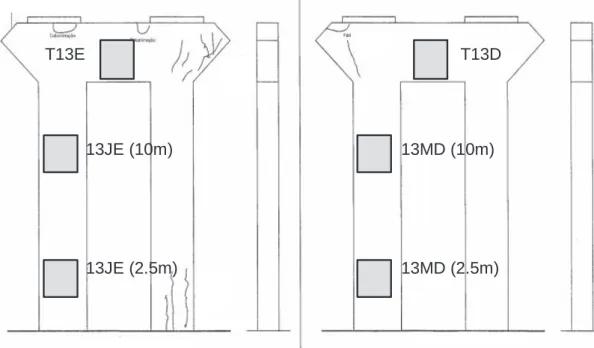
Cores were extracted for laboratory tests, mainly for chloride profiles and chloride diffusion coefficient but also for concrete compressive strength and for microstructural characterisation. In pier 13, six areas were analysed, three in the left side of the pier and three in the right side (denomination of areas is given on
Figure 4). Concrete cover, potential and corrosion rate measurements were
performed and cores were taken in five of those areas. In the last one, it has been only proceeded to concrete coring.
Figure 4. Location of investigated areas on pier 13 (left face and right face)
2.2. Spatial variability
The cover was measured using a scanning cover depth meter. The mapping of corrosion potential was performed with a Germann Instruments GD-2000 Mini Great Dane system, and the determination of the corrosion rates was done by the polarisation resistance method using the equipment GeCor 6.
The detailed results of each area, regarding the cover of each rebar, the potential values and the corrosion rate measurements were analyzed in terms of variability.
For instance, regarding the 13 MD (10 m) area (whose size is about 1 m2), the
investigation performed on 15 May 2006 has provided:
– a corrosion current density icorr in the 0.085-0.359 PA/cm 2
interval;
– a half cell potential (measured with Cu/CuSO4 reference electrode) varying
from -72.7 mV to 30.4 mV;
– a cover depth between 29 and 35 mm (horizontal rebars) and 38-40 mm (vertical rebars);
– a carbonation depth (from cores) between 10 and 14 mm.
The potential values and icorr values are not incoherent: these icorr values mean
that corrosion could be already installed; however they are not high and in case of carbonation, the concrete resistivity increases, one can have positive E values even with corrosion initiation.
Therefore, the 13 MD (10 m) area, which can be regarded as a “homogeneous” area regarding the corrosion degree (at least from visual inspection) exhibits some spatial variation of its characteristics. It is thus interesting to analyze the reasons of
13JE (2.5m) 13MD (2.5m) 13JE (10m) 13MD (10m) T13D T13E 13JE (2.5m) 13MD (2.5m) 13JE (10m) 13MD (10m) T13D T13E
this variability and to understand if it requires a statistical analysis or if it suffices to consider representative values (either mean values or conservative estimates) to have a good image of the area.
The reasons for errors in corrosion measurements have been studied by several authors. The main facts are that: each measurement depends on the more or less planeity of the concrete surface, the contact resistance between the probe and the concrete surface, the more or less symmetric positioning of the probe over the rebar, the fact that the polarization resistance has been (or not) measured after the stabilization of the potential (C-SHRP, 1995). Other limiting factors have been pointed, such as the local variability due to pitting corrosion, but the magnitude of this local variability, either due to the device or to the material, has not been thoroughly assessed. Another aspect and one of the most important is due to the effective area of steel considered for icorr calculation. When steel is passive the
confinement of electrical signal is very difficult even with the equipment used for polarization resistance measurement that facilitates the confinement. When a pitting exists, the electrical signal is totally confined to the pitting area and the estimated area is higher than actually, with consequences on the estimated icorr values.
2.3. Temporal variability and consistency
A second series of investigations was undertaken two months later (on 27 July 2006), to check the stability of the non destructive results with time, and to gather additional information. The two series of measurements have been performed in different atmospheric conditions. This information was not recorded at the time and place of the measurements and it has only been estimated afterwards:
– on 15 May 2006, the temperature was average (about 20 °C) and the weather was rather dry (RH about 80%);
– on 27 July 2006, the temperature was higher (about 25 °C) but the weather was wet (RH about 90%).
Regarding the 13MD area, the results were:
– a corrosion current density icorr in the 0.363-0.783 PA/cm2 interval;
– a potential (measured with Cu/CuSO4 reference electrode) varying from –
47.5 mV to -17.3 mV.
This shows that the non destructive results (corrosion current density or potential) cannot be simply viewed as reference values, which can be compared to normalized threshold, and that a correct assessment of the structural condition requires a lot of care. It is well known that the environmental context (mainly temperature and humidity) can influence the electrical response of the structure.
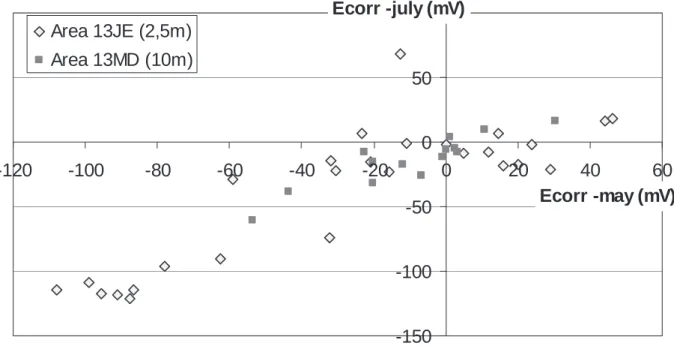
However, the repeatability of the NDT measurements can be checked by comparing the two series of measurements (Figure 5). On these two areas, 13JE (2.5 m) and 13MD (10 m), the overall consistency between the two series of
measurements is good, even if each one has some scatter. The “local noise” which corresponds to the scatter is about +/- 15 mV. Similar conclusions can be drawn for others areas. -150 -100 -50 0 50 100 -120 -100 -80 -60 -40 -20 0 20 40 60 Area 13JE (2,5m) Area 13MD (10m) Ecorr -july (mV) Ecorr -may (mV)
Figure 5. Repeatability of potential measurements at the same points (in mV) for
two areas
Regarding the measured values for the corrosion current density, they are very different for the two series of measurements, as summarized in Table 1.
Table 1. Average values for icorr (μA/cm²) measurements at two different times
Area May July Difference (%)
13 JE 0.31 0.62 + 98
13 MD 0.31 0.53 + 75
13 – : T beam 0.22 0.48 + 123
all 0.29 0.54 + 86
The average value of icorr has been multiplied by about 2 between May and July
(multiplying factor = 1.86 calculated on 11 measurements on Pier 13).
2.4. Cover depth variability
All data regarding cover have been synthetized, such as to quantify the variability at various scales (within an area, within a pier, for the whole bridge). A significant difference has been noted between horizontal and vertical rebars (due to obvious design reasons), with an average cover depth which is 7 to 8 mm larger for
vertical rebars. A significant difference has also been noted between Pier 13 and Pier 15, which can only be explained by the variability in the rebar positioning:
– Pier 13: average horizontal cover depth 29.1 mm, average vertical cover depth 37.7 mm;
– Pier 15: average horizontal cover depth 37.3 mm, average vertical cover depth 44.8 mm.
No difference was noted regarding the “upstream” or “downstream” position, or the “left” or “right” position. Thus the quantified variability only regards that of a set which would normally be a constant value.
More detailed measurements of cover depth have been performed during the second series of investigations, to quantify the longitudinal variation of cover depth along a given rebar. For instance, one has measured between 30 and 35 mm when the cover depth had at first been estimated as being 34 mm. The coefficient of variation (c.o.v.) along a rebar is between 3 and 10% for a length of about one meter, with an average value of 7%. This value can also be compared with what is considered as the accuracy of the measurement, which is assumed about plus/minus 2 mm or 5% when measuring covers to bars of known diameter under all realistic site conditions (Alldred, 1996). However, round robin test have shown larger deviations, with errors reaching 10 mm and more (Hamasaki et al., 2003). With such values, it would be difficult to tell if the measured variation along a rebar is only due to imperfect measurements or if it has a real cause in the rebar positioning. However, in our case, the real location of reinforcements was further observed during the repair phase, and the expected variations were confirmed by observation.
For a given 1 m2 area, and a given set of rebars (horizontal or vertical) the c.o.v. ranges between 9 and 16%. This c.o.v. sums the variance along the rebar and the variance between the rebars. It amounts to 20 to 30% if one combines the two directions of reinforcements in a given area. This value is much larger than that of an individual rebar. When a whole pier is considered, the coefficient of variation is about 30%.
3. Laboratory experimental program 3.1. Analysis of influent factors
Moisture content in the concrete and environmental humidity are the most influencing factors affecting the corrosion development, but also the electrochemical parameters assessed via non destructive techniques (Lataste et al., 2005). It is also well known (Andrade and Alonso, 1996; Gonzalez et al., 1996) that other influencing factors are the quality of concrete, the chloride content, the oxygen content. Since the measurements are also performed through the cover concrete, the cover depth also appears as an influent parameter. Thus an experimental programme
has been designed such as to quantify the influence of some of these parameters on the corrosion development and on the current of corrosion.
Specimens were cast with two w/c ratios (0.45 and 0.65) and two cover depths
(1 cm and 3 cm). Two prisms with 20x20x25 cm3 were prepared for each concrete
type and cover depth. Chlorides have also been added to the mix, such as to ensure the initiation of corrosion (3% total chlorides related to cement content).
0,00E+00 1,00E+03 2,00E+03 3,00E+03 4,00E+03 5,00E+03 6,00E+03 7,00E+03 0 40 80 120 160 200 240 280 320 Tempo (dias) vco rr ( m/ a n o ) 0 10 20 30 40 50 60 70 80 90 100 BCl1A BCl1B T HR T(°C) and HR (%)
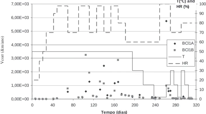
Figure 6. Measurements of icorr on two specimens (A and B) of the same mix
All specimens were subjected during ten months to varying conditions regarding relative air humidity (20% < RH < 100%) and temperature (2 °C < T < 50 °C). Regular measurements of polarization resistance have been performed, from which corrosion current density has been deduced. An example of measurements results is given on Figure 6 for two specimens denoted A and B (w/c = 0.65, cover = 1 cm).
3.2. Modelling of corrosion current density
Statistical analysis has been performed on the whole series of measurements, such as to identify the most influencing factors and to provide, via multilinear regression analysis, a quantitative model for icorr (given in PA/cm²). The variations
of icorr are the result of the combined influence of many parameters due to
environmental conditions (T and RH), to concrete (w/c and d) and time. There is also probably some “noise” due to the non perfect reproducibility of the measurement, but it is included in the overall variability. The purpose is therefore to identify an empirical model explaining as most as possible the experimental variance of icorr. Due to the fact that the icorr values can vary in a large range, ln(icorr)
V
corr (&
m/a
no
values have been considered in the model. Our choice has been that of fitting a multilinear regression model on the whole data set.
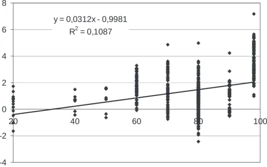
As it was expected from previous studies, moisture is the most important parameter. Figure 7 shows how it is positively correlated with ln(icorr.), the diagram
excluding RH = 100% values, since this value involves different physical phenomena limiting the corrosion rate: when the concrete is saturated, the corrosion rate is limited by the avalability of oxygen. The low (however significant) value of r² shows that it is important to consider the other influent parameters.
y = 0,0312x - 0,9981 R2 = 0,1087 -4 -2 0 2 4 6 8 20 40 60 80 100
Figure 7. Correlation between RH (in %, x-axis) and ln(icorr.) (y-axis)
Accounting for the linear influence of RH for explaining ln(icorr) variability
reduces by a factor of 2 the total experimental variance. The other parameters bring less information but the effect of temperature, cover depth and water to cement ratio are significant. Each of them leads to an additional reduction of variance of about 10%. It has been checked that the two other parameters (total time since the beginning of experiment, and time elapsed since the beginning of the new level of (RH, T) are not statistically significant). This probably comes from the experimental process, in which only short duration steps have been applied, the (HR, T) values being frequently modified (see Figure 6).
The multilinear regression analysis leads to:
ln icorr = 0.0312 RH – 4736/T + 1.695 w/c – 0.391 d + 14.589 [1]
icorr = A e
0,0312 RH
e -4736/T e -0.391 d e + 1.695 w/c [2] where:
– RH is the air relative humidity (in %); – T is the air temperature (in K);
– d is the cover depth (in cm); – w/c is the water to cement ratio; – A is a constant (in PA/cm2).
This empirical model quantifies the combined influence of the four parameters (RH, T, d, w/c) on the measured value of the corrosion current density. The unexplained variance of the model which accounts for the combined influence of these four parameters is only 36% of the total experimental variance, giving an idea of the “quality” of this model. It must be added that the model can only be used for RH < 100%, since when the concrete is saturated the involved mechanisms are different. It thus makes possible the correction of the measurements to cancel the effects of these parameters when they are varying with time and/or space.
Another expression can be identified if one considers renormalized (i.e. within the [-1, +1] range ) variables X’ with:
X’ = (2 X – Xm – XM) / (XM- Xm) [3]
where Xm and XM are respectively the minimum and maximum values of X given at
Section 3.1. It thus comes:
ln icorr = 0.2524 RH’ – 0.2654/T’ + 0.0352 (w/c)’ – 0.0812 d’ – 0.342 [4]
When it is compared with Equation [2], Equation [4] presents the advantage of being without dimension. Thus the coefficients in front of each parameter give the relative influence of each factor. This confirms that the corrosion current density is larger when RH increases, T increases and d decreases. It also confirms that the temperature and moisture are the most influencing parameters. For instance:
– it is multiplied by a factor 1.37 if RH varies from 80% to 90%; – it is multiplied by a factor 1.70 if T varies from 15 °C to 25 °C; – it is multiplied by a factor 1.48 if d varies from 3 cm to 2 cm.
4. Assessing uncertainties
4.1. Principle of a correction factor
Let us set aside the influence of the concrete mix (described in the model through the w/c parameter), and let us focus on the influence on the icorr measured
value (for a given concrete) of the variation of the dominant factors quantified above : RH and T as environmental parameters and the cover depth.
One can define an arbitrary reference set Sref = {RHref, Tref, dref} and consider the
real set S = {RH, T, d} at the place and time of the measurement. Since icorr is
measured with S, the question is to correct it (using a multiplying factor), such as to
obtain an icorr ref reference value which would have been measured under the
conditions of the reference set. The obtained reference value would then be independent of any time variation in the environmental conditions (temperature, humidity) as well as of any spatial variation in the cover depth of rebars. Writing Equation [2] a first time for the real set S and a second time for the reference set Sref,
thus eliminating A, it comes:
icorr ref = k icorr [5]
with:
k = e0,0312 (RH – RHref) e-4736( 1/T – 1/Tref) e -0,391 (d - dref) [6] One has to note that the choice of the reference set is arbitrary and has no consequence on the method itself. It is only a simple mean to compare two measurements which have been performed in different conditions, which would normally prevent any direct comparison.
4.2. Effects of temporal and spatial variability Table 2. Correcting factor on icorr for several sets
RH (%) T (°C) d (cm) k 65 20 3 1.597 95 20 3 0.626 80 5 3 2.390 80 35 3 0.455 80 20 2 0.676 90 25 3 0.558
(reference set = {RHref = 80%, Tref, = 20°C, dref = 3cm})
Considering the following arbitrary reference set: Sref = {RHref = 80%, Tref, =
293K, dref = 3 cm}, one can calculate the correcting factor for any set at the time and
place of measurement. The Table 2 gives some examples of such correcting factors for various sets. The last line on Table 2 gives the factor (k = 0.558) by which one would have to multiply the July measurements (see Section 2.3) to compare them with the May measurements which had been realized in the Sref reference conditions.
lack of any more accurate record of atmospheric conditions prevents us to conclude further on this point.
Equation [6] giving k value can also be helpful in interpretating the level of significance of any spatial variation which can be noted on site, when T and RH can be assumed as constant (during the series of measurements). Variations in measured values of icorr can be due either:
– to a different degree of intensity of corrosion, which is the purpose of NDT measurement;
– to the variation of an influent parameter, like the cover depth;
– to the variation of any other influent parameters (for instance local microstructure of concrete) or to any noise in the measurement process.
It is easy to quantify the variability on icorr resulting from any variability on the
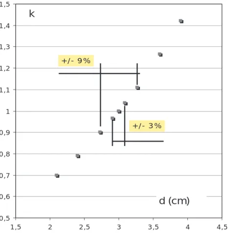
cover depth. The cover depth variability has been assessed on the Barra Bridge at three scales: that of a given rebar, that of a 1 m2 area (Area 13MD for instance), that of the whole series of measurements on a given Pier (Pier 13 for instance), all rebars being combined in the same population. Table 3 summarizes the measurement results. 0,5 0,6 0,7 0,8 0,9 1 1,1 1,2 1,3 1,4 1,5 1,5 2 2,5 3 3,5 4 4,5 d (cm) k +/- 3% +/- 9%
Figure 8. Correction coefficient k for the variation in icorr around a reference value
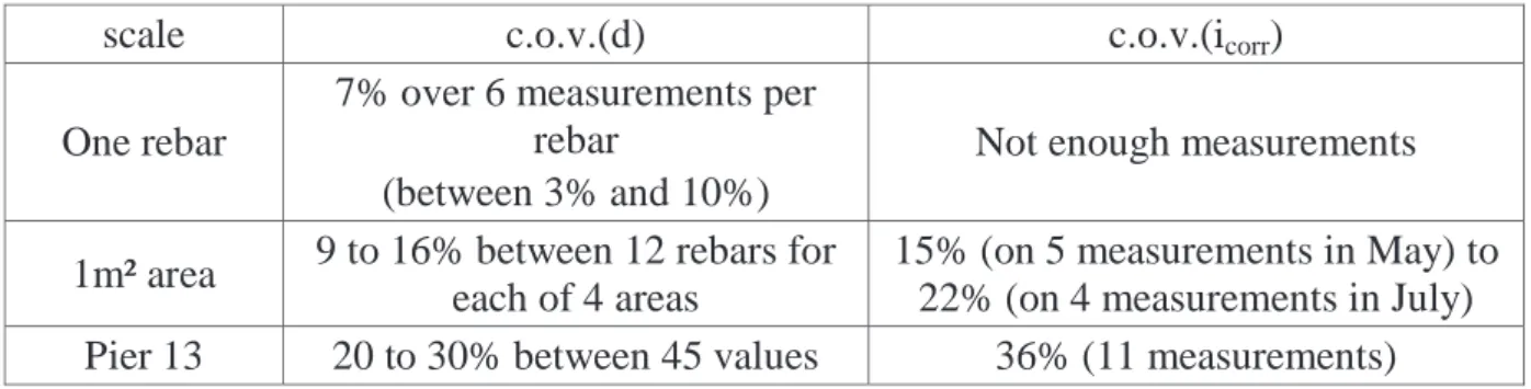
Table 3. Measured variabilities of cover and of corrosion current density at three
scales (c.o.v. indicates coefficient of variation)
scale c.o.v.(d) c.o.v.(icorr)
One rebar
7% over 6 measurements per rebar
(between 3% and 10%)
Not enough measurements
1m² area 9 to 16% between 12 rebars for each of 4 areas
15% (on 5 measurements in May) to 22% (on 4 measurements in July)
Pier 13 20 to 30% between 45 values 36% (11 measurements)
Figure 8 shows what variation in the corrosion current density can be expected as a result of the measured variability on cover depth (independently from any variability in the environmental conditions and noise measurement), and taking d = 3 cm as a central reference value as selected before. It appears that the measured variability (c.o.v. = 36% at the scale of the pier) can logically be expected as a consequence of the simple variability of cover depth at the same scale.
4.3. Interpretation of measurements and structural assessment
Bordeaux 2006 0 1 2 3 4 5 6 7 8 24/11/ 2005 24/12/ 2005 23/01/ 2006 22/02/ 2006 24/03/ 2006 23/04/ 2006 23/05/ 2006 22/06/ 2006 22/07/ 2006 21/08/ 2006 20/09/ 2006 20/10/ 2006 19/11/ 2006 19/12/ 2006 18/01 2007 K
Figure 9. Daily variation of correcting factor k
All variations observed during the corrosion current density measurements (between two series in May and July, and within each series) can be explained as being a consequence of the spatial and/or temporal variations of measurable influent parameters. Waiting for alternative explanations, it seems therefore reasonable to
consider that the corrosion degree has not significantly increased between the two series and is homogeneous at the spatial scales investigated.
We can also apply the empirical model of Equation [6] to the question of the representativity of a punctual measurement of corrosion rate. For this purpose, we have used meteorological chronicles recorded in the city of Bordeaux, France, which is located 40km from the Atlantic Ocean, in atlantic climate. For the year 2006, we have considered average daily temperature and air moisture and computed the value of k coefficient according to Equation [6]. The result is provided on Figures 9 and 10. One has to keep in mind that k is the correcting multiplying factor that must be applied to the measured value such as to obtain “what would have been obtained under” reference condition measurements.
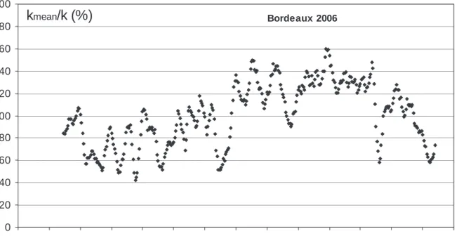
Bordeaux 2006 0 20 40 60 80 100 120 140 160 180 200 24/11 /2005 24/12 /2005 23/01 /2006 22/02 /2006 24/03 /2006 23/04 /2006 23/05 /2006 22/06 /2006 22/07 /2006 21/08 /2006 20/09 /2006 20/10 /2006 19/11 /2006 19/12 /2006 18/01 /2007 kmean/k (%)
Figure 10. Ratio between kmean (yearly average of k) and k (averaged on 1 week)
Figure 9 shows that the k value varies in a large range, from less than 1 during summer (the meteorological conditions approaching the reference ones) to more than 4 or 5 on some dry and cold days of winter and spring. The average value over the whole 2006 year equals kmean = 1.72. If one considers that, for active corrosion,
icorr is directly proportional to the steel loss, this value is representative of the
corrosion intensity over the year. Thus any isolated measurement of icorr, during a
“random” day, only provides a random estimation of this corrosion intensity, which is an overestimation if the measurement is performed during summer (corrosion is, in our case, more active than average between mid-june and end of October) while it is an understimation if it is provided at other periods. Figure 10 highlights this point by quantifying the kmean/k ratio, which can be put in parallel with the relative
corrosion activity along time. Figures 9 and 10 are in total agreement with what was illustrated on Figures 1 and 2 from on-site monitoring of structures.
Thus the model opens an easy way for a more reliable assessment of corrosion, enabling to replace the results of measurements obtained at any time in a wider panorama, being assumed that meteorological information (at the time of the measurements as well as for the usual service condition) are known.
4.4. Generalizing the approach
The correction factor expression Equation [6] has been fitted from the laboratory experiments and it remains an empirical factor. One has all reasons to think that it would have been slightly different with another concrete mix. However, the expression can be assumed to be, more generally:
k = e a (RH – RHref) e - b( 1/T – 1/Tref) e - c (d - dref) [7]
a, b and c being positive constants which would have to be fitted in any particular case (given structure, given concrete, given history...). The strategy to fit their value is however simple. It would be enough, on the studied structure, to monitor the current of corrosion under varying ambient conditions (24 hours would suffice to have varying T, and perhaps few weeks to cover a wide range of variations for RH). Thus a and b can be derived from the regression between icorr, RH and 1/T.
5. Conclusions
The combination of on site investigation and the analysis of an experimental laboratory program has shown how to assess the time variability of corrosion rate and how to improve the diagnosis.
A model has been derived from the laboratory experiments. It shows how the corrosion current density is highly sensitive to the environmental conditions, mainly the relative air humidity. It enables the derivation of a correcting factor which can be used to predict the values of the corrosion current density which would have been measured, notwithstanding any uncontrolled variation of the environmental conditions (HR and T).
The same model also describes the influence of the variability of the cover depth, which can easily be assessed on site. Since usual variations in the cover depth range in the (-30%, +30%) around nominal values, it is relevant to calculate the consequences of these variations. Thus, the combination of the two measurements (current of corrosion and cover depth) at the same point enables an easy correction, and provides more relevant information on the degree of corrosion. In both cases, the assessment of the degree of corrosion will be improved. This can improve the steel loss assessment, providing more accurate information for the residual service life assessment of the structure.
The model developed in this paper cannot be seen to be universal and further studies must be undertaken so as to build robust models, which can be used for correcting efficiently the series of rough measurements obtained on corroded structures. It will also help the users in understanding the reasons for variations between several series of measurements and, prevent them from deducing that observed variations are always a consequence of a real varying activity of corrosion. Acknowledgements
This work has been developed in the frame of the European Interreg IIIb-Atlantic space program, Medachs project (Project 197).
6. References
Alldred J.C., 1996, Rebar location and cover measurement to aid corrosion potential surveys, Inter/Corr96, http://www.corrosionsource.com/
Andrade C., Alonso C., “Corrosion rate monitoring in the laboratory and on-site”,
Construction and Building Materials, vol. 10, n° 5, July 1996, p. 315-328.
ASTM C876-91, Standard test method for half-cell potentials of uncoated reinforcing steel in concrete, 1999.
Barnouin B., Lemoine L., Dovetr W.D., Rudlin J., Fabbri S., Rebourcet G., Topp D., Kare R., Sangouard D., “Underwater inspection reliability trials for offshore structures”, Proc. 12th
Int. Conf. On Offshore Mechanics and Arctic Eng., ASME, vol. 2, 1993, p. 883-890.
Breysse D., Yotte S., Salta M., Pereira E., Ricardo J., Povoa A., Influence of Spatial and
Temporal Variability of the Material Properties on the Assessment of a RC Corroded Bridge in Marine Environment, ICASP 10, Tokyo, ed. Kanda, Takada, Furuta, Taylor &
Francis, 31 July-3 August 2007, p. 543-544.
Burgan Isgor O., Ghani Razaqpur A., “Modelling steel corrosion in concrete structures”, Mat.
Str., vol. 39, 2006, p. 291-302.
C-SHRP, 1995, Measuring the corrosion rate of reinforcing steel, Canadian Strategic Highway Research Progress, Techn. Brief #6, June 1995.
Duracrete, “Statistic quantification of the variables in the limit state function”, Brite EURAM
Project, vol. 111, 2000.
Gonzalez J.A., Feliu S., Rodriguez P., Ramirez E., Alonso C., Andrade C., “Some questions on the corrosion of steel in concrete – Part I: When, how and how much steel corrodes”,
Mat. Str., vol. 26, 1996, p. 40-46.
Hamasaki H., Uomoto T., Ohtsu M., Ikenaga H., Tanano H., Kishi K., Yoshimura A., Identification of reinforced in concrete by electro-magnetic methods, NDT-CE 2003, Berlin, 2003.
Jäggi S., Böhni H., Elsener B., “Macrocell corrosion of steel in concrete – experiments and numerical modelling”, Eurocorr. 2001, Riva di Garda, Italy, 1-4 October 2001.
Klinghöfer O., Frolund T., Poulsen E., “Rebar corrosion rate measurements fir service life estimates”, ACI Fall Convention 2000, Committee 365, Practical Application of Service
Life Models, Toronto, Canada, 2000.
Lataste J.F., Balayssac J.P., François D., Olivier G., « Méthodes électriques et
électrochimiques », chap. B6, Méthodologie d’évaluation non destructive des ouvrages en
béton armé, Breysse D., Abraham O. (ed.), Presses ENPC, 2005, p. 275-304.
Li Y., Effect of spatial variability on maintenance and repair decisions for concrete structures, Master Sc., Tsinghua Univ., Hunan, China, 2004.
NEA, 2002, Electrochemical techniques to detect corrosion in concrete structures in nuclear installations, Nuclear Energy Agency, OCDE Technical note 21, 19 July 2002.
RILEM, Recommendations of RILEM TC-154-EMC: “Electrochemical techniques for measuring metallic corrosion”, Test methods for on-site corrosion rate measurement of steel reinforcement in concrete by means of the polarization resistance method, C. Andrade, C. Alonso, J. Gulikers, R. B. Polder, R. Cigna, Ø. Vennesland, M. Salta, Mat.
Str., vol. 37, n° 273, 2004, p. 623-643.
Samco, Work Package 9: Practical bridge management – Interface with current practice, SAMCO Project, final report on Bridge Management, March 2006.
Stewart M.G., “Risk based approaches to the assessment of ageing bridges”, Reliability
Engineering and System Safety, vol. 74, n° 3, 2001, p. 263-273.
Stewart M.G., Life-cycle cost analysis considering spatial and temporal variability of corrosion-induced damage and repair to concrete surface, ICOSSAR 2005, Millpress, Rotterdam, 2005, p. 1663-1670.