Caractérisation de la nature physique du rejet d’un évent en cas d’emballement de réaction : étude du modèle de désengagement

(1)

HAL Id: tel-01844260

https://tel.archives-ouvertes.fr/tel-01844260

Submitted on 19 Jul 2018

HAL is a multi-disciplinary open access archive for the deposit and dissemination of sci-entific research documents, whether they are pub-lished or not. The documents may come from teaching and research institutions in France or abroad, or from public or private research centers.

L’archive ouverte pluridisciplinaire HAL, est destinée au dépôt et à la diffusion de documents scientifiques de niveau recherche, publiés ou non, émanant des établissements d’enseignement et de recherche français ou étrangers, des laboratoires publics ou privés.

Caractérisation de la nature physique du rejet d’un

évent en cas d’emballement de réaction : étude du

modèle de désengagement

Jie Xu

To cite this version:

Jie Xu. Caractérisation de la nature physique du rejet d’un évent en cas d’emballement de réaction : étude du modèle de désengagement. Autre. Université de Lyon, 2017. Français. �NNT : 2017LY-SEM024�. �tel-01844260�

(2)

N°d’ordre NNT : 2017LYSEM024

THESE de DOCTORAT DE L’UNIVERSITE DE LYON

opérée au sein de

l’Ecole des Mines de Saint-Etienne

Ecole Doctorale

N° 488

Sciences, Ingénierie, Santé

Spécialité de doctorat

: GENIE DES PROCEDES

Soutenue publiquement le 09/10/2017, par :

Jie XU

Caractérisation de la nature physique

du rejet d’un évent dans le cas d’un

emballement de réaction : étude du

modèle de désengagement

Devant le jury composé de :

HERRI Jean-Michel, Professeur, Mines Saint-Etienne Président AUGIER Frédéric, Ingénieur de Recherche, IFPEN Rapporteur

LAURENT André, Professeur Émérite, ENSIC Rapporteur

CAMEIRAO Ana, Maitre Assistant, Mines Saint-Etienne Directrice de thèse

GUINAUDEAU Aymeric, Ingénieur, SOLVAY Invité

(3)

(4)

To

my beloved parents

and

(5)

Be not afraid of life,

Believe that life is worth living,

And your belief will help create the fact.

From William James

(6)

Acknowledgement

After all the academic parts, finally, it is time to complete my dissertation by this last section, to address express my sincerely thanks of gratitude to everyone for all your support and encouragement. Without you, this work would not have been possible.

Thanks to my committee members who were more than generous with their experience and precious time. A special thanks to my referees: M. Andre Laurent and M. Frederic Augier for their hours of reading, examining and reflecting of this work.

Thanks to my supervisors Ms. M. Jean-Pierre Bigot, M. Jean-Michel Herri and especially Ms. Ana Cameirao, for the prompt inspirations, excellent scientific suggestions, dynamism and kindness, which have enabled me to accomplish my thesis.

Thanks to my industrial tutors M. Sebastion Righini, Ms. Wassila Benaissa, and M. Aymeric Guinaudeau, in name of Solvay, for giving an industrial perspective about the results, and for their timely advice and co-operation throughout my study.

Thanks to the collaboration of INERIS: Ms. Claire Villemur and Ms. Patrica Vicot for realizing several interesting tests for this thesis.

Thanks to the technical teams of EMSE, for providing all the necessary technical support for this thesis with their excellent competence: Fabien, Alain, Richard, Marc, Marie-Claude, Jean-Pierre, Jérome, Frédéric, Andrée-Aimée.

Thanks to the team SP2 and AROMA of Solvay: Morad, Noel, Florian, Clement, Daniel for their kind help and valuable suggestions.

Thanks to the coffee time!

A special thanks goes to my colleagues, my friends for your presence, your support, your jokes, and your energy which makes me a joyful and rich PhD life. So, you are: Xavier – super video man, very helpful for combining the video with the curves, which makes my presentations more interesting; Maxym – the only “roux” I shared the office with; Mariana – super dancer and great traveler; Agathe – welcoming me on my first PhD day with a warm smile; Jerôme – offering wonderful computer service and chocolate; Carole – refunds, purchases and love; Hervé – the “blond”; Fayssal – he

(7)

knows everything! My administrative supporter for my residence permit; Joao – you like red wine, and me too; Mathilde – cakes, chocolate and sport; Sylvain or Martin the “stagiaire” – guarantor and singer of Mulin; Carolos – outstanding scientist; Hao – a friend I can speak Chinese with; Solmaz – we went to sports room together.

Thanks to my other friends for the friendship and for the moments we spent together.

Thank to my Mickeal, for his understanding, his sense of humor and constant encouragement.

The last, I would like to thank my parents, whose love and guidance are with me in whatever I purse.

(8)

List of Symbols

English letters

A ideal cross-section area of emergency vent m2

A pro-exponential factor in Arrhenius equation l.mol-1_.s-1

Ar cross-section area of reactor m2

C concentration mol.l-1

C0 distribution parameter (-)

CD flow rate coefficient (-)

Cp heat capacity of liquid at constant pressure J.kg-1_.K-1

D vessel or pipe diameter m

Db bubble diameter m

DI diameter of stirrer impeller m

DH hydraulic diameter m

DH* dimensionless hydraulic diameter (-)

Ea activation energy kJ.mol-1

Factor additional heat transfer coefficient W K-1

Flg gas flow rate number (-)

Fr Froude number (-)

g gravitational acceleration m s-2

G mass velocity of flux, mass flow rate per unit area kg.s-1_.m-2

h specific enthalpy of fluid in the vessel J.kg-1

hfg enthalpy of vaporization J.kg-1

H total height of swelled liquid m

(13)

Hr height of the vessel m

j total volumetric flux of the mixture m.s-1

jg gas superficial velocity (volumetric flux) m.s-1

jg max gas superficial velocity at the liquid surface m.s-1

m instantaneous mass in the vessel kg

m0 initial mass in the vessel kg

ṁ specific mass production rate of gas kg gas.s-1.kg mix-1

M molar mass kmol kg-1

N stirrer rate s-1 Nμf viscosity number, = 𝜇_𝑓 _(𝜌_𝑓_𝜎_𝑓_√ 𝜎𝑓 𝑔(𝜌𝑓−𝜌𝑔)) 0.5 ⁄ (-) P system pressure Pa Po power number (-)

Power power input by stirring kW

q heat release rate per unit mass J.s-1_.kg-1

qr reaction heat release J.s-1

Q volumetric flow rate m3_.s-1

r reaction rate mol.l-1_.s-1

R gas constant J.K-1_.mol-1

Re Stirrer Reynold’s number (-)

t time s

T system temperature K or °C

U heat transfer coefficient W m-2_K-1

u component velocities m.s-1

ugj drift velocity of gas relative to the volumetric flux (ug-j) m.s-1

u∞ characteristic bubble rise velocity m.s-1

V volume m3

x reaction conversion (-)

(14)

z height in the vessel m

Z compressibility factor (-)

ΔHr reaction enthalpy kJ.mol-1

Greek letters

α local void fraction (-)

ᾱ average void fraction over swelled height ᾱ =_𝐻1∫ ≪ 𝛼 ≫₀𝐻 𝑑𝑧

(-)

αi void fraction in vent line (-)

αmax void fraction in the liquid-vapor mixture surface (open

system) (-)

ᾱ max maximum average void fraction during a runaway venting (-)

𝛾 ratio of specific heat capacity Cp/Cv (-)

ρ density kg.m-3

σ surface tension N.m-1

ʋ Special volume of vapor kg.m-3

µ viscosity mPa.s

𝜙 Phi factor (-)

Ψ dimensionless gas superficial velocity at the liquid surface ψ jg∞ /u∞

(-)

Subscripts & Operators

0 initial

ad adiabatic

amb ambient

bottom reactor cross section

c center line for correlations or critical for mixing rule

f liquid phase

j, je,js jacket, inlet & out of jacket

(15)

i vent line

ii component ii for mixing rule

max liquid-vapor mixture surface in correlation and maximum in energy balance

meas measurement pc pseudocritical r reactor TH theoretical w pipe wall wet wetting <> _{average value < 𝑓 >=} 1 𝐴𝑅∫ 𝑓𝑑𝐴𝐴𝑅

<<>> _{weighted mean value ≪ 𝑓 ≫=}<𝛼𝑓> <𝛼>

(16)

Glossary

AA (PAA) Acrylic acid (poly acrylic acid)

AcAc Acetic acid

AcAn Acetic Anhydride

Blowdown Rapid discharge of a vessel

Bubbly flow Disengagement flow pattern in a vessel: almost uniform bubble size

Churn-turbulent flow Disengagement flow pattern in a vessel with a large distribution of bubble size

DIERS Design Institute for Emergency Relief Systems

DMSO Dimethyl sulfoxide

ERS Emergency Relief System

Ester Methyl Acetate

GC Gas chromatography

Kiwi reactor 0.5 l Visualization reactor in Solvay

MeOH Methanol

NMR Nuclear Magnetic Resonance Spectroscopy

PEO Polyethylene oxide

PVP Polyvinylpyrrolidone

SDS Sodium dodecyl sulfate

Similarity vent screening tool Vent Sizing by venting experiments which measures the mass change during the evacuation.

UN reaction 10 l pilot for direct vent sizing analysis

VSP2 pseudo-adiabatic calorimeter: Vent Sizing Packaging II

% n/n mole ratio

(17)

(18)

List of Figures

Figure I-1 Pressure relief valve ... 12

Figure I-2 Bursting disc before and after a rupture ... 13

Figure I-3 Venting flow nature ... 14

Figure I-4 Different thermodynamic systems ... 15

Figure I-5 Dramatic effect of allowing for overpressure (Fauske, 2006) ... 19

Figure I-6 One traditional flow regimes in small pipes (Ashfaq Shaikh and Muthanna H. Al-Dahhan, 2007) ... 22

Figure I-7 Two main types of bubbly flow in large pipes (Kataoka, Isao and Serizawa, Akimi,Thermopedia) ... 23

Figure I-8 Flow pattern depends on the void fraction signal (Schlegel et al., 2009) ... 23

Figure I-9 Scheme for determining flow regime(Etchells and Wilday, 1998) ... 25

Figure I-10 Bubble packing and coalescence pattern (Friedel and Wehmeier, 1991) ... 26

Figure I-11 Void fraction in bubbly flow (Zuber & Hench (Zuber N. and Hench .J, 1962), cited in (Levy, 1999)) ... 26

Figure I-12 (a) Needle injection mixer (uniformly bubble distribution); (b) Mixer with elbow horizontal section (Hibiki and Ishii, 2001) ... 27

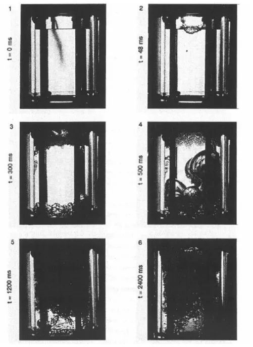
Figure I-13 Depressurization of methanol ... 29

Figure I-14 Top venting for a non-foaming and non-reactive vapor/liquid system(Wehmeier, 1994) ... 30

Figure I-15 Esterification venting ... 31

Figure I-16 Methanol/acetic anhydride esterification venting ... 32

Figure I-17 (a) Water blowdown experiment and (b) foamy water blowdown experiment 33 Figure I-18 Infinite pipe, “open” or “batch” and “closed” system ... 34

Figure I-19 Drift flow ... 35

Figure I-20 Drift velocities ... 35

Figure I-21 Flux profile ... 36

Figure I-22 Open pipe ... 38

Figure I-23 Radial distribution parameter for round bubble column (Cumber, 2002) ... 45

Figure I-24 Influence of the viscosity (Kataoka and Ishii, 1987) ... 47

(19)

Figure I-26 Variation of initial mass flow rate versus viscosity ratio... 48

Figure I-27 Thermocouple test ... 49

Figure II-1 (a) Liquid density; (b) surface tension versus temperature ... 60

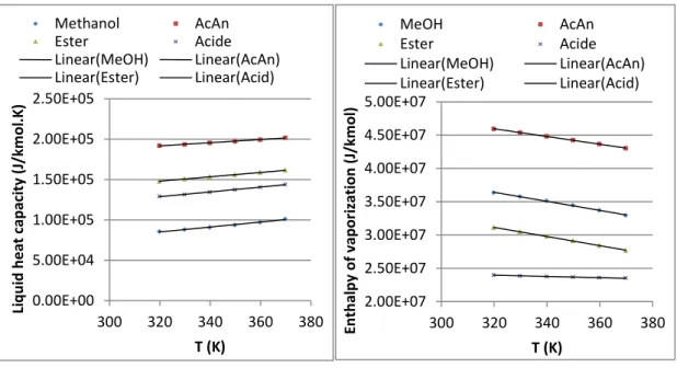
Figure II-2 (a) Liquid heat capacity; (b) enthalpy of vaporization versus temperature ... 61

Figure II-3 Structure of PVP ... 62

Figure II-4 Structure of PEO ... 63

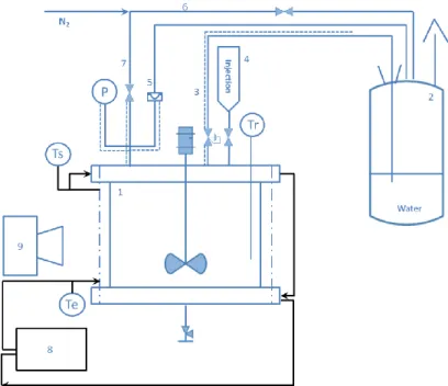
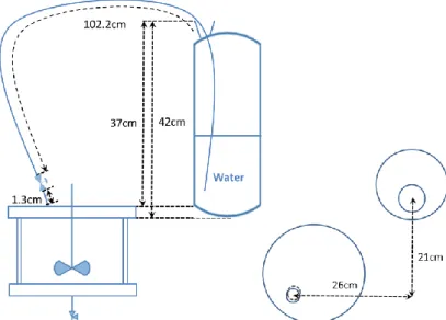
Figure II-5 Global planning of visualization reaction – Kiwi ... 67

Figure II-6 Position of the quench tank and corresponding relief line ... 68

Figure II-7 Swagelok Regulators – KBP Series: (a) outside view; (b) configuration ... 70

Figure II-8 Dynamic pressure versus static pressure ... 70

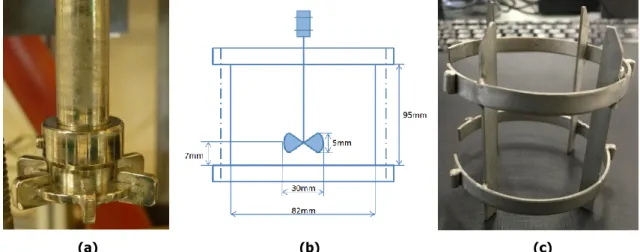
Figure II-9 Image of (a) stirrer; (b) configuration of the stirred reactor; (c) baffle ... 71

Figure II-10 Stirring mode and stirred flow pattern: (a) stirring without baffles; ... 71

Figure II-11 Power number calculation process ... 72

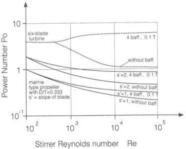
Figure II-12 Power number versus stirrer Reynolds number(Mersmann, 2001) ... 72

Figure II-13 Power curves (a) at different stirring rate; (b) at various viscosity ... 73

Figure II-14 Gas dispersion flow patterns (Jakobsen, 2008) ... 73

Figure II-15 Theoretical gas flow rate for the transition ... 74

Figure II-16 Recording temperature data ... 76

Figure II-17 Linear regressions ... 76

Figure II-18 T and P profile to closed reactor experiments ... 79

Figure II-19 (a) T P recording; (b) temperature increase rate ... 80

Figure II-20 Measurement of average void fraction ... 81

Figure II-21 VSP2 system configuration ... 82

Figure II-22 (a) Position of closed cell in heater; (b) close cell ... 83

Figure II-23 Water experiment results ... 84

Figure II-24 Comparison of water vapor pressure ... 84

Figure II-25 Comparison for two protocol: (a) Vapor pressure; (b) dT/dt profile ... 85

Figure II-26 VSP2 Similarity Vent-Screening Tool (a) Schema; (b) image ... 86

Figure II-27 Blowdown cell with ¼” vent line ... 87

Figure II-28 Orifice calibration results ... 88

Figure II-29 VSP2 simulation tool, blowdown experiment results ... 89

Figure II-30 Measurement noise (a) of temperature and (b) of pressure ... 90

Figure II-31 Adiabaticity: (a) one water experiment; (b) water experiment results ... 91

Figure II-32 Adiabaticity results after the runaway reaction ... 91

(20)

Figure II-34 Schema for a closed blowdown cell ... 93

Figure II-35 Phi factor evolution versus the fill level for closed and close blowdown cell ... 93

Figure II-36 UN 10L reactor (a) image; (b) schema ... 94

Figure II-37 Position of thermocouple in the glass vent line ... 94

Figure III-1 T and P evolutions and images during methanol boiling in Kiwi reactor. ... 102

Figure III-2 Temperature and pressure during an esterification experiment ... 103

Figure III-3 Images during an esterification boiling ... 104

Figure III-4 (a) Methanol boiling; (b) esterification runaway boiling ... 105

Figure III-5 (a) T and P evolutions for hot & cold wall; (b) T increase rate for hot & cold wall ... 106

Figure III-6 Average void fraction evolution ... 107

Figure III-7 Average void fraction against dT/dt ... 107

Figure III-8 (a) T and P evolutions for 3 [H2SO4]; (b) T increase rate for 3 [H2SO4] ... 108

Figure III-9 Average void fraction evolution ... 110

Figure III-10 Average void fraction (a) against dT/dt ; (b) against time ... 110

Figure III-11 T and P evolutions for 2 [H2SO4] (a); T increase rate for for 2 [H2SO4] (b) 111 Figure III-12 Average void fraction evolution ... 112

Figure III-13 Average void fraction against dT/dt ... 113

Figure III-14 T and P evolutions for 3 Pset (a); T increase rate for 3 Pset (b) ... 114

Figure III-15 Average void fraction against P with different Pset ... 115

Figure III-16 (a) T and P evolutions for 3 Pset; (b) P against T for 3 Pset ... 116

Figure III-17 Average void fraction against T (a) and P (b) with different Pset ... 118

Figure III-18 T and P evolutions for different µ (a); T increase rate for different µ (b) ... 119

Figure III-19 Flow pattern observation for non-viscous (a) and 86mPa.s (b) experiments ... 120

Figure III-20 Images during an esterification boiling at 87.2mPa.s ... 121

Figure III-21 Surface profile for two viscosity ... 123

Figure III-22 Evolution of the average level swell with different viscosity ... 123

Figure III-23 (a) T and P evolutions for different µ; (b) T increase rate for different µ ... 124

Figure III-24 Images during an esterification boiling at 30mPa.s ... 125

Figure III-25 Evolution of the average level swell with different viscosity ... 127

Figure III-26 T and P evolutions for different µ (a); T increase rate for different µ (b) ... 127

Figure III-27 Images during an esterification boiling at 375mPa.s ... 128

(21)

Figure III-29 (a) T and P evolutions for different stirring; (b) T increase rate for different

stirring ... 132

Figure III-30 Evolution of the average level swell ... 134

Figure III-31 Esterification runaway venting non-viscous system ... 137

Figure IV-1 Temperature increase rate for different concentrations of H2SO4. ... 151

Figure IV-2 Comparison between the model and VSP2 experiment ... 152

Figure IV-3 (a) jg,max for 5ppm [H2SO4] experiment, (b) temperature evolution ... 152

Figure IV-4 Sensitivity analysis ... 153

Figure IV-5 Sensitivity study (a) 1.9 x reaction rate; (2) 0.7 x liquid mass ... 154

Figure IV-6 jg,max of the experiment 350 mPa.s ... 154

Figure IV-7 jg,max calculation results from ᾱ and different churn turbulent flow pattern correlations ... 155

Figure IV-8 Sensitivity analyses for the three Correlations: (a) Ishii; (b) FAI Bubbly; (c) FAI CT. ... 156

Figure IV-9 Vapor superficial velocity Results for the unstirred experiments ... 156

Figure IV-10 jg,max [H2SO4]=5 ppm, Pset = 0.5barg: (a) versus ᾱ; (b) Accuracy ... 157

Figure IV-11 Vapor superficial velocity Results for the unstirred experiments ... 157

Figure IV-12 Vapor superficial velocity results for different stirring model... 158

Figure IV-13 Viscous and low reaction rate system ... 158

Figure IV-14 High reaction rate system at different viscosity ... 159

Figure IV-15 350 mPa.s experiment results (a) versus ᾱ, (b) comparison ... 159

Figure IV-16 Void fraction in bubbly flow (Zuber N. and Hench .J, 1962), cited in (Levy, 1999) ... 160

Figure IV-17 Flow pattern map with varying stirring mode and viscosity ... 161

Figure IV-18 Flow pattern map: non-viscosity experiments ... 162

Figure IV-19 Complexity of the runaway scenario ... 163

Figure 1 Comparison of the flow pattern and transition criteria (a) our study; (b) DIERS 171 Figure 2 Methodology ... 172

(22)

List of Tables

Table I-1 Different names according to different authors for the same flow regimes ... 24 Table I-2 Differences between a runaway flow and a large pipes flow ... 24 Table I-3 Flow pattern criteria (Fisher et al., 1993) ... 25 Table I-4 Observation of Bell and Morris ... 28 Table I-5 Different correlations for churn-turbulent flow ... 40 Table I-6 Different correlations for churn-turbulent flow ... 41 Table I-7 Different correlations ... 44 Table I-8 Parameters for different flow pattern ... 44 Table I-9 Equation for C0 ... 46

Table I-10 Correlations of u∞ ... 46

Table II-1 Comparison of chemical system ... 57 Table II-2 Proprieties of the chemicals ... 59 Table II-3 Parameters for each chemical ... 60 Table II-4 Parameters of the viscosity ... 60 Table II-5 Parameters for liquid heat capacity & enthalpy of vaporization ... 61 Table II-6 Surface tension measurement ... 63 Table II-7 Sensitivity study parameters ... 64 Table II-8 Chemical reference ... 64 Table II-9 Closed experiment GC results ... 65 Table II-10 Venting experiment results ... 65 Table II-11 Viscosity measurement for the mixture with PVP ... 66 Table II-12 Viscosity measurement for the mixture with PEO ... 66 Table II-13 Power requirement classification (Harnby, Edwards and Nienow, 2001) ... 72 Table II-14 Calculation results ... 76 Table II-15 Parameters for Antoine equation – water vapor pressure ... 83 Table II-16 VSP2 results for a closed cell and a closed blowdown cell ... 93 Table II-17 Mass for different cells ... 93 Table III-1 Information for respective image during methanol boiling ... 102 Table III-2 Condition of esterification experiment ... 103

(23)

Table III-3 Information for respective image during esterification runaway ... 104 Table III-4 Image comparison for cold wall and hot wall experiments ... 106 Table III-5 Information for respective image for different [H2SO4] ... 108

Table III-6 Image comparison for 3 [H2SO4] ... 109

Table III-7 Information for respective image for different [H2SO4] ... 111

Table III-8 Image comparison for 3 [H2SO4] ... 112

Table III-9 Mass loss at different [H2SO4] ... 113

Table III-10 Information for respective image for different Pset ... 114

Table III-11 Image comparison for 3 Pset with stirring (no baffles) ... 115

Table III-12 Image comparison for 3 Pset without stirring ... 117

Table III-13 Mass loss at different set pressure ... 118 Table III-14 Information for respective image ... 121 Table III-15 Image comparison for low viscosity low reaction rate condition ... 122 Table III-16 Information for respective image for different viscosity... 124 Table III-17 Information for respective image ... 125 Table III-18 Image comparison for low viscosity high reaction rate condition ... 126 Table III-19 Information for respective image for different viscosity... 127 Table III-20 Information for respective image ... 128 Table III-21 Image comparison for different viscosity at high reaction rate ... 129 Table III-22 Mass loss for different viscosity ... 130 Table III-23 Information for respective image for different stirring mode ... 132 Table III-24 Images from experiments ... 133 Table III-25 Images at the end of an esterification boiling at 350 mPa.s ... 135 Table IV-1 Reaction kinetic results for non-catalyzed system ... 150 Table IV-2 Some kinetic values in the literature ... 150 Table IV-3 Reaction kinetic results ... 151

(24)

General introduction

Runaway reactions are exothermic chemical reactions which would abruptly show a non-controlled increase in temperature and pressure. Some common causes that might lead to runaway reactions include cooling failure, incorrect charging, excessive heating, decomposition, contamination of reactants, loss of agitation and leak of heat transfer liquid into inside the reactor, etc. Such scenarios could make the reactor pressure much higher than the equipment maximal design pressure. To protect process vessels from catastrophic effects of an excessive overpressure and subsequent damage in the chemical industries, emergency relief systems (ERS) are frequently employed.

Several strategies have been developed to deal with the vent sizing of an ERS. These methodologies can range from a direct empirical scale-up, which is based on data from a small scale runaway reproduction, to exhaustive scientific studies of the physique chemistry and the venting dynamics coupled with complicated computer codes. The Design Institute for Emergency Relief System (DIERS) methods have been recognized as the best engineering practices for safe relief requirements.

Catastrophic results can be prevented even if an over-sizing or an unrealistically large ERS is designed. However, this substantially increases the cost of the emergency relief and release collection systems. The overestimation is usually due to the absence of analyses of the physical nature of the vent release. In this way, it is critical for the sizing an appropriate EMS to determine the composition of the venting flow, one-phase (gas or vapor) or two-phase (gas-liquid), under runaway conditions.

The phenomenon of level swell in the reactor during a runaway reaction, which means how the bubbles disengage from the liquid phase (disengagement model from DIERS Project Manual (Fisher et al., 1993)) is essential to the venting flow prediction.

In several computer codes, gas-liquid disengagement models are proposed. These models are correlations deduced from experiments in a bubble column system at stationary conditions which means that there is no void fraction variation in the height where the measurements are done. On the contrary, knowing the flow pattern in a reactor requires a quantitative knowledge of kinetics, thermodynamic, hydrodynamic

(25)

and even physical properties of the system during a runaway reaction. In summary, it is necessary to understand the disengagement, the flow pattern inside a reactor.

The final objective of this thesis is to develop a methodology to predict the nature of the vent release at industrial scale based on thermodynamic and physicochemical data of the reacting system, the size of the vent, its set pressure..., whatever reactive system is.

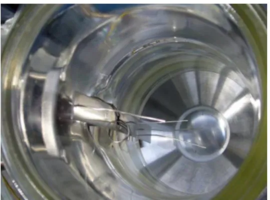
Inspired by the traditional gas-liquid flow pattern research in a bubble column and by the reported lab scale visualization experiments, a visualization tool was adapted from a glass reactor, in the Solvay laboratory Process & Product Safety in Lyon. This visual equipment, named Kiwi, permits to observe directly the bubble generation and the flow pattern to measure the level swell during a runaway reaction. The esterification between methanol and acetic anhydride, catalyzed by sulfuric acid, was chosen to be the reactive system. In the visualization reactor, a parametric study was carried out by changing the reactor wall temperature, the concentration of the catalyst (5 - 20 ppm) and therefore the reaction rate, the set pressure (0 – 1 barg), the viscosity1_{(1.6 – 375}

mPa.s) and the stirring mode. A camera was used to film the runaway scenario, and from the images, the average void fraction was measured.

At the same time, at Ecole des Mines de Saint-Etienne (EMSE), in SPIN center (Sciences des Processus Industriels et Naturels), a pseudo-adiabatic calorimeter (VSP2) was used to acquire the necessary thermodynamic data. Then a mass balance and an energy balance have been built-up to calculate the superficial vapor velocity (vapor flow rate/cross section area).

A flow pattern map for the studied reactive system has been plotted by using the measured average void fraction and the calculated superficial vapor velocity. Combined with the visual observation, the boundaries of the different flow patterns have been added.

This thesis consists on four main chapters. Chapter I aims at summarizing a bibliographic review focusing on (1) the disengagement flow pattern and (2) the disengagement model development, which gives an overview of the impact of the disengagement on the venting flow nature and the necessity of a deep study on this topic.

Chapter II introduces the reactive system, describes the experimental devices, the measurements, and the experimental protocol.

(26)

Then, Chapter III shows the experimental results: the recorded pressure and temperature, the bubble formation, the flow pattern analysis and the measurement of the average void fraction.

In order to compare experimental results with modeling, Chapter IV shows the superficial vapor velocity calculation from the average void fraction and from the energy balance. Furthermore, the construction of the flow pattern map is shown in this chapter.

(27)

(28)

Introduction générale

L’emballement d’une réaction signifie une perte de contrôle lors d’une réaction exothermique, qui par conséquent augmente brutalement la température et la pression dans une unité/réacteur. Les causes courantes qui pourraient conduire à telle situation sont, par exemple, une panne de refroidissement, une injection de réactifs absente, trop importante ou de composition chimique anormale, un chauffage excessif, une décomposition ou une contamination des réactifs, une perte d'agitation ou une fuite de liquide de transfert de chaleur à l'intérieur du réacteur, etc. Ces scénarios pourraient rendre la pression du réacteur beaucoup plus élevée que la pression maximale permise par l'équipement. Afin de protéger ces unités des effets catastrophiques d'une surpression et des dommages matériels et humains subséquents, des dispositifs d’évent de secours (ERS- emergency relief system) sont fréquemment utilisés.

Le dimensionnement des é vents de secours reste un challenge. Plusieurs méthodologies ont été développées allant de l’augmentation d'échelle à partir de données à petite échelle ou d’études exhaustives de la physico-chimique, de la dynamique d'évacuation, associées souvent à des modélisations compliqués. Les méthodes de l’Institut de Design pour les Système de secours d'urgence (DIERS) ont été reconnues comme une des meilleures approches pour le dimensionnement d’un évent de sécurité.

Les catastrophes peuvent être évités en utilisant un ERS bien dimensionné ou même surdimensionné. Cependant, un surdimensionnement peut augmenter considérablement le coût des systèmes de sécurité et de collecte des rejets. La surestimation est généralement due à l'absence de connaissance de la nature physique du rejet à la sortie de l’évent. De cette façon, il est essentiel de pouvoir déterminer la nature du rejet: monophasique (gaz ou vapeur) ou diphasique (gaz-liquide) pour un dimensionnement approprié d'un EMS en cas d’un emballement de réaction.

Le phénomène de gonflement du liquide dans le réacteur lors d'un emballement, dépend de la manière dont les bulles se désengagent de la phase liquide (modèle de désengagement du « DIERS Project Manuel » (Fisher et al., 1993)) et est essentielle à

(29)

Dans plusieurs softwares informatiques, des modèles de désengagement gaz-liquide sont intégrés. Ces modèles sont des corrélations déduites d’expériences des colonnes à bulle dans une zone d’étude stationnaire, ce qui signifie qu'il n'y a pas de variation de la fraction de vide dans la verticale où les mesures sont effectuées. Cependant, le fait de connaître le régime d'écoulement dans un réacteur nécessite une connaissance quantitative de la cinétique, des propriétés thermodynamiques, de l’hydrodynamique et de la physico-chimie du système réactif lors d'un emballement.

L'objectif ultime de cette thèse est de connaitre mieux le comportement de l’écoulement (désengagement) en cas d’un emballement de réaction et de développer une technique de caractérisation pour tout nouveau système chimique (réactif, solvant, concentration) qui permette de prédire la nature du rejet à l’évent (gazeuse ou diphasique) à l’échelle industrielle à partir d’un jeu minimal d’expériences à l’échelle du laboratoire, de données thermodynamiques ou physico-chimiques et d’informations sur l’installation industrielle (dimensions du réacteur, taille de l’évent, pression d’ouverture…).

Inspiré par l’étude du régime d’écoulement dans des colonnes à bulle et par les expériences de visualisation à l'échelle du laboratoire, un outil de visualisation fut construit à partir d'un réacteur en verre de 0,5 l, dans le laboratoire « Solvay Process & Product Safety » à Lyon. Cet équipement de visualisation, appelé « Kiwi », permet d'observer directement la génération de bulles et le régime d'écoulement, à fin de mesurer le gonflement du liquide lors d'un emballement de réaction. L'estérification entre le méthanol et l'anhydride acétique, catalysée par l'acide sulfurique, fut choisie comme système modèle pour cette étude. Dans le réacteur de visualisation, une étude paramétrique fut effectuée en modifiant la température de la paroi du réacteur, la concentration du catalyseur (5 à 20 ppm), donc la vitesse de réaction, la pression d’ouverture (0 - 1 barg), la viscosité (1,6 - 375 mPa.s) et le mode de l’agitation. Une caméra permet de filmer le scénario de l’emballement et, à partir des images, de mesurer la fraction de vide moyenne.

En parallèle, à l'Ecole des Mines de Saint-Etienne (EMSE), dans le centre SPIN (Sciences des Processus Industriels et Naturels), un calorimètre pseudo-adiabatique (VSP2) fut utilisé pour acquérir les données thermodynamiques du système. Ensuite, un bilan massique ainsi qu’un bilan énergétique ont été construits pour calculer la vitesse superficielle de la vapeur (débit de vapeur / section).

Une carte du régime d'écoulement pour le système réactif fut tracée en utilisant la fraction de vide moyenne mesurée et la vitesse de vapeur superficielle calculée à partir des bilans. Combinés aux observations, les frontières des différents régimes d'écoulement ont été ajoutées.

(30)

Cette thèse se compose de quatre chapitres principaux. Le chapitre I est un état de l’art sur (1) les modèles de désengagement et (2) le développement de ces modèles, donnant un aperçu de l'impact du désengagement sur la nature du rejet et mettant en exergue l’importance de l’étude approfondie de ce sujet.

Le chapitre II présente le système réactif, décrit les dispositifs expérimentaux, les mesures et les protocoles de manips utilisés.

Ensuite, le chapitre III montre les résultats expérimentaux de la visualisation: la pression et la température enregistrées, la formation de bulles, l'analyse du régime d'écoulement et la mesure de la fraction de vide moyenne.

Afin de comparer les résultats expérimentaux avec la modélisation, le chapitre IV montre le calcul de la vitesse superficielle de vapeur à partir de la fraction de vide moyenne et des bilans. En outre, la construction de la carte des régimes est expliquée dans ce chapitre.

(31)

(32)

State of the Art

Chapter I

The objective of this chapter is to give a global view of the vent sizing and of the disengagement model.

The first section gives a general introduction into the runaway reaction and emergency relief systems.

The outline of the DIERS vent sizing proposal will be presented in section 2. The hydrodynamic regime, so the concept of “disengagement” will be pointed out.

Section 3 will discuss the disengagement flow pattern and the transition criteria. In this section, the flow pattern definition for the vent sizing purpose and for the traditional bubble column research will be summarized and compared between them. The precise and visualization experiments done in the past will also be shown.

In section 4 the disengagement model will be presented in order to answer 3 questions: What is the disengagement model? How did it was built? What are the application conditions and limitations?

(33)

(34)

Runaway Reaction and Emergency Relief System

I.1.

Definition of a thermal runaway reaction

I.1.1.

In the chemical industry, exothermic chemical reactions can lead to a thermal runaway if the heat generation exceeds the heat remove. The runaway reaction is usually characterized by an exponential and uncontrolled increase in temperature. Thus, runaway reactions may lead to:

 an increase in the chemical reaction rate;

 the appearance of undesired reactions because of the specific kinetics under runaway conditions leading to the formation of uncontrolled byproducts and also in some cases decomposition can occur;

 a pressure increase during the runaway reaction when liquid components vaporize or noncondensable gas is produced. The overpressure under runaway conditions can make grave equipment ruptures or even an explosion.

Some common causes of a runaway reaction due to a problem with cooling are usually: failure of cooling water due to the electrical or mechanical failure of pumps, choking of the condenser used for cooling, high cooling water temperature or insufficient cooling water pressure. Runaway reaction may also be observed from other failures, such as incorrect charging sequence, agitator failure, contamination of reactants, too fast additions quick, removal of volatile solvent, etc. Apart from the occurrence of a runaway reaction during a chemical conversion process, self-heating during storage, transport or unit operations like drying can lead to the thermal instability of materials, and result in undesirable events.

An approach to deal with hazards that may accompany runaway reactions is the analysis of safe operation conditions and process monitoring as prevention of runaway in reactions. By this way, runaway reactions can be identified and analyzed but cannot be eliminated. In order to prevent consequences of a runaway reaction, an inhibitor, injection of a coolant and a pressure relief system can be used. In general, in the case of prevention approach, a full evaluation of the process hazards must be carried out, before the design of the protective system. Emergency vents are often present on the reactors for the relief of runaway reactions. Because the vented stream may be toxic, corrosive, and at high temperature and so on, simply having a vent on a reactor can be not enough, and some equipment must be added to flow the discharge from the vent device into the needed treatment units.

(35)

Emergency relief system

I.1.2.

An emergency relief system (ERS) is mainly installed in a reactor, a chemical plant or a storage tank where a thermal runaway reaction can occur, to prevent the pressure vessels from damaging or exploding. An emergency relief system is also called final safety device which discharges a certain amount of fluid and controls the pressure under runaway emergency. It acts as the final safety solution, and it is activated once all other security devices and mechanisms have failed.

They need to be designed for the worst possible case in order to guarantee that the release area is sufficient to evacuate the system in every possible situation. There are mainly two types of emergency relief vents: pressure relief valve and bursting disc (rupture disc). They work differently, and each one presents its own benefits and limitations.

Pressure relief valve

I.1.2.1.

The pressure relief valve is a type of valve that automatically actuates as soon as the vessel pressure is higher than the valve working pressure in order to discharge the fluid. When the pressure decreases to the desired value, the valve closes again.

The pressure relief valve can close after an operation, keeping the rest of the mixture inside the vessel. In general, the safety valve needs to be protected against viscous products, highly corrosive mediums, etc. Moreover, the safety valve needs to be away from harsh operating conditions, which could have an impact on the good functionality of the safety device.

Figure I-1 Pressure relief valve

Bursting discs (Rupture Discs)

I.1.2.2.

A bursting disc, also known as a rupture disc, is designed as a non-reclosing pressure relief device that protects a pressure vessel, equipment or system from overpressure risk after the rupture of bursting disc. A rupture has a one-time-use membrane which provides a more instant response in system pressure, usually more effective than a pressure relief valve, but once the disc has ruptured, it will not reseal. Using bursting discs is leak-tightness and has a higher cost compared to pressure relief valves.

(36)

Figure I-2 Bursting disc before and after a rupture

Relief vent sizing: DIERS method

I.2.

The vent sizing aims to determine the vent size that is able to limit the abnormal pressure increase inside a reactor or a storage tank in the worst case during a runaway reaction. The vent must be large enough to allow sufficient pressure relief by sufficient flow rate in order to protect the vessels. Conversely, an oversizing vent can be very costly for the industry because of the cost of the oversized vent, vent line, corresponding treatment and recycle system.

Introduction to the DIERS vent sizing method

I.2.1.

Formed in 1976 by a consortium of 29 companies, the Design Institute for Emergency Relief Systems (DIERS) is dedicated to the development of methods to the design of emergency relief systems in order to handle runaway reactions (Fisher et al., 1993). DIERS became a huge group in 1985 with over 200 companies (75 percent domestic and 25 percent international).

The Purpose of the DIERS group is to reduce the frequency, the severity and the consequences of the pressure making accidents, and to develop new techniques which will improve the design of emergency relief systems. Both small-scale (32 L) and large-scale (2200 L) blowdown experiments for nonreactive and reactive systems have been performed in order to understand the mechanism and construct the simulation method.

DIERS spent about $1.6 million in research works to acquire the experimental data and to document the vent sizing methods for two-phase vapor-liquid flow. They were involved in the investigation of the two-phase vapor-liquid disengagement dynamics and the hydrodynamics of the emergency relief systems.

The venting flow nature: one or two phase flow has a direct impact on the vent area. In order to have an appropriate sizing of the vent device is necessary to know the venting flow nature. The nature of the venting flow depends on the chemical system behavior inside the reactor. During the venting scenario, the chemical-physical proprieties, the thermodynamics and the hydrodynamics change. Furthermore, the choice of the relief vent, the flow hydrodynamics thought the relief vent and in the

(37)

pipeline also have some influence on the venting flow nature.

Figure I-3 Venting flow nature

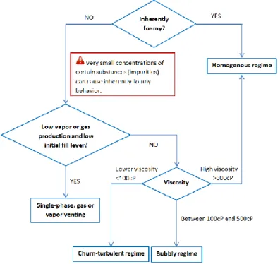
In the following section, the four behaviors inside the reactor will be presented according to the DIERS method.

Thermodynamic characterization of the system

I.2.2.

In order to design a relief system, it is essential to identify how the pressure is generated in the system. There are three types of systems:

 Vapor systems, in which the pressure increase is a consequence of the evaporation of the reactants and/or products in the vessel, because of the temperature rise due to the thermal/reaction runaway.

 Gassy systems, in which the pressure is generated by non-condensable gases produced by the chemical reaction.

 Hybrid systems, in which the pressure increases due to both the noncondensable gas generation and the vapor pressure with the temperature rise.

For a vapor system, the relief system needs to remove the vapor efficiently, to remain a constant temperature and therefore a constant pressure. Such a pressure relief system is referred to as a tempered system. Generally, the reaction rate does not increase again after relief. However, in some cases, the reaction rate can continue to increase at this constant temperature and pressure, as the influence of the composition change during the conversion of the reaction, the mass loss due to the venting, sometimes, a condition change, such as pH change or autocatalysis.

A gassy system is “untempered” because the removal of the gas will not have an influence on the temperature rise and on the reaction rate. The relief system needs to be designed to the corresponding to the maximum gas generation rate.

A hybrid system is “non-tempered” when the vapor pressure is less than 10 % of the total pressure.

Thermodynamic Hydrodynamic Chemical kinetics

Relief vent

(38)

The classification of the different reaction systems for the relief vent sizing is given in Fig I-4.

Figure I-4 Different thermodynamic systems

Characterization of the system: disengagement models

I.2.3.

The knowledge of the composition of the venting flow is essential for the vent sizing. A one phase gas venting needs a smaller vent area compared to a two-phase venting, and the proportion of the gas phase in a two-phase venting can influence the vent sizing. In general, the evacuation of the gas is more efficient for the depressurization. “Disengagement” describes the capacity for the bubble to slip from the liquid bulk, which is related to the relationship between the gas/vapor and the liquid in the reactor during a runaway reaction.

For a two-phase vapor-liquid system, the boiling surface can rise to the level of an emergency relief vent if enough bubbles hold up the liquid in a vessel. In some systems, it is easier for the gas to slip from the liquid; therefore the surface rise of the liquid is small. Sometimes, the liquid phase can entrap the bubbles. In this case, if enough bubbles are entrapped, the liquid surface reaches the level of the emergency relief vent, and a two-phase flow can occur. The rise of the liquid can be measured and is referred to as the “level swell”.

A disengagement flow model was proposed in 1983 (Fauske H & Associates, 1983) considering three types of disengagement flow pattern:

 Homogeneous flow

In this case, there is no movement between the bubble and the liquid phase which means that there is zero gas disengagement. If the mixture surface reaches the level of the relief vent, the average void fraction is equal to the void fraction in the vessel. Because no bubbles leave the liquid, this flow pattern leads to a maximum level swell.

Runaway reaction

Hybrid system Gassy system

Vapor system

Untempered system Tempered system

(39)

 Bubbly flow

The bubble disengagement flow pattern in the vessel is limited with a continuous liquid phase with discrete bubbles. The bubbly flow assumes that the bubble generation is uniform in the bulk. The homogenous flow can be considered as the extreme limiting case of the bubbly flow (Robert D’Alessandro, 2004).

 Churn-turbulent flow

This flow pattern is characterized by a substantial release of gas through the liquid surface where the liquid phase is continuous with coalesced vapor regions of increasing size relative to the bubbly flow. The churn-turbulent flow also assumes a uniform bubble generation throughout the liquid. The size of the bubbles in the bulk and at the liquid surface is heterogeneous and will oscillate the surface when this one is attained.

 Other models

In 1993, the “no boiling region model” (Fisher et al., 1993) was proposed. This model is a modified churn-turbulent flow model. In a high reactor, the generation of the bubbles cannot occur near the bottom of the reactor. Thus a non-boiling height above the bottom of the reactor vessel is formed and can be estimated from a balance between hydrostatic heat effects and recirculation effects.

Besides this, it was also defined a “complete vapor-liquid disengagement model”, when all the vapor is formed at or near the liquid surface or that the vapor ascension velocity is larger enough so that the swelled liquid does not reach the relief vent.

In 2006, Fauske proposed “the wall boiling model” (Fauske, 2006) for the H2O2

decomposition. In this case, the vapor is generated on the lateral reactor wall, in a very similar manner to what happens in the case of fire exposure. The disengagement is 10 times more efficient than in a Churn-turbulent flow pattern. This model does not concern a uniform vapor generation.

The disengagement models have been developed to predict the venting flow nature of a reactive system. Once the disengagement flow pattern is defined, the level swell and the gas flow rate can be calculated by the related flow pattern correlations. When the level swell does not reach the vent line, a one-phase vapor/gas vent flow appears; when the level swell is higher than the reactor height, a two-phase flow can appear. At this time, the vapor proportion can be calculated from different flow pattern correlations.

(40)

Because the disengagement models are indispensable and direct for the venting flow nature prediction, this study will be focused on the disengagement models. These models will be thus developed in detail in sections I.3 and I.4.

Chemical kinetics – adiabatic calorimeter experiment

I.2.4.

In an industrial reactor, a large quantity of reactants is used. During a runaway situation, the heat exchange between the reactive mass and its surrounding is limited and generally negligible compared to the released heat by the reaction. Thus the reactor is considered under adiabatic conditions.

One of the strategies to understand the runaway reaction is data acquisition from direct sizing method which simulates the worst case conditions in an industrial reactor in a pseudo-adiabatic or adiabatic calorimeter to obtain the thermal runaway reaction rate.

Such an adiabatic calorimeter can measure the pressure and temperature behavior in a test cell (in glass or in metal) during the experiment. The heat exchange is controlled by the heater outside the test cell. The reaction released heat will totally heat the reactive system and the test cell. One small part of the energy is used to heat the test cell, so a correction can be used to ensure adiabaticity. Furthermore, the pressure inside the test cell can be balanced by an outside pressure regulation.

The different acquisition commercial devices are the Accelerating Rate Calorimeter (ARCTM_{), Vent Sizing Package II (VSP2), Advanced Reactive System Screening Tool}

(ARSST), Automatic Pressure-Tracking Adiabatic Calorimeter (APTAC TM_{), PHI-TEC} TM

and DEWAR Calorimeter.

During this Ph.D. experimental study, the VSP2 will be used as the calorimeter tool.

Vent sizing calculation outline

I.2.5.

The purpose of the DIERS proposal is to provide to the user’s group a simple and safe way to size the vent area.

The general design involves a series of steps; the model is based on the mass and energy balances for the reaction. In this section, an outline will be given to describe in brief the vent sizing calculation. These steps are the following:

1) Screen the different scenarios and identify the “worst case” (requiring the largest relief vent area).

(41)

when the runaway attains its maximum. This maximum should be defined in function of the reactive system nature: tempered or non-tempered. This reaction rate can be the measurement by the adiabatic calorimeter mentioned in Section I.2.4.

3) Choose an appropriate disengagement model.

The venting flow nature and the discharge flow rate are determined by the disengagement models in function of the disengagement flow pattern: homogeneous, bubbly and churn-turbulent. In the case of a two-phase vent flow, the mass fraction or volumetric fraction of the gas phase can be evaluated by different correlations. Special cautions need to be made in the case of, the presence of few impurities which can change the flow behavior inside the reactor totally.

4) Vent area calculation.

For the calculation, the reaction rate is measured by an adiabatic calorimeter. The experiments in the calorimeter are carried out in the same or at similar conditions in the reactor.

Flow pattern inside a reactor and the transition criteria

I.3.

The disengagement was first studied and reported in the DIERS Report FAI/83-27(Fauske H & Associates, 1983) for the top discharge system with non-viscous and non-foaming fluids, then in several papers among which Leung 87, Project Manual, Shepperd & Morris, and D’Alessandro 2004 (Leung, 1987; Fisher et al., 1993; Sheppard and Morris, 1995; Robert D’Alessandro, 2004). Typical examples of such systems are water, Refrigerant 11 (Trichlorofluoromethane), 12 (Dichlorodifluoromethane), and other pure organics such as ethyl benzene.

One description of the disengagement was given by the DIERS Project Manual (Fisher

et al., 1993): during the gas boiling or gas-sparged through the volume of liquid, the rising bubbles cause the liquid to swell. Individual bubbles are able to rise through the liquid with a velocity that is dependent on the buoyancy and surface tension and retarded by the viscosity, the foamy character of the fluid, and the interactions with other bubbles. The ability of bubbles to escape from the liquid is called “disengagement”.

D’Alessandro defined total disengagement, partial disengagement and no disengagement or homogeneous venting (Robert D’Alessandro, 2004). If the bubbles slip from the mixture efficiently to retain the surface of swelled liquid below the top of the vessel, single-phase vapor venting occurs. This is referred as complete disengagement. If the ability of bubbles to slip is not enough, the swelled liquid

(42)

reaches the top of the vessel and the two-phase venting occurs, which is referred to as

partial disengagement. If the bubbles cannot slip from the mixture, there is no disengagement at all, and the homogeneous two-phase venting takes place.

The heat generation due to the exothermic chemical reaction leads to a vapor generation inside the reactive mixture. The vapor generation rate is generally considered to be uniform over the reactive mixture. If gas disengagement occurs, void fraction  is generally larger in the higher parts of the vessel contents. The magnitude of this void fraction gradient depends on the vessel flow pattern (more pronounced for churn-turbulent bubble flow than for bubbly flow). The level of the mixture can reach the top of the vessel (2- vent flow) or not (1- vapor vent flow). Solving the problem of the flow at the vent thus involves being able to determine the quality of the flow at the vent inlet xi from pieces of information at the global reactor scale (total vapor

generation rate, vessel flow regime).

The objective of this thesis is to predict the nature of the venting flow (one phase gas or two phases gas-liquid) during a runaway reaction. For that, the two-phase flow pattern in the reaction will directly influence the venting flow nature and the fraction of vapor within the venting mixture. As mentioned in section I.2.3, different disengagement flow patterns have been proposed. This study is focused on the three more general ones: homogeneous, bubbly and churn-turbulent flow pattern.

Figure I-5 Dramatic effect of allowing for overpressure (Fauske, 2006)

The homogeneous and bubbly flow have very similar behavior. Section I.3.1 considers the bubble generation issues: bulk (homogeneous) or nucleation boiling (heterogeneous). The definition, the transition and some influence of the flow pattern are discussed in section I.3.2. It is shown in section I.3.3 the visualization experiments for a different system, and section I.3.4 introduces the homogeneous flow.

Bulk boiling or nucleation boiling in industrial reactors?

I.3.1.

(43)

boiling (uniform bubbles generation in the volume) for modeling disengagement during a blowdown at approximately constant pressure for a reactive system. However, homogeneous bubble nucleation (a consequence of superheat) is difficult to obtain experimentally, because interfacial nucleation is almost always available in a container. Are those two points compatible or contradictory?

Blander and Katz (Blander and Katz, 1975) gave a review covering the homogeneous (bulk) and heterogeneous (surface or interface) bubble nucleation. They gave some theoretical and experimental demonstrations.

In the case of organic liquids, experiments with homogeneous bubble nucleation were described as follows:

Small droplets of a volatile liquid were introduced into the bottom of a column of a denser immiscible liquid medium. The immiscible medium is heated non-uniformly so that it is hotter at the top. As the droplets slowly rise, they get hotter and hotter until they attain the limit of superheat, they nucleate (they vaporize) and they explode. Media used for a successful experiment are sulfuric acid, glycerin, ethylene glycol, chloride-water mixture, and ammonia-water mixtures.

For water boiling, the attempts have been made with superheated water droplets in silicone oil. The nucleation occurred between 250 °C and 275 °C. Furthermore, they have tried the superheat of several mixtures using the droplet technique. If the components have the similar boiling points, the liquid boils with a fairly sharp explosive report. For mixtures with relative volatile components in an involatile solvent, the volatile component boils at a higher temperature. Adding solvent can also change the character of the phenomenon: the bubble size, the amplitude of boiling.

Their conclusion is that homogeneous nucleation can occur when liquid is superheated until 88 % - 90 % of their critical temperature under some conditions:

 a necessary condition: the heated liquid is not in contact with a vapor phase,  a sufficient but not necessary condition: the liquid wets (has a zero contact

angle with) all surfaces which are in contact.

These conditions can be met when the liquid is completely enclosed by a high surface tension material with a smooth surface, for example, a glass or another involatile liquid.

The bubble nucleation is linked closely to the reactor wall condition. Glass is generally used (Grolmes and Fauske, 1974): “Glass (Pyrex) was chosen because its surface was smooth enough to suppress any undesirable heterogeneous nucleation and made visualization possible” (Simões-Moreira and Shepherd, 1999). “In order to simulate the

(44)

effect of metallic container walls on the inception and propagation of evaporation waves, metallic inserts were arranged in the experiment tubes.” (Hahne and Barthau, 2000).

In fact, covering the free surface with glycerol (probably for suppressing free surface boiling) permitted a slow depressurization to the extent that the fluid readily sustained liquid superheat in excess of 95 °C before releasing through nucleation at some wall cavity site (Grolmes and Fauske, 1974). However, this is not possible in a reactor.

For a non-reactive system, the heat comes from an external heater. For an exothermic chemical reaction system, the liquid mixture can boil if there are at least one volatile species. The external heater can provide the necessary energy to start the reactions, then, the reactions release also heat. The vapor bubble nucleation obeys the same principle as a non-reactive system. Heterogeneous (nucleation) boiling is thus much more probable than homogeneous (bulk) boiling when heat comes from a chemical reaction, exactly as it is for other sources of boiling.

In the beaker, the jacketed reactor and other equipment in lab scale, the pilot scale reactor or the industrial reactors, there is always vaporization, so the liquid phase is in direct contact with its vapor phase. The scratched surface of the reactor, the stirrer, the heater will foster a heterogeneous bubble nucleation. In general, the superheating in a reactor is very small compared to 90 % of the critical temperature. Thus, homogeneous bubble nucleation is extremely difficult to obtain.

Flow pattern definition and transition criteria

I.3.2.

More recent studies like: Boesmans (Boesmans and Berghmans, 1995), Cumber(Cumber, 2002) and Colomer & Rogers (Colomer and Rogers, 2006), tried to improve the correlations for a runaway reaction inspired by the works of Ishii and al. (Ishii, 1977; Kaichiro and Ishii, 1984). Another article, such as Hibiki (Hibiki and Ishii, 2003) and Schlegel (Schlegel et al., 2013) extended the study to large pipes. This section aims to present:

 The different definitions/classifications of the flow patterns.  The transition criteria.

Types of flow patterns

I.3.2.1.

In the literature, several different terms were sometimes used to describe the same flow pattern. In order to better distinguish the different flow pattern and study the transition criteria, this part summarizes the various terms and clarifies the definitions of the flow patterns.

(45)

Many studies about flow pattern deal with small pipes, where the bubble size can be of the same order of magnitude as the diameter of the pipe.

Figure I-6 One traditional flow regimes in small pipes (Ashfaq Shaikh and Muthanna H. Al-Dahhan, 2007)

Fig I-6 shows a series of traditional flow regimes in small pipes, where slug flow exists between the bubble flow and churn flow. However, the “true slug flow” (with Taylor bubbles of the diameter of the pipe) cannot exist in large vessels. Levy (Levy, 1999) notes that “for a smaller channel size, the churn-turbulent flow would take the form of slug flow”. This also means the flow patterns depends on the pipe size. The size of the bubbles in a reactor is generally small compared to the vessel diameter. Naturally, this literature review is restricted to what happens in “large pipes”.

Each chemical system has its own chemical-physical propriety, so the notion of “large pipe” or the minimum pipe diameter in order to be a large pipe is not always the same for the different systems. The DH* is defined as the dimensionless hydraulic diameter:

𝐷_𝐻∗ ₌ 𝐷𝐻

√𝜎 𝑔∆𝜌⁄ Eq I-1

When the DH* is greater than 30 – 40, the formation of the Taylor bubbles, which

occupy the entire cross section, is no longer possible.

In large pipes, the surface instability leads to the breakup of the large “Taylor” bubbles. Such “reformed” small bubbles have a highly distorted surface (Shen et al., 2014). This results in a flow more varied and complex in the aspect of hydrodynamics. The prediction of the flow structure with the turbulence is more difficult.

Zuber & Hench 1962 (Zuber N. and Hench .J, 1962) (cited by (Levy, 1999)) is a frequently cited experimental source in the literature about disengagement flow patterns. They observed a 10 cm x 10 cm large “batch” system and db < 1 cm. They

Caractérisation de la nature physique du rejet d’un évent en cas d’emballement de réaction : étude du modèle de désengagement

HAL Id: tel-01844260

https://tel.archives-ouvertes.fr/tel-01844260

Caractérisation de la nature physique du rejet d’un

évent en cas d’emballement de réaction : étude du

modèle de désengagement

Jie Xu

To cite this version:

THESE de DOCTORAT DE L’UNIVERSITE DE LYON

opérée au sein de

l’Ecole des Mines de Saint-Etienne

Ecole Doctorale

N° 488

Sciences, Ingénierie, Santé

Spécialité de doctorat

Soutenue publiquement le 09/10/2017, par :

Jie XU

Caractérisation de la nature physique

du rejet d’un évent dans le cas d’un

emballement de réaction : étude du

modèle de désengagement

Devant le jury composé de :

To

my beloved parents

and

Be not afraid of life,

Believe that life is worth living,

And your belief will help create the fact.

From William James

Acknowledgement

Contents

List of Symbols

Glossary

List of Figures

List of Tables

General introduction

Introduction générale

State of the Art

Chapter I

Runaway Reaction and Emergency Relief System

I.1.

Definition of a thermal runaway reaction

I.1.1.

Emergency relief system

I.1.2.

Pressure relief valve

I.1.2.1.

Bursting discs (Rupture Discs)

I.1.2.2.

Relief vent sizing: DIERS method

I.2.

Introduction to the DIERS vent sizing method

I.2.1.

Thermodynamic characterization of the system

I.2.2.

Characterization of the system: disengagement models

I.2.3.

Chemical kinetics – adiabatic calorimeter experiment

I.2.4.

Vent sizing calculation outline

I.2.5.

Flow pattern inside a reactor and the transition criteria

I.3.

Bulk boiling or nucleation boiling in industrial reactors?

I.3.1.

Flow pattern definition and transition criteria

I.3.2.

Types of flow patterns

I.3.2.1.