To link to this article:
DOI: 10.1002/2016JA022797
URL:
http://dx.doi.org/10.1002/2016JA022797
Any correspondence concerning this service should be sent to the repository
administrator:
[email protected]
O
pen
A
rchive
T
OULOUSE
A
rchive
O
uverte (
OATAO
)
OATAO is an open access repository that collects the work of Toulouse researchers and
makes it freely available over the web where possible.
This is a publisher-deposited version published in:
http://oatao.univ-toulouse.fr/
Eprints ID: 16109
To cite this version:
Garcia, Raphael and Bruinsma, Sean and Massarweh, Lotfi
and Eelco, Doornbos Medium-scale gravity wave activity in the thermosphere
inferred from GOCE data. (2016) Journal of Geophysical Research: Space
Physics, vol. 121 (n° 8). pp. 8089-8102. ISSN 2169-9402
Medium-scale gravity wave activity in the thermosphere
inferred from GOCE data
Raphael F. Garcia1, Sean Bruinsma2, Lotfi Massarweh3, and Eelco Doornbos3
1Institut Supérieur de l’Aéronautique et de l’Espace, ISAE-SUPAERO, Toulouse, France,2Department of Terrestrial and
Planetary Geodesy, CNES, Toulouse, France,3Faculty of Aerospace Engineering, TU Delft, Delft, Netherlands
Abstract
This study is focused on the effect of solar flux conditions on the dynamics of gravity waves (GWs) in the thermosphere. Air density and crosswind in situ estimates from the Gravity Field and Steady-State Ocean Circulation Explorer (GOCE) accelerometers are analyzed for the whole mission duration. The analysis is performed in the Fourier spectral domain averaging spectral results over periods of 2 months close to solstices. A new GW marker (called C3f) is introduced here to characterize GWs activity under low,
medium, and high solar flux conditions, showing a clear solar damping effect on GW activity. Most GW signal is found in a spectral range above 8 mHz in GOCE data, meaning a maximum horizontal wavelength of around 1000 km. The level of GW activity at GOCE altitude is strongly decreasing with increasing solar flux. Furthermore, a shift in the dominant frequency with solar flux conditions has been noted, leading to larger horizontal wavelengths (from 200 to 500 km) during high solar flux conditions. The correlation between air density variability and GW marker allows to identify most of the large-amplitude perturbations below 67∘ latitudes as due to GWs. The influence of correlated error sources, between air density and crosswinds, is discussed. Consistency of the spectral domain results is verified in the time domain with a global mapping of high-frequency air density perturbations along the GOCE orbit. This analysis shows a clear dependence with geomagnetic latitude with strong perturbations at magnetic poles and an extension to lower latitudes favored by low solar activity conditions. These results are consistent with previous Challenging Minisatellite Payload (CHAMP) data analysis and with general circulation models.
1. Introduction
The gravity waves (GWs) propagating in the atmosphere/ionosphere system play a key role for energy transfer along the vertical direction [Vadas et al., 2009] and from pole to the equator.
GWs observed in the thermosphere originate in the lower atmosphere [Fritts and Alexander, 2003; Vadas and
Fritts, 2006; Vadas, 2007] as well as in the auroral and polar thermosphere [Richmond, 1978]. The auroral GWs,
which are the result of sudden energy deposition in the auroral zones (a ring-shaped zone at 60∘ –85∘ mag-netic latitude), have a large amplitude and wavelengths larger than 1000 km. Consequently, they are the easiest to observe. This highly variable and unpredictable energy input is predominantly in the form of Joule heating, which causes rapid and decidedly local density enhancements. Mass, momentum, and energy are redistributed, sometimes down to the equator, through a global circulation system. Several papers have pre-sented detailed investigations of Challenging Minisatellite Payload (CHAMP) GW activity on various scales [Bruinsma and Forbes, 2007, 2008, 2009]. Medium-scale GWs (horizontal wavelengths≤1000 km) are gener-ally assumed to be generated by energy inputs coming from the lower atmosphere [Yi˘git and Medvedev, 2010;
Miyoshi et al., 2014] or by ocean/atmosphere coupling phenomena [Artru et al., 2005; Garcia et al., 2014; Godin et al., 2015].
Such GWs are usually observed through the electron density perturbations induced by their pass in the iono-spheric layers [Hocke and Schlegel, 1996; Afraimovich et al., 2000; Liu et al., 2006; Occhipinti et al., 2006; Rolland
et al., 2010; Galvan et al., 2011] or through airglow variations [Hickey et al., 2010; Makela et al., 2011; Fukushima et al., 2012; Paulino et al., 2016].
However, the advent of several Low Earth Orbit (LEO) space missions dedicated to the mapping of Earth’s gravity field (CHAMP, Gravity Recovery and Climate Experiment (GRACE), and Gravity Field and Steady-State Ocean Circulation Explorer (GOCE)) recently allowed in situ observations of neutral density perturbations
RESEARCH ARTICLE
10.1002/2016JA022797
Key Points:
• Detection, characterization, and global mapping of the gravity waves (GWs) along the GOCE orbit • More GWs at short horizontal
wavelengths are observed in low than high solar flux conditions
• Space/time variations of GW activity are consistent with previous results based on satellite data and with GCMs
Supporting Information: • Supporting Information S1 Correspondence to: R. F. Garcia, [email protected] Citation:
Garcia, R. F., S. Bruinsma, L. Massarweh, and E. Doornbos (2016), Medium-scale gravity wave activity in the thermosphere inferred from GOCE data, J. Geophys. Res. Space Physics,
121, doi:10.1002/2016JA022797.
Received 5 APR 2016 Accepted 30 JUL 2016
Accepted article online 5 AUG 2016
©2016. American Geophysical Union. All Rights Reserved.
induced by GWs in the thermosphere. A detailed global climatology of medium-scale thermospheric GW activity observed by CHAMP is given in Park et al. [2014].
The objective of this study is to characterize the medium-scale GWs in the thermosphere (wavelength, amplitude, climatology, and variations with solar flux), using neutral densities and winds derived from thruster and accelerometer measurements performed by GOCE (Gravity Field and Steady-State Ocean Circulation Explorer) mission. First, the GOCE data set is introduced, focusing on the relation between wave’s physical parameters and observations. Then, we present data selection and some spectral estimators to detect and characterize GW trains and justify the validity of the analysis with a synthetic example. Next, the results of spectral analysis are presented, and variations of GW characteristics with latitude, season, and solar flux are discussed. The global mapping of high-frequency air density perturbations at GOCE altitude is shown in section 5, allowing to extend our analysis to high-latitude regions. Finally, we conclude and present directions for future studies.
2. GOCE Data Set
GOCE satellite moves in a quasi-polar orbit (nearly Sun synchronous with 97.5∘ inclination) at an almost con-stant altitude of around 270 km, through an ion thruster for drag compensation [Romanazzo et al., 2011]. GOCE accelerometer data are sampled at 0.2 Hz, while the ion thruster force is sampled at 0.1 Hz. Nongravitational accelerations of the satellite are known within 2 × 10⁻¹²m/s2[Floberghagen et al., 2011].
The air density and crosswinds data sets are retrieved by combining data of accelerometers and ion thruster (used for drag compensation). The deviation between observed and modeled accelerations allows also to compute the air density and crosswinds in the thermosphere with a relative error smaller than 2% [Doornbos
et al., 2010]. The crosswinds can be expressed in a S/C (spacecraft) body frame (VXalong the main GOCE dimen-sion approximately along track, VYcross satellite direction, and VZcompleting the right-hand system) or in
a local frame (VCNnorthward direction, VCEeastward direction, VUPupward direction). Thanks to the precise AOCS/DFACS control (Attitude and Orbit Control System/Drag-Free and Attitude Control System), the S/C X axis is almost parallel to the orbital motion and the roll axis is mostly orientated in the along-track direction [Romanazzo et al., 2011].
Parameters used in this study are the two components of the crosswind felt by GOCE, VUPand VY(mostly
zonal due to the quasi-polar orbit), and the relative air density variations Γ =𝜌HP∕𝜌LP, ratio between the high- and low-frequency components of the air density (cutoff at 640 s or 1.56 mHz using a fourth-order Butterworth filter). Due to a high orbital velocity (∼7750 m/s) compared to GW propagation velocity, our data set is essentially capturing the horizontal structure of GWs with a certain wavelength that can be calculated (in first approximation) taking into account the doppler effect as follow:
fobs≈ fGW+𝜅 ⋅ V𝜅 ⋅ V𝜅 ⋅ VGGG 2𝜋 = fGW+ VZ G 𝜆Z +V X Gcos(𝜃) 𝜆h (1) with fobsthe observed frequency in GOCE data, fGWthe intrinsic GW frequency,𝜅𝜅𝜅 =
[ 2𝜋 cos(𝜃) 𝜆h , 2𝜋 sin(𝜃) 𝜆h , 2𝜋 𝜆Z ] the wave number vector, VVVGGGthe GOCE orbital velocity vector, and𝜃 the angle between the GOCE orbit and the
GW propagation direction in the local horizontal plane. Considering GOCE velocity parameters (VX
G ≈ 7750 m/s and V Z
G ≈ 20 m/s) even in a worst-case scenario for
which we have a large intrinsic frequency and a small vertical wavelength (fGW = 2 mHz,𝜆Z ≈ 30 km, and 𝜆h≈ 500 km), the above equation can still be approximated by
fobs≈ V X Gcos(𝜃) 𝜆h = V X G 𝜆X (2) So the frequency of signals observed in GOCE data is directly related to the projection of the horizontal wavefront along the GOCE orbit direction. Note that𝜆X, the wavelength deduced from the frequency of
per-turbations in GOCE data, provides an overestimate of GW horizontal wavelength (𝜆X ≥ 𝜆h). The horizontal
wavelength is properly estimated only for waves propagating along GOCE track.
As a consequence of the above approximation, the gravity wave period cannot be resolved from GOCE data set.
Table 1. Main Parameters Under Different Solar Flux Conditions (Low, Medium, and High) for Both Seasonal Time Slots (May–June and November–December)a Passes
Period Flux Level Year Flux Range (sfu) MeanF10.7 MeanKp Midlatitude (North) Equatorial Midlatitude (South)
Low 2010 60→ 80 73.25 ± 3.38 1.795 ± 0.872 1763 1789 1785 May–Jun Medium 2011 80→ 110 95.90 ± 8.97 1.840 ± 0.876 1674 1691 1693 High 2012 110→ 190 121.03 ± 14.46 1.898 ± 0.811 1486 1505 1503 Low 2010 60→ 90 83.46 ± 4.54 0.898 ± 0.671 1720 1756 1756 Nov–Dec Medium 2012 90→ 130 114.57 ± 14.60 0.996 ± 0.802 1546 1573 1571 High 2011 130→ 190 147.13 ± 15.17 0.965 ± 0.628 1724 1744 1743 aFor each data set: the selected year, the flux range used, the mean and standard deviation ofF
10.7(daily solar flux) andKp(daily geomagnetic index), and the number of passes per latitude range. Note that during the GOCE mission (2009–2013) theF10.7ranged from 60 to 190 solar flux units.
3. Analysis Method
3.1. Data Set Selection and Splitting
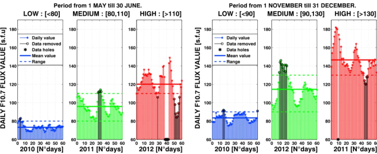
In order to distinguish between effects due to latitude variations from other atmospheric conditions, the data set has been separated in three different latitude zones (equatorial ±23∘ and midlatitudes north/south ±23∘ till ±67∘). Polar regions are excluded because strong short-period wind variations in these regions are due to the rotation of background wind relative to GOCE track, and not to GWs. The splitting of the data leads to time windows of size around 640–650 s (approximately one eighth of the orbital revolution) for each zone. Averages are computed over 2 months in order to obtain a sufficient number of passes and to ensure a reliable statistical result while keeping approximately the same atmospheric conditions relative to a given season. Two different time slots are selected in May–June and November–December because they present a low number of data gaps and they correspond to different mean solar fluxes for different years of the GOCE mission. These time slots are representative of the two solstices. Variations of solar fluxes and magnetic Kp index for the various years in these two times slots are provided in Table 1.
Figure 1 presents the daily F10.7distribution for the selected time periods, with F10.7relative ranges and mean
value and with data removed as described above.
As background context, we need to take into account that during the entire GOCE mission (2009–2013) the
F10.7ranged from 60 to 190 (sfu) with a mean value of 101.35 ± 27.36, meaning that the overall comparison is based on a period with a low to medium solar activity.
Our data set does not contain geomagnetic storms.
Figure 1. Values of daily solar flux (F10.7) for the two seasonal time slots: (left) May–June and (right) November– December, for the various years. In each subfigure, mean value (continuous line), boundaries (dashed line), data removed (black bars), and GOCE data gaps (black stars) are also shown. Daily solar data are provided by NOAA, Space Weather Prediction Center.
Figure 2. (top row) Air density perturbations in the horizontal plane for the three monochromatic synthetic wavefields. GOCE track at 96.7∘inclination (magenta line) and north direction (black arrow) are also indicated. (bottom row) From left to right, Amplitude Spectral Density (ASD) forVUP, Magnitude Squared Coherence (MSC) betweenVUPandVY, and
theC3f index for the synthetic data set given in Figure 3. 3.2. Spectral Analysis
The spectral analysis of GOCE data corresponding to passes in the different latitude bins was performed with three different spectral estimators. Then average values are computed for the selected 2 month periods. First, the Welch Amplitude Spectral Density (ASD) is estimated on 64 data points (at 0.1 Hz sampling rate), dividing the entire window size into eight sections with a 50% overlap. Each section is tapered by a Hamming window using the pwelch MATLAB function with standard settings [Welch, 1967]. A linear trend is removed from original data for each pass, in order to remove low-frequency variations. ASDs are estimated in the 2 to 50 mHz frequency range.
Second, the Magnitude Squared Coherence (MSC) between two of the three GOCE observables is computed with an algorithm similar to the one described above. The MSC is the spectral equivalent of the correlation coefficient. It is defined as
MSC[X,Y]= |⟨X|Y⟩| 2
⟨X|Y⟩ ⋅ ⟨X|Y⟩ (3)
with⟨X|X⟩ and ⟨Y|Y⟩ the power spectral densities of signals X, Y and ⟨X|Y⟩ the cross power spectral density. MSC ranges from 0 (no correlation at a given frequency) to 1 (perfect correlation at a given frequency). Finally, from the MSC computed for the three couples of observables, we define a new index C3
f as follows: C3 f = 3 √ |MSC[ ̇Γ,VUP]| × |MSC[ ̇Γ,VY]| × |MSC[VY,VUP]| (4)
where ̇Γ is the time derivative of Γ in GOCE data.
C3
fparameter ranges from 0 to 1. Zero value means that at least two of the three observables are uncorrelated,
whereas one value means that the three parameters are completely correlated. This parameter is a spectral equivalent of the time domain C3index defined by Garcia et al. [2014]. It is expected to provide values close to 1 for data bins and frequencies corresponding to GW crossings by GOCE.
Finally, for each zone and each time slot, we obtain an N-set of spectral curves, where N is the number of full passes (with at least 64 data points) that we are considering in the 2 month period selected. From this set, an average and an error estimate on this average are computed for each parameter (ASD, MSC, and C3
f) at each
frequency in the spectral range from 2 to 50 mHz.
3.3. Synthetic Example: Superposition of Three Gravity Waves in GOCE Data
We present a synthetic example under the hypothesis of quasi-monochromatic GWs propagating in the ther-mosphere. Three synthetic gravity wave trains are created following Nappo [2002]. These waves are assumed to propagate in a thermosphere without background wind, with N2= 10−4rad2/s2and an atmospheric scale
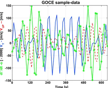
Figure 3. Synthetic GOCE observations for a satellite pass over the superposition of three GW trains, as described in Figure 2. Realistic measurement noise is added to the synthetic data both in time and space.
height of 43.5 km. The directions of propagation, wavelengths, and frequencies are provided in the titles of panels of Figure 2. The amplitudes of synthetic VYand ̇Γ signals are computed according to wave parameters and propagation direction relative to GOCE orbit assuming the same wave amplitude of 30 m/s for VUPsignal. Gaussian noises of standard deviation 1%, 2 m/s, and 5 m/s are added respectively to Γ, VY, and VUPsignals before reproducing the spectral analysis, and the starting phases are chosen randomly.
The simulated GOCE data set mixing the three GWs is shown in Figure 3 in time domain. From this plot, it is clear that the mix of different wavelengths projected along the GOCE orbit does not allow a visual identification of the wave trains.
An example of analysis performed for this synthetic case is given in Figure 2 (bottom row), with the ASD of
VUP, the MSC between VUPandVY, and the C3f marker.
The different GW synthetic wavelengths are producing clear peaks in the spectral domain for MSCs and the
C3
f marker. Note that these peak frequencies are not corresponding to the peak of the spectral power of the
signal, demonstrating that C3
f marker is independent of signal amplitude.
This synthetic example clearly demonstrates our ability to infer, in the spectral domain, the interference between different GW trains which is not possible in the time domain.
4. Results
4.1. Amplitude Spectral Density (ASD) In Figure 4, the average ASDs for the ̇Γ = dΓ
dt = d dt (𝜌 HP 𝜌LP )
are presented for the selected 2 month periods and for the three latitude ranges, each line presenting results corresponding to various years with different solar flux conditions. Solar flux, magnetic index Kp, and statistical parameters for these computations are pre-sented in Table 1. Due to the time derivative applied to the Γ parameter and to the detrending process, the long-wavelength variations multiple of orbit frequency are completely removed and high-frequency content is enhanced. For all periods and latitude ranges, a similar relation with solar activity is observed, with signal energy increasing with decreasing solar flux, in agreement with observations based on CHAMP data [Bruinsma
and Forbes, 2008]. The average ASDs present a peak of signal energy in the 8–50 mHz frequency range, and
the frequency of this peak is decreasing with increasing solar flux energy.
Examples of averaged ASD for cross-track and vertical winds along the GOCE orbit are presented in Figure 5 for midlatitudes north zone during the selected 2 month periods at various solar flux conditions. The variations observed in this latitude range are representative of the ones observed in the two other latitude ranges (not shown).
The cross-track wind presents much more energy at low frequencies than at high frequencies due to long-wavelength variations along the orbit induced by the variations of thermosphere zonal winds as a
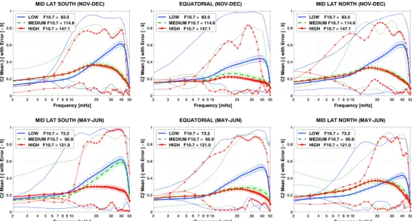
Figure 4. (top row) Average Amplitude Spectral Densities (ASDs) of the time derivative ofΓin the November–December seasonal time slot. From left to right, the results are presented for the three different latitude ranges: midlatitudes south (−67∘to−23∘), equatorial (−23∘to 23∘), and midlatitudes north (23∘to 67∘). On each panel, three different solar flux conditions are presented: low (blue plain line), medium (green dashed line), and high (red plain line with dots). (bottom row) Same as Figure 4 (top row) for the May–June seasonal time frame. Details on the data set can be found in Table 1.
Figure 5. Average Amplitude Spectral Density (ASD) in the November–December seasonal time slot for (top left)VYand (top right)VUPobservables and for different solar flux conditions: low (blue plain line), medium (green dashed line), and high (red plain line with dots). (bottom row) Same as Figure 5 (top row) for the May–June seasonal time frame.
Figure 6. For the November–December seasonal time slot in the equatorial latitude range, (top left) Average Magnitude Square Coherence betweenVUPandVY, (top middle) betweendΓ
dt andVY, and (top right) between dΓ
dt andVUP. (bottom row) Same as Figure 6 (top row) for the May–June seasonal time slot also in the equatorial latitude range.
function of latitude. The vertical wind presents also more energy at low frequencies that could also be ascribed to background wind latitude variations. However, it exhibits a much flatter spectrum than the cross-track winds.
As already observed for relative density variations, the spectral power of these two components of wind in the range 8–50 mHz increases with a decreasing solar flux. These variations due to different solar fluxes are ascribed to a varying GW power, as demonstrated below.
4.2. Magnitude Squared Coherence (MSC)
The average MSC for all combinations of possible parameters is presented in Figure 6 for the equatorial latitude range. Variations observed in this zone are similar to the ones observed in the other two latitude ranges (not shown). For all combinations of parameters, the average MSCs present a peak of correlation in the 8–50 mHz range, and both the maximum value and the peak frequency are increasing with decreasing solar flux energy. Because these parameters are expected to be correlated when GOCE is crossing a GW front, these computations demonstrate that correlation peaks above 8 mHz in GOCE data can be ascribed to GWs. 4.3. The C3
f Index for Detection and Characterization of Gravity Waves Activity As discussed above, C3
f is a marker of GW perturbations measured along the GOCE orbit. The advantage of
this new parameter compared to the C3index computed in the time domain by Garcia et al. [2014] is that it allows to characterize the frequency content of GW perturbations observed in the GOCE data. In addition, we can use equation (2) to relate the dominant frequency observed in GOCE data to the maximum horizontal wavelength of GWs.
As observed in Figure 7, the average C3
f presents a peak in the 8–50 mHz range corresponding to GWs of
horizontal wavelengths smaller than 1000 km, consistent with the fact that GWs of wavelengths larger than 1000 km are rare in the thermosphere [Miyoshi et al., 2014]. The Nyquist frequency of GOCE data set limits our investigations to horizontal wavelengths larger than 150 km. However, the average C3
f values at Nyquist
frequency are low, suggesting that most of the range of GW horizontal wavelengths is captured by GOCE data, consistent with the fact that propagation conditions do not favor short-wavelength GWs [Fritts and
Vadas, 2008].
For all latitude zones and for the two periods considered, the average C3
f peak amplitudes and frequencies
are increasing with decreasing solar flux. The increase of average C3
f amplitude in the 8–50 mHz range is
Figure 7. (top row) AverageC3
f values (lines with error bars) and single-pass values corresponding to maximum/
minimumC3
f energy in the 8–50 mHz range (lines without error bars) for the November–December seasonal time slot.
From left to right, the results are presented for the three different latitude ranges: midlatitudes south (−67∘to−23∘), equatorial (−23∘to 23∘), and midlatitudes north (23∘to 67∘). In each panel, three different solar flux conditions are presented: low (blue plain line), medium (green dashed line), and high (red plain line with dots). (bottom row) Same as Figure 7 (top row) for the May–June seasonal time frame. Details on the data set can be found in table 1.
of average C3
f peak frequency reflects the presence of GW with decreasing wavelengths with increasing solar
flux conditions, going from average maximum wavelengths of 200 km (40 mHz) at low solar flux (F10.7≈ 80) to 1000 km at high solar flux (F10.7≈ 120).
Finally, the average C3
f values and the peak frequencies in the equatorial region are generally lower than for
midlatitude regions during the same time periods, suggesting that the waves are propagating mainly from the pole to the equator and that they are damped along their path during their propagation [Vadas, 2007]. Figure 7 also presents estimates of C3
f along single passes corresponding to minimum and maximum C
3
f
energy in the 8–50 mHz range for a given latitude zone. These curves show that GW activity can strongly vary from one pass to another and that the C3
f parameter has a significant standard deviation on top of the
average values presented above. The presence of different local maximums for a given pass may be due to the interference of different GW fronts at different horizontal wavelengths and/or orientations relative to GOCE obit.
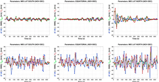
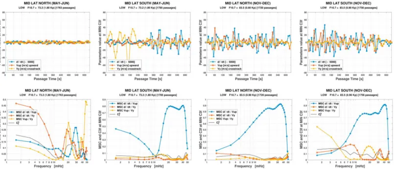
The time domain data of passes with maximum C3
f energy in the 8–50 mHz range are presented in figure 8 for
the November–December period at high and low solar flux conditions. The wave amplitude is clearly lower at high solar flux conditions than at low solar flux conditions. The absence of long-period signals (f ≤ 8 mHz) is also clear in this plot. Finally, the dominant period appears also to be larger at high solar flux conditions than at low solar flux. So the trends observed statistically on the spectra are visible on individual passes for which GWs are detected.
4.4. Air Density Perturbations: Gravity Waves or Thermosphere Dynamics?
The previous sections described a marker of the presence of gravity waves in GOCE data and its variability with solar flux, latitude, and season. In order to infer if the air density variability observed by GOCE in the 8–50 mHz frequency range is dominated by gravity waves or by thermosphere dynamics, we plotted in Figure 9 the stan-dard deviation of Γ as a function of maximum value of C3
fin this frequency range for each orbit arc analyzed.
These plots clearly show the strong dependence of air density variability with solar flux conditions previously described. These results also reveal a clear correlation between relative air density standard deviation and maximum value of C3
f parameter which is expected for the variability due to the presence of gravity waves.
This correlation is more pronounced for data close to the equator than at midlatitudes, demonstrating that more than 80% of the large-amplitude variability observed close to the equator is due to the presence of
Figure 8. (top row) For high solar flux conditions in November–December seasonal time slot, time domain plots of the three physical parameters ̇Γ(blue line),VUP(green line), andVY(red line) for the particular GOCE pass with maximumCf3
energy in the 8–50 mHz range and in the different latitude ranges: midlatitudes south (left), equatorial (middle), and midlatitudes north (right). (bottom row) Same as Figure 8 (top row) for low solar flux conditions in November– December seasonal time slot.
gravity waves. At midlatitudes and for low solar flux conditions, about 30% of GOCE orbit arcs having rela-tive air density standard deviations larger than 0.1 (10%) present a maximum C3
f value lower than 0.7 in the
8–50 mHz frequency range. Consequently, the air density variability along these arcs cannot be ascribed to gravity waves from GOCE data. We suggest that it is due to air density variations induced by the dynamics of the polar thermosphere which extend to lower latitudes during low solar flux conditions, because this vari-ability is much less pronounced close to the equator. But we cannot exclude that a part of this varivari-ability is due to gravity waves propagating almost exactly along the GOCE orbit track because our method cannot detect these waves due to the absence of signal along the cross-track direction. Overall, Figure 9 demonstrates that more than 60% of the air density variability observed at latitudes lower than 67∘ can be ascribed to the propagation of gravity waves.
4.5. Error Analysis
Our method of GW detection and characterization relies on the correlations between air density and cross-wind variations within the GW. However, such correlations may also occur due to errors in the air drag modeling. In particular, the error on the mounting angles of GOCE electric thruster induces a mapping of drag due to air density into crosswinds.
Figure 9. Scatterplots of relative air density (Γ) standard deviation as a function of maximumC3
f value in the 8–50 mHz frequency range for all GOCE orbit arcs
analyzed in low (in black) and high (in red) solar flux conditions. From left to right, equatorial region in May–June period, midlatitudes in May–June period, equatorial region in November–December period, and midlatitudes in November–December period. Error level on relative air density estimates (1%) is also indicated.
We can split the air density (𝜌) and the cross track wind (Vc= V
Yor VUP) measured by GOCE into four different terms: 𝜌d=𝜌0+𝜌HF+𝜌GW+ N𝜌=𝜌p+ N𝜌 (5) Vc d= V c 0+ V c HF+ V c GW+ NVc+𝛼𝜌p (6)
with terms indicated by subscripts 0, HF, and GW corresponding respectively to the physical effects of long-wavelength variations along GOCE orbit, high-frequency variations induced by thermosphere dynam-ics, and high-frequency variations induced by GWs. The noise terms N𝜌and NVcare assumed to be instrument
white noise. The term𝛼𝜌prepresents the correlated error between the crosswind and the air density with𝛼 a
constant parameter depending only on thruster misalignment angles. Because of GW polarization, the cross-track wind component Vc
GWcan be written [Garcia et al., 2014]:
VGWc =𝛽(𝜔)ΓGW (7)
with𝛽(𝜔) being nonzero only in the frequency (e.g., horizontal wavelength) range corresponding to GWs. Our analysis filters out the long-term variations𝜌0and V0cand uses the time derivative of relative air density fluctuations ( ̇Γ).
After some straightforward computations and a Fourier transform, we obtain
̇Γ = i𝜔(ΓHF+ ΓGW+N𝜌
𝜌0 )
(8)
Vc= VHFc +𝛽(𝜔)ΓGW+ NVc+𝛼𝜌0(ΓHF+ ΓGW) (9)
with ̇Γ and Vcthe parameters used in the statistical analysis presented above.
If we assume that instrument noises NVcand N𝜌are not correlated, and that air density and wind variations
induced by high-frequency thermosphere dynamics and GWs are not correlated between themselves, we obtain the following relation for the cross power spectral density:
⟨ ̇Γ|Vc⟩ = i𝜔𝛼𝜌
0⋅ ⟨ΓHF|ΓHF⟩ + i𝜔(𝛼𝜌0+𝛽(𝜔)) ⋅ ⟨ΓGW|ΓGW⟩ (10) This equation demonstrates that the correlated error between winds and air density variations (scaled by𝛼 for a given crosswind direction) increases the cross power density and consequently the MSC between our parameters.
From this equation, and taking into account the scaling of MSC by power spectral densities, we expect strong MSC values induced by correlated errors between the parameters in the following situation:
1. GW signal is smaller than the other high-frequency variations induced by thermosphere dynamics: ⟨ΓGW|ΓGW⟩ ≪ ⟨ΓHF|ΓHF⟩.
2. Signal-to-noise ratio of air density variations is larger than 1:N 2
𝜌 𝜌2
0 ≪ ⟨ΓHF|ΓHF⟩ 3. Correlated error on cross-track wind is larger than noise: N2
Vc≪ 𝛼2𝜌20⟨ΓHF|ΓHF⟩. The first condition corresponds to the curves with lowest values of C3
f in Figure 7. The other two
condi-tions are favored by the presence of strong high-frequency background variacondi-tions of air density and winds, encountered mainly at midlatitudes during low solar flux conditions.
Figure 10 presents MSCs computed for cases corresponding to the above conditions. The data correspond-ing to minimum C3
f in Figure 7 were extracted for midlatitudes at low solar flux conditions. Among the four
examples provided, the sample data for north midlatitudes in May–June 2010 period (on the left) have a low signal level and do not ensure that the signal-to-noise ratio is good enough to detect correlated errors. For the other three examples the vertical crosswind (VUP) is clearly correlated with high-frequency air density pertur-bations ( ̇Γ), even in the absence of GW signal (low C3
f values). Other examples presenting low C
3
f values with
large-amplitude signals in other solar flux conditions (not shown) also show large values of MSC[ ̇Γ,V UP]. These observations suggest that the vertical crosswind presents correlated error sources with air density per-turbations. This was also suggested by the observation in Figure 6 of average values of MSC between these
Figure 10. (top row) Time domain plots of the three physical parameters ̇Γ(blue line),VUP(red line), andVY(yellow line). (bottom row) Corresponding values of MSCs between the parameters andC3f. The extracted data are corresponding to lowestCf3curves presented in Figure 7. From left to right, midlatitudes north and south for May–June period and midlatitudes north and south for November–December period in low solar flux conditions.
two parameters larger than 0.2 for frequencies lower than 8 mHz, outside the GW frequency/wavelength range. Fortunately, such a correlated error is not observed between horizontal cross-track wind (VY) and air
density perturbations ( ̇Γ), so the analysis given above is not strongly affected because it is supported mainly by
C3
f values. The correlated error source between VUPand Γ will be revised in future reprocessing of GOCE data.
5. Global Mapping of High-Frequency Perturbations at GOCE Altitude
The spectral analysis presented above allows to clearly identify most of the high-frequency signals recorded above 8 mHz in GOCE data as due to GW signals. However, it does not provide precise spatial distribution information. In this section, we present a global mapping analysis that allows to display the spatial distribution of the GWs.
5.1. Data and Methods
The space/time splitting and selection of data sets match exactly the one used for solar flux analysis presented in the previous sections. In order to isolate and observe GW activity, the data are high-pass filtered above 8 mHz.
The GOCE orbit allows full Earth coverage with 1∘ resolution in less than 1 month. The latitude/longitude space is split in bins of size 4∘ latitude by 10∘ longitude, ensuring always more than 200 data points in each bin during the selected 2 month periods. For each bin, the averages and standard deviations of high-pass filtered parameters Γ, VUP, and VYare computed over the 2 month periods. We checked that the average values are
close to zero (not shown), or much smaller than standard deviations, due to the high-pass filtering. 5.2. Global Mapping of High-Frequency Relative Density Perturbations
We present only the results for relative density perturbations (Γ), because cross-track and vertical winds present strong small-scale variations close to the poles that are due to thermosphere wind pattern and not to GW perturbations.
Figure 11 presents the standard deviations of high-pass filtered Γ over the globe at GOCE altitude. Because these signals correspond to frequencies above 8 mHz, we expect it to represent mainly GWs of wavelengths below 1000 km. Major activity is observed in polar regions, especially near geomagnetic poles indicated by magenta squares. However, the GOCE orbit inclination does not allow a full coverage up to the poles
Figure 11. Standard deviation of theΓparameter (relative air density perturbations, color bar) along the GOCE orbit, high-pass filtered above 8 mHz, as a function of latitude and longitude for the (top row) November–December and (bottom row) May–June seasonal time slots and for different solar flux conditions: low (left), medium (middle), and high (right). North and south geomagnetic poles are indicated by magenta squares.
(above 85∘ latitude). The high-frequency energy along the orbit is clearly higher during low solar flux condi-tions than during high solar flux. The perturbacondi-tions, extending from poles to equator, are asymmetric during May–June time period with highest energy in the Southern Hemisphere.
Despite the slight differences in data processing and significant differences in altitude range, our results are quite similar to the results obtained by Park et al. [2014] from CHAMP satellite data which are presented in a similar form in their Figures 2 and 3. They also observed decreasing GW activity with increasing solar flux, asymmetrical hemispherical patterns during June solstice, and a high level of air density variability close to magnetic poles.
6. Discussion
The statistical variations of both the dominant frequency of GW signal in GOCE data and the number of GW events, from high to low when increasing the solar flux, suggest an increase in atmospheric damp-ing/attenuation of the waves during their propagation in the atmosphere when increasing solar flux [Bruinsma
and Forbes, 2008; Yi˘git and Medvedev, 2010]. These observations at GOCE altitude will allow to better
under-stand the relative influence of winds, Brunt-Vaisala frequency, and attenuation parameter variations with solar flux through their direct effects on GW propagation [Yi˘git and Medvedev, 2015].
Our space/time variations of high-frequency relative density variations agree with the results of Park et al. [2014] obtained from CHAMP satellite data at higher altitudes. This agreement suggests that the GWs observed by GOCE continue to propagate upward to the 300–400 km altitude range. The amplitudes of the relative density variations observed by GOCE at minimum solar flux are significantly larger (maximum 6%) than the ones observed by CHAMP (maximum 1.8%) which suggests again that the GWs are significantly attenuated during their vertical propagation from ∼270 km to ∼350 km altitude.
In addition, there is a striking similarity between the results obtained for low solar flux conditions in Figure 11 and the simulation results by Miyoshi et al. [2014] presented in their Figures 6(b) and 12(a) and obtained under approximately the same conditions (300 km altitude, solstice averages). In particular, the high-frequency air density perturbations in the Southern Hemisphere below −50∘ latitude and the maxima of perturbations close to the geomagnetic poles are corresponding to regions where these authors predict a high GW energy. They explain their results by the focusing of upward propagating GWs by the winds in the mesosphere at 60∘ latitude and around the pole for GWs created in the troposphere by both convective activity and mountain waves.
7. Conclusion
In this study we present an analysis performed for different 2 month seasonal periods (shifted by 6 months, in proximity of the two solstices). The analysis in the spectral domain is based on three main parameters, sampled in situ by GOCE satellite, dΓ∕dt, VUP, and VY. The spectral characteristics of these signals are
deter-mined through their Amplitude Spectral Density, the Magnitude Squared Coherence, and a new frequency domain parameter C3
f, for arcs of 640 s in the midlatitudes and equatorial regions. Despite some correlated
errors between vertical wind and air density variations, our analysis demonstrates that GW signals are domi-nating in GOCE data above 8 mHz. This frequency range corresponds to horizontal wavelengths smaller than 1000 km. Strong variations with solar flux conditions are observed, with more GW detections and shorter wavelengths during low solar flux conditions than during high solar activity. Moreover, the number of GWs detected is decreasing with latitude. In order to infer further this spatial trend, maps of high-frequency relative density variations are presented for the selected 2 month periods. In low solar flux conditions, the activity is stronger in the winter hemisphere than in the summer hemisphere. However, the picture is asymmetric with a Southern Hemisphere more active than the Northern Hemisphere. Whatever the solar activity conditions, the geomagnetic poles are the regions presenting the most air density perturbations.
During low solar flux conditions part of the dynamics of the polar thermosphere may extend to lower latitudes, because a significant part of the air density variability during low solar flux cannot be explained by gravity waves propagating in the thermosphere.
Our results are in overall agreement with previous analysis of CHAMP data [Park et al., 2014] and with GCM simulation studies [Yi˘git and Medvedev, 2010; Miyoshi et al., 2014] that predict variations of thermospheric GW activity with solar flux induced by the related variations of their propagation conditions from the troposphere to the thermosphere. The comparison with simulations by Miyoshi et al. [2014], performed for low solar activ-ity at the same season and approximately the same altitude, reveals the same spatial patterns and a similar north/south asymmetry.
This study enhances the great interest of GOCE data for modeling of GW activity in the atmosphere/ thermosphere. Future reprocessing of GOCE data will reduce correlated errors between parameters, allowing to infer more precisely the GW characteristics.
References
Afraimovich, E. L., E. A. Kosogorov, L. A. Leonovich, K. S. Palamartchouk, N. P. Perevalova, and O. M. Pirog (2000), Determining parameters of large-scale traveling ionospheric disturbances of auroral origin using GPS-arrays, J. Atmos. Sol. Terr. Phys., 62, 553–565, doi:10.1016/S1364-6826(00)00011-0.
Artru, J., V. Ducic, H. Kanamori, P. Lognonné, and M. Murakami (2005), Ionospheric detection of gravity waves induced by tsunamis,
Geophys. J. Int., 160, 840–848.
Bruinsma, S. L., and J. M. Forbes (2007), Global observation of traveling atmospheric disturbances (TADs) in the thermosphere, Geophys. Res.
Lett., 34, L14103, doi:10.1029/2007GL030243.
Bruinsma, S. L., and J. M. Forbes (2008), Medium- to large-scale density variability as observed by CHAMP, Space Weather, 6, S08002, doi:10.1029/2008SW000411.
Bruinsma, S. L., and J. M. Forbes (2009), Properties of traveling atmospheric disturbances (TADs) inferred from CHAMP accelerometer observations, Adv. Space Res., 43, 369–376, doi:10.1016/j.asr.2008.10.031.
Doornbos, E., J. Van Den Ijssel, H. Luehr, M. Foerster, and G. Koppenwallner (2010), Neutral density and crosswind determination from arbitrarily oriented multiaxis accelerometers on satellites, J. Spacecr. Rockets, 47, 580–589, doi:10.2514/1.48114.
Floberghagen, R., M. Fehringer, D. Lamarre, D. Muzi, B. Frommknecht, C. Steiger, J. Piñeiro, and A. da Costa (2011), Mission design, operation and exploitation of the gravity field and steady-state ocean circulation explorer mission, J. Geod., 85, 749–758, doi:10.1007/s00190-011-0498-3.
Fritts, D. C., and M. J. Alexander (2003), Gravity wave dynamics and effects in the middle atmosphere, Rev. Geophys., 41(1), 1003, doi:10.1029/2001RG000106.
Fritts, D. C., and S. L. Vadas (2008), Gravity wave penetration into the thermosphere: Sensitivity to solar cycle variations and mean winds,
Ann. Geophys., 26, 3841–3861, doi:10.5194/angeo-26-3841-2008.
Fukushima, D., K. Shiokawa, Y. Otsuka, and T. Ogawa (2012), Observation of equatorial nighttime medium-scale traveling ionospheric disturbances in 630-nm airglow images over 7 years, J. Geophys. Res., 117, A10324, doi:10.1029/2012JA017758.
Galvan, D. A., A. Komjathy, M. P. Hickey, and A. J. Mannucci (2011), The 2009 Samoa and 2010 Chile tsunamis as observed in the ionosphere using GPS total electron content, J. Geophys. Res., 116, A06318, doi:10.1029/2010JA016204.
Garcia, R. F., E. Doornbos, S. Bruinsma, and H. Hebert (2014), Atmospheric gravity waves due to the Tohoku-Oki tsunami observed in the thermosphere by GOCE, J. Geophys. Res. Atmos., 119, 4498–4506, doi:10.1002/2013JD021120.
Godin, O. A., N. A. Zabotin, and T. W. Bullett (2015), Acoustic-gravity waves in the atmosphere generated by infragravity waves in the ocean,
Earth Planets Space, 67, 47, doi:10.1186/s40623-015-0212-4.
Hickey, M. P., G. Schubert, and R. L. Walterscheid (2010), Atmospheric airglow fluctuations due to a tsunami-driven gravity wave disturbance, J. Geophys. Res., 115, A06308, doi:10.1029/2009JA014977.
Hocke, K., and K. Schlegel (1996), A review of atmospheric gravity waves and travelling ionospheric disturbances: 1982–1995,
Ann. Geophys., 14, 917–940, doi:10.1007/s00585-996-0917-6.
Acknowledgments
We are grateful to two anonymous reviewers for improving this study by their constructive comments. This study was funded by CNES (Centre National d’Etudes Spatiale) through space research projects. Data are available through the GOCE+ Thermospheric Data archive at the ESA website: https:// earth.esa.int/web/guest/missions/ esa-operational-missions/goce/goce-thermospheric-data.
Liu, J. Y., Y. B. Tsai, S. W. Chen, C. P. Lee, Y. C. Chen, H. Y. Yen, W. Y. Chang, and C. Liu (2006), Giant ionospheric disturbances excited by the M9.3 Sumatra earthquake of 26 December 2004, Geophys. Res. Lett., 33, L02103, doi:10.1029/2005GL023963.
Makela, J. J., et al. (2011), Imaging and modeling the ionospheric airglow response over Hawaii to the tsunami generated by the Tohoku earthquake of 11 March 2011, Geophys. Res. Lett., 38, L00G02, doi:10.1029/2011GL047860.
Miyoshi, Y., H. Fujiwara, H. Jin, and H. Shinagawa (2014), A global view of gravity waves in the thermosphere simulated by a general circulation model, J. Geophys. Res. Space Physics, 119, 5807–5820, doi:10.1002/2014JA019848.
Nappo, C. (2002), An introduction to atmospheric gravity waves, 276 pp.
Occhipinti, G., P. Lognonné, E. Kherani, and H. Hébert (2006), Three-dimensional waveform modeling of ionospheric signature induced by the 2004 Sumatra tsunami, Geophys. Res. Lett., 33, L20104, doi:10.1029/2006GL026865.
Park, J., H. Lühr, C. Lee, Y. H. Kim, G. Jee, and J.-H. Kim (2014), A climatology of medium-scale gravity wave activity in the midlatitude/low-latitude daytime upper thermosphere as observed by CHAMP, J. Geophys. Res. Space Physics, 119, 2187–2196, doi:10.1002/2013JA019705.
Paulino, I., et al. (2016), Periodic waves in the lower thermosphere observed by OI630 nm airglow images, Ann. Geophys., 34, 293–301, doi:10.5194/angeo-34-293-2016.
Richmond, A. D. (1978), Gravity wave generation, propagation, and dissipation in the thermosphere, J. Geophys. Res., 83, 4131–4145, doi:10.1029/JA083iA09p04131.
Rolland, L. M., G. Occhipinti, P. Lognonné, and A. Loevenbruck (2010), Ionospheric gravity waves detected offshore Hawaii after tsunamis,
Geophys. Res. Lett., 37, L17101, doi:10.1029/2010GL044479.
Romanazzo, M., et al. (2011), In-orbit experience with the drag free attitude and orbit control system of ESA’s gravity mission GOCE, paper presented at 8th International ESA Conference on Guidance, Navigation and Control Systems, Karlovy Vary, Czech Republic. Vadas, S. L. (2007), Horizontal and vertical propagation and dissipation of gravity waves in the thermosphere from lower atmospheric and
thermospheric sources, J. Geophys. Res., 112, A06305, doi:10.1029/2006JA011845.
Vadas, S. L., and D. C. Fritts (2006), Influence of solar variability on gravity wave structure and dissipation in the thermosphere from tropospheric convection, J. Geophys. Res., 111, A10S12, doi:10.1029/2005JA011510.
Vadas, S. L., M. J. Taylor, P.-D. Pautet, P. A. Stamus, D. C. Fritts, H.-L. Liu, F. T. São Sabbas, V. T. Rampinelli, P. Batista, and H. Takahashi (2009), Convection: The likely source of the medium-scale gravity waves observed in the OH airglow layer near Brasilia, Brazil, during the SpreadFEx campaign, Ann. Geophys., 27, 231–259, doi:10.5194/angeo-27-231-2009.
Welch, P. D. (1967), The use of fast Fourier transform for the estimation of power spectra: A method based on time averaging over short, modified periodograms, IEEE Trans. Audio Electroacoust., 15, 70–73.
Yi ˘git, E., and A. S. Medvedev (2010), Internal gravity waves in the thermosphere during low and high solar activity: Simulation study,
J. Geophys. Res., 115, A00G02, doi:10.1029/2009JA015106.
Yi ˘git, E., and A. S. Medvedev (2015), Internal wave coupling processes in Earth’s atmosphere, Adv. Space Res., 55, 983–1003, doi:10.1016/j.asr.2014.11.020.