O
pen
A
rchive
T
OULOUSE
A
rchive
O
uverte (
OATAO
)
OATAO is an open access repository that collects the work of Toulouse researchers and
makes it freely available over the web where possible.
This is an author-deposited version published in:
http://oatao.univ-toulouse.fr/
Eprints ID : 19508
To cite this version
:
Scorsim, Oliver
and Fede, Pascal
and Simonin, Olivier
and
Vincent, Stéphane Particle resolved simulation of a 3D periodic
Couette dense fluid-particle flow.
(2016) In: 9th International
Conference on Multiphase Flow (ICMF 2016), 22 May 2016 - 27
May 2016 (Firenze, Italy)
Any correspondence concerning this service should be sent to the repository
administrator:
[email protected]
Particle resolved simulation of a 3D periodic Couette dense fluid-particle flow
Oliver Scorsim1, Pascal Fede1, Olivier Simonin1and Stephane Vincent21
Institut de Mécanique des Fluides de Toulouse (IMFT)-Université de Toulouse, CNRS, INPT, UPS, FR-31400 Toulouse FRANCE
2
Université Paris-Est Marne-La-Vallée (UPEM), Laboratoire MSME, Equipe TCM, Marne-La-Vallée, France
Abstract
Dense fluid-particle flow occurs in many industrial applications, such as fluidized bed technology. To model these flows, statistical approaches are developed and, since quite recently, particle resolved simulations may be used to support the validation and the develop-ment of models. The viscous penalty method is used here to track moving solid particles coupled with the Direct Numerical Simulation (DNS) of the interstitial fluid flow. Particle-particle collisions are taken into account by Discrete Element Method (DEM) as well as the lubrication forces. 3D direct numerical simulations have been carried out of a periodic Couette flow were performed for finite Stokes number and moderate Reynolds number values for dense flows ranging from 5 to 30%. The results show a particle accumulation - at the centre or at the wall- according to the Stokes number and particle volume fraction. The production, diffusive, collisional and fluid interaction terms are analyzed for the momentum equation and particle kinetic stress equation as well.
Keywords: Direct Numerical Simulation, Fluid-Particle 3D Couette Flow, Kinetic Theory
1. Introduction
Fluid-particle flow occurs in many industrial (oil cracking, pulverized coal boiler, fluorination of uranium) and environmen-tal areas (sediment transport, polutant dispersion). The numerical simulation of particle-laden flows has gained a lot interest since a few decades, first because it permits the study of the flow at rel-atively low cost and second, because it is difficult to experimen-tally access important parameters of such flow. Several methods exist to compute the particle-laden flows. The Euler-Euler ap-proaches are able to perform numerical simulations at the reac-tor scale, but they still rely on several assumptions those can be addressed by DNS. The numerical simulations performed at the scale of the particle allow to understand the local fluid-particle in-teraction [4]. As such a method has a high computation cost it is then restricted to academic configurations such as Couette flow.
Figure 1: Instantaneous field of a fully resolved DNS with 382 particles (Case A).
2. Numerical Method
In the literature several methods can be found for performing Direct Numerical Simulation (DNS) of particle-laden flow: Lat-tice Boltzmann approach [2], Immersed Boundary Method [8] and Viscous Penalty Method [9]. The present numerical simula-tions have been carried out by using the viscous penalty method that allows to track moving solid particles coupled with the DNS of the interstitial fluid flow. Particle-particle hard-sphere colli-sions are taken into account by Discrete Element Method (DEM) as well as the lubrication forces [3].
Table 1: Fluid and particle material properties. Particle diameter dp 6.0 10−3m
Particle density ρp 1.0 103kg/m3
Fluid density ρf 1.0 101kg/m3
Fluid viscosity µf 3.8 10−3Pa.s
Domain dimension H 1.2 10−1m
The computational domain is a box of length Lx = H, Ly =H, and Lz =H/2. In streamwise direction (x-direction) and spanwise (z-direction) periodic boundary conditions are ap-plied. In y-direction two moving walls with no-slip boundary conditions for the fluid phase take place. For the particle, free-slip wall boundary condition is imposed.
Four cases have been considered differing by two the parti-cle volume fraction and by the imposed wall velocity Vw. These
set-up parameters are shown by Table 2. The material properties of the fluid and particle are gathered in Table 1 and the different cases in Table 2. Figure 1 shows an instantaneous field of the numerical simulation.
The mesh used is a structured grid with Nx =Ny=2Nz = 240 cells in each direction. Following Vincent et al. [9] the number of cell has been chosen in order that dp/∆x=12 where ∆x=∆y=∆z=5 10−4m is the mesh size.
Table 2: Description of the cases with Np the particle
num-ber, αp,bulk the particle volume fraction, Vw the wall velocity,
Stbulk =τpVw/H the Stokes number and Ref =ρfVwH/µf
the fluid Reynolds number.
CASE Np αp,bulk Vw Stbulk Ref
A 382 5% 1.14 m/s 10 360
B 2292 30% 1.14 m/s 10 360
C 382 5% 3.42 m/s 30 1080
D 1146 15% 3.42 m/s 30 1080
3. First Results
At t = 0 the particles are uniformly and randomly distributed in the domain without overlapping between particles. As shown by Figure 2 the whole particle agitation reaches a steady state that for case A is approximately at 10 s.
0 5 10 15 50 100 150 t particle kinetic energy
Figure 2: Total particle agitation for the case A.
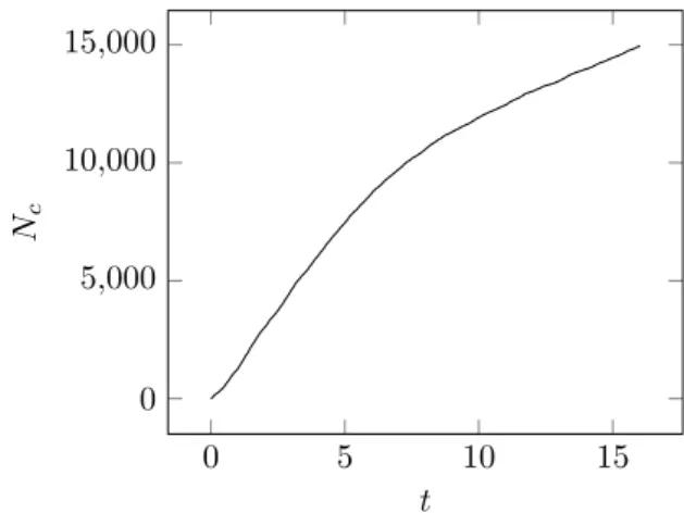
The cumulative number of particles in contact, Nc, is shown
by the Figure 3. One can observe at 10 s , that Nchas a linear
time-evolution indicating also a steady-state. From the cumula-tive number of particles in contact, the collision frequency in the whole box can be computed as
fc= 1 2
d
dt(Nc) (1)
and the inter-particle collision timescale reads τc=
Np
2fc
(2) The Table 3 shows the time-average values of the inter-particle collision frequency and timescale for each case.
Table 3: Collision frequency and collision time-scale.
CASE fc τc
A 260 col/s 0.7346 s B 1049 col/s 1.0924 s C 4315 col/s 0.04426 s D 28675 col/s 0.01998 s
Interestingly, at steady-state, for the case A, all the particles tend to migrate to centre of the flow, and at the opposite, for the
case C, they tend to migrate towards to the wall, that is high-lighted at the Figure 4.
0
5
10
15
0
5,000
10,000
15,000
t
N
cFigure 3: Cumulative number of particle in contact (Nc) for the
case A.
Figure 4: Effect of the wall slip velocity on the instantaneous dis-tribution of particles at steady-state in case A (top) and case C (bottom). The particle volume fraction is αp,bulk=5%.
Figure 4 shows instantaneous particle distribution found at steady-state for the same solid volume fraction (αp,bulk =5%) but different wall velocity. On can observed that for the low ve-locity (case A) the particles are much more located at the centre of the domain. Large-scale clusters are also found. In contrast, for Vw=3.42 m/s the particle distribution is much more uniform across the domain.
Figure 5: Effect of the particle volume fraction on the instanta-neous distribution of particles at steady-state in case A (top) and case B (bottom). The wall slip velocity is Vw=1.14 m/s.
Figure 5 shows the instantaneous particle distributions for the same wall velocity (Vw=1.14 m/s) but different particle volume fractions. As expected, increasing the particle volume fraction leads to increase the inter-particle collisions and then the parti-cles are much more uniformly distributed in the domain. 4. Results and discussion
The time-average variables, shown in this section, are com-puted at the steady-state and during a sufficiently long time in order to get converged statistics. The focus is made on the case C. −1 −0.5 0 0.5 1 −1 −0.5 0 0.5 1 2y/H Up,i / Vw
Figure 6: Mean particle velocity normalized by the wall slip velocity with respect to the wall-distance. The symbols are
: Up,x/Vw; : Up,y/Vw; : Up,z/Vw
The mean particle velocities are shown by Figure 6. Wall-normal and spanwise mean particle velocities are equal to zero. In contrast the streamwise particle velocity exhibit a linear shear in the core of the flow.
−1 −0.5 0 0.5 1 0 20 40 60 2y/H S t
Figure 7: Stokes number with respect to the wall-distance. Figure 7 shows the Stokes number profile. It is defined as St = τp∂Up,x/∂y where the particle response time is given by
τp=ρpd2p/18µf. At the centre of the domain the Stokes number
profile is about 20 and increases close to the two moving wall. As τpis given constant, the evolution of the Stokes number is
com-ing from change of the velocity shear across the channel which, in this case, is roughly constant for 2y/H between -0.3 and +0.3. As shown by Figure 8 the wall-normal distribution of the par-ticles across the domain is not uniform. The parpar-ticles are more present in the near wall region and less in the core of the domain.
−1 −0.5 0 0.5 1 0.6 0.8 1 1.2 2y/H np / np,bulk
Figure 8: Particle number density with respect to the wall-distance.
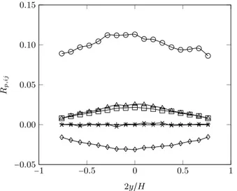
The particle kinetic stress tensor is defined by Rp,ij = ⟨u′
p,iu ′
p,j⟩pwhere u′p,iis the particle velocity fluctuation.
Fig-ure 10 shows all components of the particle kinetic stress tensor with respect to the distance with the wall. It shows that the par-ticle agitation in strongly anisotropic and is measured essentially in the streamwise direction. The spanwise and the wall-normal particle kinetic stress component are nearly the same. In addition Rp,xzand Rp,yzare found close to zero. As expected the shear
The particle kinetic agitation corresponds to the trace of the particle kinetic stress tensor. Then it is defined by q2p=1/2Rp,ii.
−1 −0.5 0 0.5 1 0.05 0.06 0.07 0.08 2y/H q 2 p
Figure 9: Particle kinetic agitation q2pwith respect to the
wall-distance. −1 −0.5 0 0.5 1 −0.05 0.00 0.05 0.10 0.15 2y/H Rp,ij
Figure 10: Particle kinetic stress tensor Rp,ijwith respect to the
wall-distance. The symbols are : Rp,xx; : Rp,yy; :
Rp,zz; : Rp,xy; : Rp,xzand : Rp,yz
The profile of qp2is shown by Figure 9. One can notice that
the agitation of the particles is higher at the centre of the domain, where particle volume fraction is lower.
In the framework of a statistical description of granular flow [7] the transport equation of each moment of the particulate phase can be derived. By assuming that Up,y, Up,zand the gradient in
x- and z-direction are negligibles , momentum equation writes ∂Up,i ∂t = − 1 np ∂ (npRp,iy) ∂y + ⟨a f i⟩p+ 1 npC (u p,i) (3) where ⟨afi⟩pis the acceleration of the particles due to fluid
inter-action.
Budget balance of Eq. (3), in the y- direction, is shown by Fig-ure 11. One can notice that a balance is established between the production term, which tends to move the particles towards the walls and and the fluid interaction term which leads the particles towards the centre.
−1 −0.5 0 0.5 1 −1 −0.5 0 0.5 1 2y/H
Figure 11: Budget analysis of the transport equation of Up,y
given by Eq. (3). The symbols are : −1/np∂ (npRp,yy) /∂y; : ⟨ay⟩p; :C (up,i) /np; : sum of all terms.
The particle kinetic tensor transport equation can also be derived. With the same assumptions, the equations for Rp,xx,
Rp,yy, Rp,zz,Rp,xyand q2pread
∂Rp,xx ∂t = − 1 np ∂ (npSp,yxx) ∂y −2Rxy ∂Up,x ∂y (4) + 2⟨afxu′p,x⟩p+ 1 np C (u′ p,xu ′ p,x) ∂Rp,yy ∂t = − 1 np ∂ (npSp,yyy) ∂y (5) + 2⟨afyu′p,y⟩p+ 1 np C (u′ p,yu ′ p,y) ∂Rp,zz ∂t = − 1 np ∂ (npSp,yzz) ∂y (6) + 2⟨afzu′p,z⟩p+ 1 npC (u ′ p,zu ′ p,z) ∂Rp,xy ∂t = − 1 np ∂ (npSp,xyy) ∂y −Rp,yy ∂Up,x ∂y (7)
+ ⟨afxu′p,y⟩ + ⟨afyu′p,x⟩p+ 1 npC (u ′ p,xu ′ p,y) ∂q2 p ∂t = − 1 2np ∂ (npSp,yii) ∂y −Rxy ∂Up,x ∂y (8) + ⟨afiu′p,i⟩ + 1 npC (u ′ p,iu ′ p,i)
In Eqs. (4)-(8), Sp,ijk= ⟨u ′ p,iu
′ p,ju
′
p,k⟩is the third order cor-relation of the particle fluctuating velocity. Figure 12 - 15 shows each contribution of Eq. (4) - Eq. (7). One can observe that in x-direction the particle kinetic stress is produced by the mean shear. As expected the friction of the particles with the fluid leads to the destruction of the particle kinetic stress component Rp,xx, Rp,yy,
Rp,zz and Rp,xy. In the x- and z- direction the inter-particle
interactions is negative meaning that the collisions decrease the particle kinetic stress component. In contrast in y-direction the inter-particle interaction term is positive meaning that the colli-sions increase Rp,yyand Rp,zz. This effect is due to the nature
of the collisions that is an isotropization effect. In the present case, the particle agitation in x-direction is redistributed towards y- and z-direction by the inter-particle collision [10]. Such kind of behavior has also been found at [11, 12].
A diffusive term is also found near the centre of the domain for the budgets of Rp,xx, Rp,yy and Rp,xy, this effect leads to the
transport of agitation away of the centre.
−1 −0.5 0 0.5 1 −4 −2 0 2 4 2y/H
Figure 12: Budget analysis of the transport equa-tion of Rp,xx given by Eq. (4). The symbols are
: −1/np∂ (npSp,yxx) /∂y; : −2Rxy∂Up,x/∂y; : 2⟨afxu
′
p,x⟩p; :C (u′p,xu ′
p,x) /np; : sum of all the
terms.
The terms of the evolution of the particle agitation equation given by Eq. (8) are depicted by Figure 16. One can notice that the global effect is that the random kinetic energy is produced by the mean particle shear velocity, and it is dissipated by the colli-sions and the interaction with the fluid.
−1 −0.5 0 0.5 1 −0.4 −0.2 0 0.2 0.4 2y/H
Figure 13: Budget analysis of the transport equa-tion of Rp,yy given by Eq. (5). The symbols are
: −1/np∂ (npSp,yyy) /∂y; : 2⟨afyu ′ p,y⟩p;
:C (u′ p,yu
′
p,y) /np; : sum of all terms.
−1 −0.5 0 0.5 1 −0.4 −0.2 0 0.2 0.4 2y/H
Figure 14: Budget analysis of the transport equa-tion of Rp,zz given by Eq. (6). The symbols are
: −1/np∂ (npSp,yzz) /∂y; : 2⟨afzu′p,z⟩p;
:C (u′ p,zu
′
p,z) /np; : sum of all terms.
−1 −0.5 0 0.5 1 −1 −0.5 0 0.5 1 2y/H
Figure 15: Budget analysis of the transport equa-tion of Rp,xy given by Eq. (7). The symbols are
: −1/np∂ (npSp,xyy) /∂y; : −Rp,yy∂Up,x/∂y;
: ⟨afxu ′ p,y⟩ + ⟨a f yu ′ p,x⟩p; : C (u′p,xu ′ p,y) /np; :
−1 −0.5 0 0.5 1 −2 −1 0 1 2 2y/H
Figure 16: Budget analysis of the transport equa-tion of q2p given by Eq. (8). The symbols are
: −1/ (2np)∂ (npSp,ykk) /∂y; : −Rxy∂Up,x/∂y;
: ⟨afku′ p,k⟩p; :C (u′p,ku ′ p,k) / (2np); : sum of all terms. 5. Conclusion
3D dense fluid-particle Couette flow were studied using di-rect numerical simulation. Fundamental parameters of the flow have been extracted from the steady-state such as, particle kinetic stress tensor, third order correlation, collision time-scale, etc. The production, diffusion, collisional and fluid interaction terms were analyzed highlighting fundamental physics of the flow, such as the isotropization effect with the collisions.
6. Acknowledgments
The authors acknowledge the support from the Brazilian funding agency CAPES (Science-Without-Borders - scholarship: 13172-13-1). This work was granted access to the HPC resources of CALMIP supercomputing center under the allocation 2015-[p0111] and 2016-[p1529].
References
[1] S. Chapman, T. G. Cowling, The mathematical theory of non-uniform gases: an account of the kinetic theory of vis-cosity, thermal conduction and diffusion in gases. Cam-bridge university press., 1970.
[2] A.T. Cate, J.J. Derksen, L.M. Portela, H.E.A. Van Den Akker, Fully resolved simulations of colliding monodis-perse spheres in forced isotropic turbulence. Journal of Fluid Mechanics, 519, 2004.
[3] J.C. Brändle de Motta, W.-P. Breugem, B. Gazanion, J.-L. Estivalèzes, S. Vincent, E. Climent, Numerical modelling of finite-size particle collision in a viscous fluid. Phys. Fluids, 25, 083302, 2013.
[4] J.C. Brändle de Motta, Simulation des ecoulements turbu-lents avec des particules de taille finie en regime dense. PhD Thesis, Institut Supérieur de l’Aeronautique et de l’Espace (ISAE), 2013.
[5] T.N. Randrianarivelo, Etude numérique des interactions hydrodynamiques fluides/solides: application aux lits flu-idisés. PhD thesis, Bordeaux 1, 2005.
[6] A.J. Sarthou, Méthodes de domaines fictifs d’ordre élevé pour les équations elliptiques et de Navier-Stokes: applica-tion au couplage fluide-structure. PhD thesis, Bordeaux 1, 2009.
[7] O. Simonin, Continuum modelling of dispersed two-phase flows. Lecture Series 1996-02, von Karman Institute for Fluid Dynamics, K1-K47, 1996.
[8] M. Uhlmann, An immersed boundary method with direct forcing for the simulation of particulate flows. Journal of Computational Physics, 448 - 476, 209, 2005.
[9] S. Vincent, J.C. Brändle de Motta, A. Sarthou, J.-L. Esti-valèzes, O. Simonin, E. Climent, A Lagrangian VOF tenso-rial penalty method for the DNS of resolved particle-laden flows. Journal of Computational Physics, vol. 256, pp. 582-614, 2014
[10] N. Caraman, J. Borée, and O. Simonin. Effect of collisions on the dispersed phase fluctuation in a dilute tube flow: Experimental and theoretical analysis. Physics of Fluids, 15.12: 3602-3612, 2003
[11] J. F. Parmentier, O. Simonin. Transition models from the quenched to ignited states for flows of inertial particles sus-pended in a simple sheared viscous fluid. Journal of Fluid Mechanics, 711, 147-160, 2012.
[12] A. Boëlle, G. Balzer, O. Simonin. Second-order prediction of the particle-phase stress tensor of inelastic spheres in simple shear dense suspensions. ASME-PUBLICATIONS-FED, 228, 9-18, 1995