Multi-scale Analysis of the Fatigue of Shape Memory Alloys

HAL Id: tel-01422026

https://pastel.archives-ouvertes.fr/tel-01422026

HAL is a multi-disciplinary open access archive for the deposit and dissemination of sci-entific research documents, whether they are pub-lished or not. The documents may come from teaching and research institutions in France or abroad, or from public or private research centers.

L’archive ouverte pluridisciplinaire HAL, est destinée au dépôt et à la diffusion de documents scientifiques de niveau recherche, publiés ou non, émanant des établissements d’enseignement et de recherche français ou étrangers, des laboratoires publics ou privés.

Multi-scale Analysis of the Fatigue of Shape Memory

Alloys

Lin Zheng

To cite this version:

Lin Zheng. Multi-scale Analysis of the Fatigue of Shape Memory Alloys. Mechanics of the solides [physics.class-ph]. Université Paris-Saclay, 2016. English. �NNT : 2016SACLY011�. �tel-01422026�

NNT : 2016SACLY011

T

HESE DE

D

OCTORAT

DE

L

’U

NIVERSITE

P

ARIS

-S

ACLAY

PREPAREE A

L

’E

COLE

N

ATIONALE

S

UPERIEURE DE

T

ECHNIQUES

A

VANCEES

ÉCOLE DOCTORALE N°579

Sciences Mécaniques et Energétiques, Matériaux et Géosciences

Spécialité de doctorat : Mécanique des Solides

Par

Mme Lin ZHENG

Multi-scale Analysis of the Fatigue of Shape Memory Alloys

Thèse présentée et soutenue à Palaiseau, le 28 septembre 2016: Composition du Jury :

M. E. Charkaluk, Directeur de Recherche, Université Lille1 Sciences et Technologies, Président M. T. Ben Zineb, Professeur des Universités, Université de Lorraine (LEMTA – ESSTIN), Rapporteur Mme S. Arbab Chirani, Professeure des Universités, Ecole Nationale d'Ingénieurs de Brest, Rapporteur M. J.-J. Marigo, Professeur, Ecole Polytechnique, Examinateur

M. Y.J. He, Maître de Conférences (HDR), ENSTA-ParisTech, Co-directeur de thèse M. Z. Moumni, Professeur, ENSTA-ParisTech, Directeur de thèse

Université Paris-Saclay

Espace Technologique / Immeuble Discovery

T

HESE DE

D

OCTORAT

DE

L

’U

P

-S

L

’E

N

S

T

A

ÉCOLE DOCTORALE N°579

Sciences Mécaniques et Energétiques, Matériaux et Géosciences

Spécialité de doctorat : Mécanique des Solides

Par

Mme Lin ZHENG

Multi-scale Analysis of the Fatigue of Shape Memory Alloys

Thèse présentée et soutenue à Palaiseau, le 28 septembre 2016: Composition du Jury :

M. E. Charkaluk, Directeur de Recherche, Université Lille1 Sciences et Technologies, Président M. T. Ben Zineb, Professeur des Universités, Université de Lorraine (LEMTA – ESSTIN), Rapporteur Mme S. Arbab Chirani, Professeure des Universités, Ecole Nationale d'Ingénieurs de Brest, Rapporteur M. J.-J. Marigo, Professeur, Ecole Polytechnique, Examinateur

M. Y.J. He, Maître de Conférences (HDR), ENSTA-ParisTech, Co-directeur de thèse M. Z. Moumni, Professeur, ENSTA-ParisTech, Directeur de thèse

ii

Dedicated to my beloved grandmother and mother.



2016

iv

Publications

L. Zheng, Y.J. He, Z. Moumni, 2015. Frequency-dependent temperature and strain evolutions of NiTi wire during cyclic stress-controlled martensitic transformation, Proceeding of PCM-CMM-2015, Gdansk, Poland.

L. Zheng, Y.J. He, Z. Moumni, 2016. Effects of Lüders-like bands on NiTi fatigue behaviors, International Journal of Solids and Structures 83 (2016) 28-44. doi:10.1016/j.ijsolstr.2015.12.021.

L. Zheng, Y.J. He, Z. Moumni, 2016. Lüders-like band front motion and fatigue life of pseudoelastic polycrystalline NiTi shape memory alloy, Scripta Materialia 123 (2016) 46-50. doi:10.1016/j.scriptamat.2016.05.042.

L. Zheng, Y.J. He, Z. Moumni, 2016. Investigation on fatigue behaviors of NiTi polycrystalline strips under stress-controlled tension via in-situ macro-band observation, under review.

Acknowledgement

To write this acknowledgement is kind of to recall all the memories I had in this lab for more than three years. There were tough moments but also happy ones and I am grateful for arriving at the final line.

My two supervisors, Ziad Moumni and Yongjun He, this work would not have been possible without you. Ziad, thank you for creating the best working conditions (experimental materials, personal office, etc.) and meeting my other wants as possible as you can. Yongjun, you are the person who has watched me from the very beginning to the end, shared your own experiences (good and bad) in Hong Kong with no reservations, pointed out my faults of doing researches and then encouraged me by saying the merits in me and even listened to my complaints and tolerated my bad moods. So, thank you so much for devoting your precious time to me.

The two department directors, previously Antoine Chaigne and Habibou Maitournam since 2014, thank you for your efforts to advance my work.

I would also like to acknowledge all my committee members, Professors Eric Charkaluk, Jean-Jacques Marigo, Shabnam Arbab Chirani, and Tarak Ben Zineb, for your time and efforts devoted to evaluate my work.

It is a pleasure to thank all the faculty and staff –– particularly, Anne-Lise Gloanec, Boumediene Nedjar, Kim Pham, thank you for your advice and concern; Alain Van Herpen and Lahcène Cherfa, thanks so much for your help with my experiments; Nicolas Baudet and Thierry Pichon, thank you for your support on the hardware and software. And all the fellow PhD students and postdocs, Agathe Forré, Ammar Ould Amer, Hao Yin, Jun Wang, Nicolas Thurieau, Oana-Zenaida Pascan, Qi Peng, Qianqiang Chen, Quantin Pierron, Selçuk Hazar, Shaobin Zhang, Xiaojun Gu, Xue Chen, Yahui Zhang, and Yinjun Jiang who is a visiting researcher from China, I have been fortunate to have shared the common moments in the lab with all of you. Also thank you to the two master students, Asma El Elmi and Ren Wei, who were with me on some experiments.

Last, but certainly not least, thank you to Shanshan Geng, who in the past four years has been with me through thick and thin and always believed in me. I am lucky and happy to be your friend.

vi

Table of Contents

Table of Figures ··· vii

Chapter 1 Introduction ··· 1

Chapter 2 Significant Effects of Lüders-like Bands on NiTi Fatigue Behaviors 10 2.1 Introduction ··· 10

2.2 Material and experimental details ··· 11

2.3 Experimental observation ··· 12

2.4 Discussion ··· 25

Chapter 3 Relation between Lüders-like Band-front Motion and Fatigue ··· 31

3.1 Introduction ··· 31

3.2 Results and discussion ··· 33

3.3 Summary ··· 43

Chapter 4 Band-Pattern Evolutions and Material Fatigue Criterion ··· 45

4.1 Introduction ··· 45

4.2 Experimental results ··· 46

4.3 Discussion ··· 78

4.4 Conclusions ··· 83

Chapter 5 Conclusions and Prospects ··· 85

Appendix: Experimental results of Specimens B, C, E~H of Chapter 2 ··· 90

References ··· 102

Table of Figures

Fig. 1.1 Schematics of (a) shape memory effect and (b) pseudoelasticity. Fig. 1.2 Multi-scale structures in NiTi polycrystals.

Fig. 1.3 Specifications of the NiTi dog-bone shaped specimen Fig. 2.1 Cyclic waveform under stress control

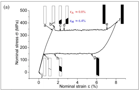
Fig. 2.2 (a) Nominal stress-strain response curve with schematic patterns demonstrating the Lüders-like band evolution in a NiTi strip (Specimen A) in a strain-controlled tensile cycle (low strain rate 𝜀𝜀̇ = 8×10-5 _s-1_{, approximated as an isothermal case). The black and white} regions of the schematic patterns respectively represent the Martensite (M) and Austenite (A) domains in the gauge section of the dog-bone specimen. (b) Optical observation on the Lüders-like bands. Values of the applied nominal strain 𝜀𝜀 are accompanied by the symbol ↗ (↘) denoting the loading (unloading) process.

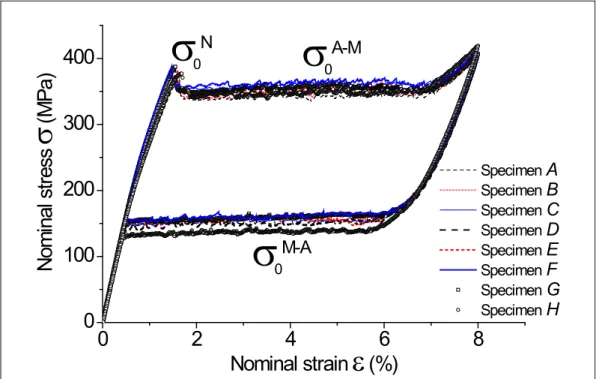
Fig. 2.3 All the 8 tested specimens have similar stress-strain curves of the isothermal strain-controlled test with strain rate 𝜀𝜀̇ = 8×10-5 _s-1_.

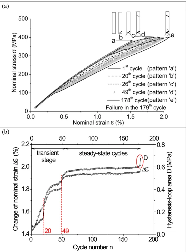
Fig. 2.4 The stress-controlled tensile fatigue test on Specimen A with the maximum stress

𝜎𝜎𝑚𝑚𝑚𝑚𝑚𝑚 = 400 MPa and the frequency 𝑓𝑓 = 1 Hz (Lüders-like band appeared before the

“steady-state” cycles): (a) stress-strain curve evolution and schematic patterns, (b) evolutions of the cycle features: strain change ∆𝜀𝜀 and mechanical energy-dissipation density 𝐷𝐷 in one cycle, and (c) optical observation on the Lüders-like bands (the leftmost image shows the band nucleation in the isothermal test for reference).

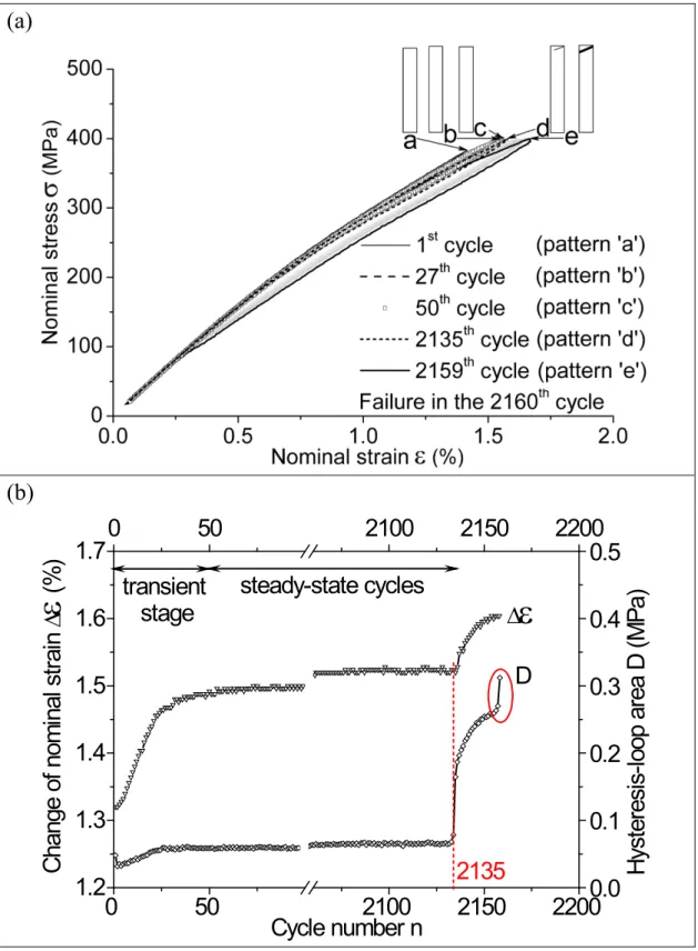
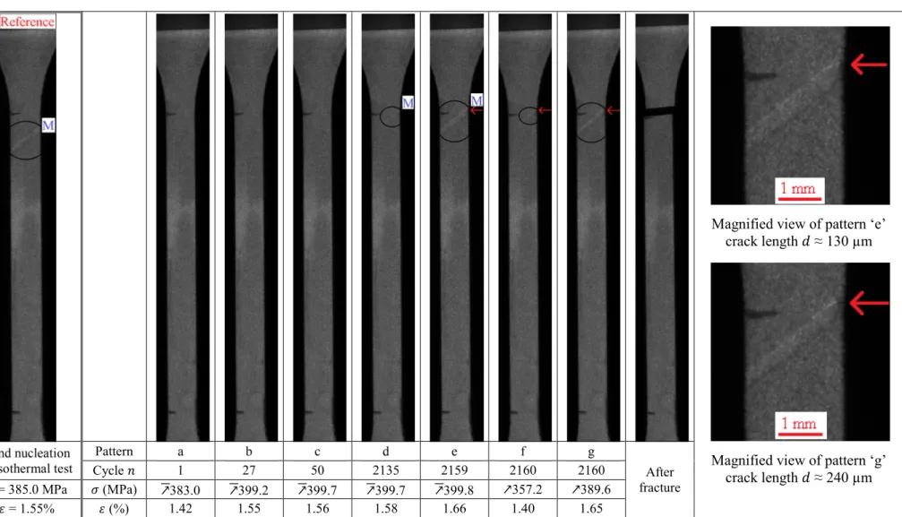
Fig. 2.5 The stress-controlled tensile fatigue test on Specimen D with 𝜎𝜎𝑚𝑚𝑚𝑚𝑚𝑚 = 400 MPa and 𝑓𝑓

= 1 Hz (Lüders-like band appeared after the “steady-state” cycles): (a) stress-strain curve evolution and schematic patterns, (b) evolutions of the cycle features ∆𝜀𝜀 and 𝐷𝐷, and (c) optical observation on the Lüders-like bands (the leftmost image shows the band nucleation in the isothermal test for reference).

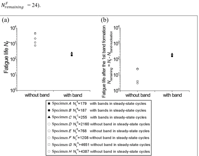
Fig. 2.6 Effects of the band formation (i.e., with/without the band nucleation/annihilation in “steady-state” cycles) on: (a) the fatigue life 𝑁𝑁𝑓𝑓, (b) the remaining fatigue life after the 1st band

formation 𝑁𝑁𝑟𝑟𝑟𝑟𝑚𝑚𝑚𝑚𝑟𝑟𝑟𝑟𝑟𝑟𝑟𝑟𝑟𝑟 .

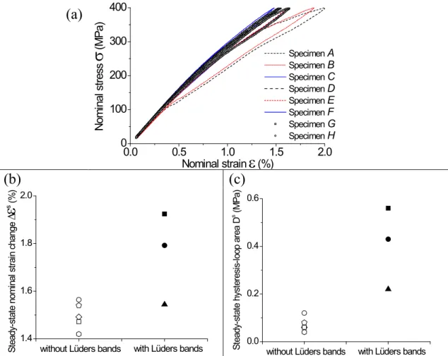
Fig. 2.7 Effects of the band formation on the mechanical responses of the “steady stage”: (a) stress-strain curve of the 1st _{“steady-state” cycle, (b) nominal strain change ∆𝜀𝜀}𝑠𝑠_{, and (c)}

mechanical energy-dissipation density 𝐷𝐷𝑠𝑠_{. (Legend of (b) and (c) is the same as in Fig. 2.6)}

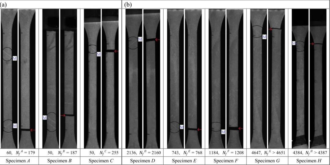
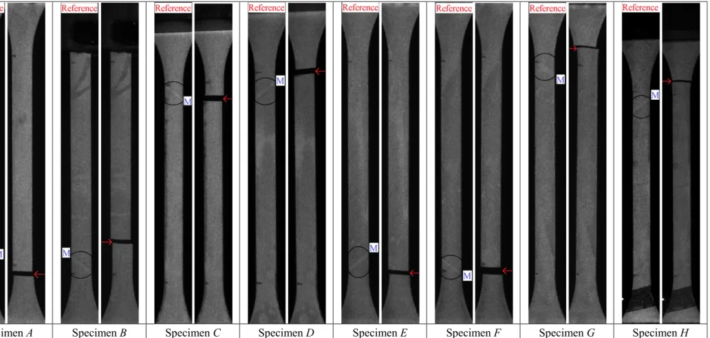
Fig. 2.8 (a) Comparisons between the band locations in the 1st _{“steady-state” cycles and the} fatigue failure positions of Specimens A~C. (b) Comparisons between the locations of the 1st band nucleation and the fatigue failure positions of Specimens D~H.

Fig. 2.9 Comparisons between the location of the band formation in the reference isothermal test (left) and the fatigue failure position (right).

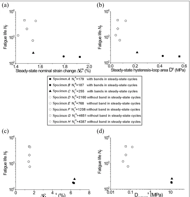
Fig. 2.10 Correlations between the fatigue life 𝑁𝑁𝑓𝑓 and the structure responses in the “steady

stage”: (a) change of structural nominal strain ∆𝜀𝜀𝑠𝑠_{, and (b) structural mechanical}

energy-dissipation density 𝐷𝐷𝑠𝑠_{. Correlations between the fatigue life 𝑁𝑁}

𝑓𝑓 and the material responses in

viii

the “steady stage”: (c) material’s strain change ∆𝜀𝜀𝑚𝑚𝑚𝑚𝑚𝑚𝑟𝑟𝑟𝑟𝑟𝑟𝑚𝑚𝑚𝑚𝑠𝑠 , and (d) material’s mechanical

energy-dissipation density 𝐷𝐷_{𝑚𝑚𝑚𝑚𝑚𝑚𝑟𝑟𝑟𝑟𝑟𝑟𝑚𝑚𝑚𝑚}𝑠𝑠 _.

Fig. 3.1 Cyclic waveform under strain control

Fig. 3.2 DIC measurement of the local strains for two typical cases (nominal strain amplitude

𝜀𝜀𝑚𝑚𝑚𝑚𝑎𝑎𝑚𝑚 = 1.0% and 0.5%): (a) fully-developed “active zone” and (b) partially-developed “active

zone” whose size is comparable to the band-front thickness.

Fig. 3.3 (a) Nominal stress-strain curves of fatigue cycles (solid lines: the black, blue, red lines respectively represent the 1st_{, the 100}th_{, and the final cycle before failure) of the specimens} under a fixed nominal mean strain (𝜀𝜀𝑚𝑚𝑟𝑟𝑚𝑚𝑟𝑟 = 3.5%) with different nominal strain amplitudes

(𝜀𝜀𝑚𝑚𝑚𝑚𝑎𝑎𝑚𝑚 = 1.5%~0.25%) in comparison with their isothermal curves (dashed lines); (b) The

corresponding Lüders-like band evolution (with “active zones” (shaded zones) in Cases I~V and without “active zones” in Case VI) and the final fractured specimens, where the red arrows indicate the fatigue-failure crack nucleation positions.

Fig. 3.4 Dependences of the fatigue life 𝑁𝑁𝑓𝑓 on (a) the size of “active zones” l and (b) the local

strain amplitude 𝜀𝜀𝑚𝑚𝑚𝑚𝑎𝑎𝑚𝑚𝑚𝑚𝑙𝑙𝑙𝑙𝑚𝑚𝑚𝑚 of the fatigue-failure material points.

Fig. 3.5 (a) The deformation domains and the final fractured specimens in the fatigue tests with a fixed nominal strain amplitude 𝜀𝜀𝑚𝑚𝑚𝑚𝑎𝑎𝑚𝑚 = 0.25% (no “active zones”) and different

nominal mean strains 𝜀𝜀𝑚𝑚𝑟𝑟𝑚𝑚𝑟𝑟 (note: the specimen didn’t fail after 32922 cycles in Case I).

Fig. 3.6 (a) The dependence of the fatigue life 𝑁𝑁𝑓𝑓 on 𝜀𝜀𝑚𝑚𝑟𝑟𝑚𝑚𝑟𝑟; (b) The dependence of 𝑁𝑁𝑓𝑓 on the

local mean strain 𝜀𝜀𝑚𝑚𝑟𝑟𝑚𝑚𝑟𝑟𝑚𝑚𝑙𝑙𝑙𝑙𝑚𝑚𝑚𝑚 (solid/open symbols represent the tests with/without fracture failure).

Fig. 3.7 (a) Global observation by optical camera on a specimen with small cyclic “active zones” (shaded zones) under the nominal strain amplitude of 0.5% and (b) Local observation by microscope on the evolution of a macro crack at the left end of the upper band front in (a). Fig. 4.1 All the tested specimens have similar stress-strain curves in the isothermal strain-controlled tensile tests with global strain rate of 8×10-5 _s-1_{. 𝜎𝜎}

0A→M ( 𝜎𝜎0M→A) denotes the

transformation stress during the Austenite (A)→ Martensite (M) (M→A) phase transformation and 𝜎𝜎0N denotes the band-nucleation stress at room temperature 𝑇𝑇0 ≈ 21°C.

Fig. 4.2 The stress-controlled cyclic tensile test on Specimen 𝑇𝑇 with the maximum stress 𝜎𝜎𝑚𝑚𝑚𝑚𝑚𝑚

= 500 MPa and the loading frequency 𝑓𝑓 = 0.01 Hz for 50 cycles: (a) the evolution of the stress-strain 𝜎𝜎 − 𝜀𝜀 curve, (b) evolutions of cycle-minimum nominal strain 𝜀𝜀𝑚𝑚𝑟𝑟𝑟𝑟 ,

cycle-maximum nominal strain 𝜀𝜀𝑚𝑚𝑚𝑚𝑚𝑚 , and nominal strain change ∆𝜀𝜀 = 𝜀𝜀𝑚𝑚𝑚𝑚𝑚𝑚 − 𝜀𝜀𝑚𝑚𝑟𝑟𝑟𝑟 , (c) the

evolution of the mechanical energy-dissipation density 𝐷𝐷. (d) The optical observation on the Lüders-like band patterns of Specimen 𝑇𝑇. The values of the applied stress are accompanied by the symbol ↗ (↘) denoting the loading (unloading) process, zones highlighted by the black circles are the newly nucleated M bands during loading (patterns ‘a’~’e’ and ‘i’~‘j’), the residual A bands at the end of loading (pattern ‘f’), or the residual M bands at the end of unloading (patterns ‘h’ and ‘l’). (e) The DIC full-field strain maps corresponding to the optical patterns in (d). (f) The local strain profiles derived from the DIC strain maps in (e) show the strain distribution along the centerline of the specimen’s gauge section.

Fig. 4.3 The stress-controlled tensile fatigue test on Specimen 𝐴𝐴₅₀₀0.01 _{with 𝜎𝜎}

𝑚𝑚𝑚𝑚𝑚𝑚 = 500 MPa and

𝑓𝑓 = 0.01 Hz: (a) the evolution of 𝜎𝜎 − 𝜀𝜀 curve, (b) evolutions of 𝜀𝜀𝑚𝑚𝑟𝑟𝑟𝑟, 𝜀𝜀𝑚𝑚𝑚𝑚𝑚𝑚, and ∆𝜀𝜀 = 𝜀𝜀𝑚𝑚𝑚𝑚𝑚𝑚 −

𝜀𝜀𝑚𝑚𝑟𝑟𝑟𝑟, (c) the evolution of 𝐷𝐷, and (d) the optical observation on the Lüders-like band patterns.

Fig. 4.4 (a) Illustration of the shaded “active zones” with A↔M phase transformation and the unshaded “non-active zones” with “elastic” deformation of residual M bands in the 1st _fatigue cycle of Specimen 𝐴𝐴5000.01 compared with an image of the specimen after fracture failure; (b)

The nominal stress-strain curve, 5 optical and DIC patterns, the associated strain profiles along the centerline of specimen’s gauge section and the calculated local strain amplitude 𝜀𝜀𝑚𝑚𝑚𝑚𝑎𝑎𝑚𝑚𝑚𝑚𝑙𝑙𝑙𝑙𝑚𝑚𝑚𝑚 in

the 1st _cycle.

Fig. 4.5 (a) Illustration of the shaded “active zones” with A↔M phase transformation and the unshaded “non-active zones” with “elastic” deformation of residual M bands in the 50th _fatigue cycle of Specimen 𝐴𝐴5000.01 compared with an image of the specimen after fracture failure; (b)

The nominal stress-strain curve, 5 optical and DIC patterns, the associated strain profiles along the centerline of specimen’s gauge section and the calculated local strain amplitude 𝜀𝜀𝑚𝑚𝑚𝑚𝑎𝑎𝑚𝑚𝑚𝑚𝑙𝑙𝑙𝑙𝑚𝑚𝑚𝑚 in

the 50th _cycle.

Fig. 4.6 The stress-controlled tensile fatigue test on Specimen 𝐴𝐴5000.1 with 𝜎𝜎𝑚𝑚𝑚𝑚𝑚𝑚 = 500 MPa and

𝑓𝑓 = 0.1 Hz: (a) the evolution of 𝜎𝜎 − 𝜀𝜀 curve, (b) evolutions of 𝜀𝜀𝑚𝑚𝑟𝑟𝑟𝑟, 𝜀𝜀𝑚𝑚𝑚𝑚𝑚𝑚, and ∆𝜀𝜀 = 𝜀𝜀𝑚𝑚𝑚𝑚𝑚𝑚 −

𝜀𝜀𝑚𝑚𝑟𝑟𝑟𝑟, (c) the evolution of 𝐷𝐷, and (d) the optical observation on the Lüders-like band patterns.

Fig. 4.7 (a) Comparison of the “active zones” (shaded zones) and the “non-active zones” (residual A or residual M bands) in the 1st _{cycle, the 7}th _{cycle, and the 50}th _{fatigue cycle of} Specimen 𝐴𝐴₅₀₀0.1 _{; The nominal 𝜎𝜎 − 𝜀𝜀 curves, the typical strain profiles and the calculated local}

strain amplitudes 𝜀𝜀_{𝑚𝑚𝑚𝑚𝑎𝑎𝑚𝑚}𝑚𝑚𝑙𝑙𝑙𝑙𝑚𝑚𝑚𝑚 _{in the 1}st _{cycle (b), in the 7}th _{cycle (c) and in the 50}th _{cycle (d).}

Fig. 4.8 The stress-controlled tensile fatigue test on Specimen 𝐴𝐴1500 with 𝜎𝜎𝑚𝑚𝑚𝑚𝑚𝑚 = 500 MPa and

𝑓𝑓 = 1 Hz: (a) the evolution of 𝜎𝜎 − 𝜀𝜀 curve, (b) evolutions of 𝜀𝜀𝑚𝑚𝑟𝑟𝑟𝑟, 𝜀𝜀𝑚𝑚𝑚𝑚𝑚𝑚, and ∆𝜀𝜀 = 𝜀𝜀𝑚𝑚𝑚𝑚𝑚𝑚 −

ε_min, (c) the evolution of 𝐷𝐷, and (d) the optical observation on the Lüders-like band patterns. Fig. 4.9 (a) Comparison of the “active zones” (shaded zones) and the “non-active zones” (residual A bands) in the 10th _{cycle and the 50}th _{fatigue cycle of Specimen 𝐴𝐴}

500

1 _{; The nominal}

𝜎𝜎 − 𝜀𝜀 curves, the typical strain profiles and the calculated local strain amplitudes 𝜀𝜀𝑚𝑚𝑚𝑚𝑎𝑎𝑚𝑚𝑚𝑚𝑙𝑙𝑙𝑙𝑚𝑚𝑚𝑚 in the

10th _{cycle (b) and in the 50}th _{cycle (c).}

Fig. 4.10 The stress-controlled tensile fatigue test on Specimen 𝐴𝐴0.01400 with 𝜎𝜎𝑚𝑚𝑚𝑚𝑚𝑚 = 400 MPa

and 𝑓𝑓 = 0.01 Hz; (a) the evolution of 𝜎𝜎 − 𝜀𝜀 curve, (b) evolutions of 𝜀𝜀𝑚𝑚𝑟𝑟𝑟𝑟, 𝜀𝜀𝑚𝑚𝑚𝑚𝑚𝑚, and ∆𝜀𝜀 =

𝜀𝜀𝑚𝑚𝑚𝑚𝑚𝑚 − 𝜀𝜀𝑚𝑚𝑟𝑟𝑟𝑟, (c) the evolution of 𝐷𝐷, and (d) the DIC strain maps demonstrating the

Lüders-like band patterns.

Fig. 4.11 The stress-controlled tensile fatigue test on Specimen 𝐴𝐴4000.1 with 𝜎𝜎𝑚𝑚𝑚𝑚𝑚𝑚 = 400 MPa

and 𝑓𝑓 = 0.1 Hz: (a) the evolution of 𝜎𝜎 − 𝜀𝜀 curve, (b) evolutions of 𝜀𝜀𝑚𝑚𝑟𝑟𝑟𝑟, 𝜀𝜀𝑚𝑚𝑚𝑚𝑚𝑚, and ∆𝜀𝜀 =

𝜀𝜀𝑚𝑚𝑚𝑚𝑚𝑚 − 𝜀𝜀𝑚𝑚𝑟𝑟𝑟𝑟, (c) the evolution of 𝐷𝐷, and (d) the DIC strain maps demonstrating the

Lüders-like band patterns.

Fig. 4.12 Significant effects of the Lüders-like band formation in the “steady-state” cycles on the specimen’s mechanical responses and the associated fatigue life: (a) Specimen 𝐴𝐴4001 with

Lüders-like bands in the “steady-state” cycles and (b) Specimen 𝐷𝐷4001 without Lüders-like

bands in the “steady-state” cycles.

Fig. 4.13 Comparison of the nominal 𝜎𝜎 − 𝜀𝜀 curves (left), the strain profiles and the calculated local strain amplitude 𝜀𝜀_{𝑚𝑚𝑚𝑚𝑎𝑎𝑚𝑚}𝑚𝑚𝑙𝑙𝑙𝑙𝑚𝑚𝑚𝑚 _{(right) in the 50}th _{cycles of (a) Specimen 𝐴𝐴}

400

0.01_{, (b) Specimen}

𝐴𝐴4000.1 , and (c) Specimen 𝐴𝐴4001 .

x

Fig. 4.14 Evolutions of 𝜎𝜎 − 𝜀𝜀 curve of the stress-controlled tensile fatigue tests on (a) Specimen 𝐴𝐴3000.1 with 𝜎𝜎𝑚𝑚𝑚𝑚𝑚𝑚 = 300 MPa and 𝑓𝑓 = 0.1 Hz and (b) Specimen 𝐴𝐴1300 with 𝜎𝜎𝑚𝑚𝑚𝑚𝑚𝑚 = 300

MPa and 𝑓𝑓 = 1 Hz.

Fig. 4.15 (a) Typical Lüders-like band patterns under different loading conditions (shaded “active zones” with cyclic A↔M phase transformation and the unshaded “non-active zones” with cyclic “elastic” deformation of residual Martensite or residual Austenite) demonstrate the effects of the applied stress and frequency; the fatigue failure always occurred in one of the “active zones” indicated by the arrows; (b) The dependence of the fatigue life 𝑁𝑁𝑓𝑓 on the local

strain amplitude 𝜀𝜀_{𝑚𝑚𝑚𝑚𝑎𝑎𝑚𝑚}𝑚𝑚𝑙𝑙𝑙𝑙𝑚𝑚𝑚𝑚 _{in the “steady stage”; (c) The dependence of 𝑁𝑁}

𝑓𝑓 on the applied stress

and frequency, where 𝑁𝑁𝑓𝑓 basically decreases with increasing the stress level. (The dashed lines

just guide the eyes.)

Fig. 4.16 The dependences of the fatigue life 𝑁𝑁𝑓𝑓 on (a) the local residual strain 𝜀𝜀_{𝑚𝑚𝑙𝑙𝑙𝑙𝑚𝑚𝑚𝑚 −𝑟𝑟𝑟𝑟𝑠𝑠}𝑁𝑁𝑓𝑓 and

(b) the average accumulation rate of the local residual strain 𝜀𝜀_{𝑚𝑚𝑙𝑙𝑙𝑙𝑚𝑚𝑚𝑚 −𝑟𝑟𝑟𝑟𝑠𝑠}𝑁𝑁𝑓𝑓 _{= 𝜀𝜀}

𝑚𝑚𝑙𝑙𝑙𝑙𝑚𝑚𝑚𝑚 −𝑟𝑟𝑟𝑟𝑠𝑠𝑁𝑁𝑓𝑓 /𝑁𝑁𝑓𝑓.

Fig. A1 The stress-controlled tensile fatigue test on Specimen B with 𝜎𝜎𝑚𝑚𝑚𝑚𝑚𝑚 = 400 MPa and 𝑓𝑓 =

1 Hz (Lüders-like band appeared before the “steady-state” cycles): (a) stress-strain curve evolution and schematic patterns, (b) evolutions of the cycle features ∆𝜀𝜀 and 𝐷𝐷, and (c) optical observation on the Lüders-like bands.

Fig. A2 The stress-controlled tensile fatigue test on Specimen C with 𝜎𝜎𝑚𝑚𝑚𝑚𝑚𝑚 = 400 MPa and 𝑓𝑓

= 1 Hz (Lüders-like band appeared before the “steady-state” cycles): (a) stress-strain curve evolution and schematic patterns, (b) evolutions of the cycle features ∆𝜀𝜀 and 𝐷𝐷, and (c) optical observation on the Lüders-like bands.

Fig. A3 The stress-controlled tensile fatigue test on Specimen E with 𝜎𝜎𝑚𝑚𝑚𝑚𝑚𝑚 = 400 MPa and 𝑓𝑓 =

1 Hz (Lüders-like band appeared after the “steady-state” cycles): (a) stress-strain curve evolution and schematic patterns, (b) evolutions of the cycle features ∆𝜀𝜀 and 𝐷𝐷, and (c) optical observation on the Lüders-like bands.

Fig. A4 The stress-controlled tensile fatigue test on Specimen F with 𝜎𝜎𝑚𝑚𝑚𝑚𝑚𝑚 = 400 MPa and 𝑓𝑓 =

1 Hz (Lüders-like band appeared after the “steady-state” cycles): (a) stress-strain curve evolution and schematic patterns, (b) evolutions of the cycle features ∆𝜀𝜀 and 𝐷𝐷, and (c) optical observation on the Lüders-like bands.

Fig. A5 The stress-controlled tensile fatigue test on Specimen G with 𝜎𝜎𝑚𝑚𝑚𝑚𝑚𝑚 = 400 MPa and 𝑓𝑓

= 1 Hz (Lüders-like band appeared after the “steady-state” cycles): (a) stress-strain curve evolution and schematic patterns, (b) evolutions of the cycle features ∆𝜀𝜀 and 𝐷𝐷, and (c) optical observation on the Lüders-like bands.

Fig. A6 The stress-controlled tensile fatigue test on Specimen H with 𝜎𝜎𝑚𝑚𝑚𝑚𝑚𝑚 = 400 MPa and 𝑓𝑓

= 1 Hz (Lüders-like band appeared after the “steady-state” cycles): (a) stress-strain curve evolution and schematic patterns, (b) evolutions of the cycle features ∆𝜀𝜀 and 𝐷𝐷, and (c) optical observation on the Lüders-like bands.

1.

Introduction

Shape Memory Alloys (SMAs) are a group of metallic alloys that can “remember” the original shape when subjected to certain driving forces such as thermo-mechanical or magnetic variations. This unique feature called shape memory

effect results from a solid-solid displacive (diffusionless) martensitic phase

transformation between a phase called Austenite (a temperature and high-symmetry structure) and a phase called Martensite (a temperature and low-symmetry structure with several variants). The shape memory effect can be briefly described as follows (see the schematic in Fig. 1.1(a)). If the material is initially Austenite (“A” phase) (i.e., at a certain high temperature), upon cooling below a temperature 𝑀𝑀𝑠𝑠 (Martensite start temperature), the material transforms to Martensite

(“M” phase) with the nucleation and growth of M variants of different crystallographic orientations in order to minimize the deformation strain energy. This process (1) is called “self-accommodation” or “twinning” (because the M variants are internally twinned); macroscopically, there is no shape change since the material’s total volume remains the same. The transformation ends at a temperature 𝑀𝑀𝑓𝑓 (Martensite finish

temperature) where the material almost only contains the “thermal/self-accommodated M”. Now, at the low temperature, if a stress is applied, the material of different M

variants deforms elastically before a certain stress is reached where one of the variants having a favorable orientation aligned with the stress grows, at the expense of the other less favorably oriented variants. So, at the end of the process (2) called “Martensite reorientation”, there is almost only the “tensile/oriented M” in the material with a large deformation/strain; the strain remains large after the stress is released since the Martensite is stable at this low temperature. Then if the material is heated above a temperature 𝐴𝐴𝑠𝑠 (Austenite start temperature), the original A phase

2

nucleates and progressively “replaces” the M phase till a total recovery of the initial shape upon a temperature 𝐴𝐴𝑓𝑓 (Austenite finish temperature). So, it is seen that the

shape memory effect (including processes (1)(2)(3) or just (2)(3)) is a macroscopic effect of thermally induced crystallographic phase changes.

(a)

(b)

Fig. 1.1 Schematics of (a) shape memory effect and (b) pseudoelasticity.

There is another unique feature of SMAs also originating from the martensitic phase transformation, pseudoelasticity (or superelasticity), which presents the material’s ability to totally recover from a large “pseudo elastic” strain of up to ~10% induced by a mechanical load (compared with the elastic strain of only ~0.2% for normal metals) [1]. The pseudoelasticity only exists in a certain temperature range, namely, between the characteristic temperature 𝐴𝐴𝑓𝑓 and the material’s deformation

temperature 𝑀𝑀𝑑𝑑 (above which there is only plastic deformation). As schematically

shown in Fig. 1.1(b), at a constant temperature 𝐴𝐴𝑓𝑓 < 𝑇𝑇0 < 𝑀𝑀𝑑𝑑, the material of initial A

phase is stable and then it elastically deforms upon a forced loading to a critical stress level (𝜎𝜎0A→M) where the A→M phase transformation happens. The Martensite phase

(tensile/oriented M) nucleates and then grows till a nearly total “replacement” of Austenite phase at the end of the forward transformation. Under a very slow loading

rate at the constant temperature, the transformation proceeds by forming a plateau-type stress-strain slope with a large transformation strain. Afterwards, upon the unloading to another critical stress level (𝜎𝜎0M→A), the reverse M→A transformation starts during

which the material returns to the original state (Austenite phase with almost zero residual strain). This A↔M phase transformation is macroscopically reversible but there could exist some irreversible activities at lower levels (i.e., meso-scale or/and micro-scale), for example, the friction or/and dislocation generation caused by the interface movement. As displayed by the stress-strain hysteresis loop in Fig. 1.1(b), the mechanical energy dissipation of the martensitic phase transformation in the loading-unloading cycle actually makes the material capable to dissipate/absorb energy thereby being used as dampers in various mechanical, civil, and aerospace engineering applications; on the other hand, this property could be detrimental to the material’s fatigue resistance for the reasons of the irreversible activities mentioned above, when it should sustain a large number of cycles in some applications (e.g., medical stents).

Owning to the unique properties, SMAs have been increasingly demanded in applications from aerospace industry, mechanical and civil engineering, to the biomedical domain (a recent review article [2] can be referred to for an overview of the SMA applications and opportunities). Among all the commercialized SMAs, Nickel-Titanium (NiTi or Nitinol as the acronym for NiTi-Naval Ordnance Laboratory where the alloy’s unique features were first discovered in the 1960s) is especially outstanding due to the superior shape memory effect and pseudoelasticity, the resistance to corrosion and biocompatibility, an unusual combination of strength and ductility [3]. However, as mentioned above, the material’s fatigue is still a big concern, particularly when the failure of structures or components is unpredictable.

4

Many research efforts have been made to understand the material’s fatigue behaviors and the physical mechanisms. According to Eggeler et al. (2004) [4], the fatigue of SMAs can be generally classified into two categories –– functional fatigue and structural fatigue. The functional fatigue describes the cyclic degradation of the unique features of SMAs, such as the decrease of reversible (exploitable) strain, decrease of damping capacity (hysteresis loop), increase of residual/permanent deformation, etc.. It is considered [3] that the study of “functional fatigue” of SMAs has been started earlier by the work of Melton and Mercier (1979) [5], Miyazaki et al. (1986) [6], and Van Humbeeck (1991) [7]. The interest of research on the functional fatigue has then increased with many publications [4, 8-14, and among many others]; many of them have identified that the cyclic degradation of the mechanical responses stabilize after 100-150 cycles (i.e., reaching “steady state”), but from a microscopic point of view, it is argued that the microstructure degradation changes constantly till the fracture failure (i.e., structural fatigue) [3]. On the other hand, the structural fatigue includes the defect accumulation, crack initiation, crack propagation to a critical length, and final fracture [15]; the crack size at the transition from the initiation to propagation varies with the initial defects and thermo-mechanical histories of the material and also the geometry size of the specimen. The two methodologies used to study the fatigue of metals –– total-life approaches and defect-tolerant approach [16], are also applied to the structural fatigue of SMAs. The total-life approach is to evaluate the total fatigue life (including crack initiation and propagation periods) based on the mechanical responses such as the mean level/amplitude of the applied stress/strain. By assuming that some micro-cracks preexist in a specimen/structure, the defect-tolerant approach is used to study the growth of a single macro-crack with the number of cycles till the fracture failure (Paris’ law); in other words, this approach only considers the crack propagation

period. A majority of fatigue studies have been based on the total-life approaches [3]; moreover, it is identified that the crack initiation dominates the fatigue process thus a macro-crack growing fast before fatigue failure [5, 17-19]. In this thesis, it is focused on the total-life fatigue of NiTi; more details on the defect-tolerant fatigue of NiTi can be found in the review article [1].

As mentioned above, the total-life approach used in NiTi fatigue study attempts to predict the material’s fatigue life by plotting the stress-life (S-N) or strain-life (𝜀𝜀-N) curve. The S-N curve is also referred to as Wöhler curve due to the work of A. Wöhler in the nineteenth century. The 𝜀𝜀-N curve was first developed by Coffin (1954) and Manson (1954) thereby being known as Coffin-Manson relation/equation; the strain term used in the original Coffin-Manson equation for metallic materials is the plastic strain amplitude, while in many studies of NiTi SMAs it is more common to adopt the total strain amplitude as the strain term (many examples can be found in [1] and [3]). Moreover, a relation between the mechanical energy dissipation (stress-strain hysteresis loop) and the fatigue life has been established by some researchers [8, 20-22]. However, these stress-, strain-, and energy-based fatigue approaches usually adopt the structural nominal/global responses, which cannot well represent the material local behaviors of SMAs especially when the martensitic phase transformation proceeds in a heterogeneous mode forming shear bands (Martensite high-strain domains, see Fig. 1.2) due to the material’s softening property [23]; for example, in a pseudoelastic NiTi polycrystalline strip (such as the one shown in Fig. 1.2) under uniaxial tension, the local strain of Martensite (M) macro-band is ~6.4% while the local strain of Austenite (A) phase is only ~0.8% [19]. The strain-induced shear bands mainly termed as Lüders-like bands (similar to the phenomena observed in mild steels by Lüders (1860)), were first observed by Miyazaki et al. (1981) [24] on

6

a NiTi wire. Shaw and Kyriakides (1995, 1997a, 1997b) [25-27] pioneered the experimental observation on the Lüders-like band patterns (strain and temperature distributions) on NiTi wires and strips under tension. This localized instability has also been observed in NiTi tubes under tension or bending [28-33].

Fig. 1.2 Multi-scale structures in NiTi polycrystals. [19]

As seen in Fig. 1.2, a NiTi polycrystal is indeed a complex system containing many phase-transformable grains that also have patterns at lower levels (e.g., grain boundaries, A-M interfaces, Martensite twins). Moreover, it is verified that the phase transformation is not microscopically completed at the end of the pseudoelastic stress plateau (as schematically shown in Fig. 1.1(b)): Brinson et al. (2004) [34] first observed by microscope that the M macro-bands are regions of more intense transformation, but regions outside the bands are not martensite-free, and even at the end of the forward transformation the specimen is at most 70% martensitic. So, from a material and microscopic point of view, the fatigue analysis of NiTi should adopt the local material responses (e.g., local strain, local temperature) to better understand the physical mechanisms. Many experimental efforts have been made to reveal the microstructure mechanisms behind the macroscopic features of NiTi SMAs with direct observations through optical microscopy [6, 34, 35], X-ray diffraction [36-40], SEM [4, 9, 37, 41, 42], and TEM [43-47], or to interpret the macroscopic behaviors with

microstructure hypotheses [4, 8, 9, 48-51, and among many others]. It is believed that the microstructure damage/degradation in the pseudoelastic NiTi SMAs can be caused by the cyclic plastic deformation (dislocation generation/motion), the cyclic phase transformation, and their interaction [4, 6, 45, 52, 53]. Particularly, the residual deformation (strain) and its accumulation with the number of cycles are usually taken as indicators on the material damage [5, 54-56]. Two physical mechanisms were observed to cause the residual strain –– the dislocation generation/motion [39, 43, 45, 47] and the “locked-in” residual Martensite stabilized by dislocations [4, 6, 8, 34, 41, 46, 48-51, 57].

So, it is seen that many research efforts have been made on the fatigue study of NiTi SMAs and the contributions to understand the localized behaviors are also rich, but there is still no experimental study combining these two issues –– to study the material’s fatigue process by tracing the Lüders-like band behaviors at a macro or meso scale. To bridge this gap, it is motivated to study the fatigue of SMAs with the in-situ observation of Lüders-like band evolution, to answer several questions such as: can the band-nucleation position be taken as a specimen’s weakest zone (potential failure position)? Does the weakest zone change during the cyclic loadings? Does there exist stabilization of Lüders-like band patterns, in comparing with the stabilization of macroscopic mechanical responses? … To sum up, this thesis aims at finding the relation between the fatigue damage accumulation and the Lüders-like band evolution.

To this end, systematic pull-pull fatigue experiments on pseudoelastic NiTi polycrystalline strips (dog-bone shaped specimens, see Fig. 1.3) where the material is under simple uniaxial tension are performed with in-situ optical observation on the band patterns. Here, the selection of the material of NiTi, specimen shape of dog-bone,

8

and loading mode of pull-pull tension is made to simplify the in-situ observation of Lüders-like bands so that the material intrinsic behaviors can be well revealed. Although the material’s metallurgical aspects (e.g., chemical composition, grain size, presence of inclusions, thermal treatment, etc.) have effects on its fatigue, they are out of the scope of this thesis and can be the future work. The outline of this work is described as follows.

Fig. 1.3 Specifications of the NiTi dog-bone shaped specimen

Chapter 2 investigates the effects of Lüders-like bands on the NiTi fatigue behaviors by the synchronized measurement of the cyclic stress-strain responses and optical observation on the cyclic band nucleation/annihilation in the stress-controlled tensile fatigue tests. Under a critical loading condition with the maximum applied stress close to the isothermal band-nucleation stress and a high frequency, the Lüders-like bands do or do not nucleate in an individual specimen due to the initial defects, leading to a totally different fatigue process. As the band-nucleation site could indicate a specimen’s weak zone, the fatigue failure position is checked in comparison with the specimen’s initial weakest zone (where the first Lüders-like band nucleates); it’s surprising to find that the fatigue failure does not always occur in the initial weakest zone.

Then in Chapter 3, among the specimens with Lüders-like bands, the effects of the band-front motion is further identified in the strain-controlled tensile fatigue tests with the in-situ optical observation focused on the band front; regions cyclically swept

by the moving fronts are then identified as “active zone” where the fatigue failure occurs. And the optical images are processed by the method of Digital Image Correlation (DIC) to quantify the local deformation history of the fatigue-failure material point. Interestingly, it is found that when there are no “active zones” (motionless band fronts), the fatigue failure occurs away from the immobile band fronts that are usually considered as weak zones. It is found a quantitative relation between the local strain amplitude and the fatigue life.

In Chapter 4, through systematic stress-controlled fatigue tests, it is found that the applied stress level and frequency change the Lüders-like band formation and evolution thus affecting the material’s fatigue behaviors significantly. The band evolution divides a specimen into “non-active zones” (with the macroscopically elastic deformation of Austenite or/and Martensite) and “active zones” (with the cyclic phase transformation) where fatigue failure occurs. Based on the local strain measurement by DIC, the local residual-strain (damage) accumulation rate is determined and found to have a good correlation with the material’s fatigue life for all the acquired data of different stress levels and loading frequencies.

Chapter 5 summarizes the findings of this doctoral work: general conclusions from this work and some directions for the future work are discussed.

10

2.

Significant Effects of Lüders-like Bands on NiTi Fatigue

Behaviors

2.1 Introduction

Lüders-like band in NiTi polycrystals is a complicated phenomenon including multi-scale structures as already illustrated in Fig. 1.2 where a Lüders-like band is formed in a NiTi polycrystalline strip under uniaxial tension. The grains in the high-strain domain (Lüders-like band) almost fully transform to Martensite (M) phase while most of the grains in the low-strain domain remain in Austenite (A) phase and the interface consists of partially transformed grains [34]. The formation of the Lüders-like band is in fact a result of the thermo-mechanical interactions in the lattices and grains. In the literature, the macroscopic observation on Lüders-like band in various NiTi structures (wire/strip/tube) has been reported by some research groups [24-33, 58-62], and several macro-models have been proposed to capture the general features of the macro-band formation [27, 63-69]. At the micro-scale level, many research results have been reported since the discovery of the shape memory effect [70, 71, and among many others]; recently, the interaction between events of the martensitic phase transformation (such as the A-M interface motion, twinning, Martensite reorientation, and heterogeneous martensitic nucleation) and the dislocations/defects was studied [46, 72, 73] which helps to better understand the effects of the phase transformation on the material microstructure degradation and fatigue behaviors.

As seen in Chapter 1, the fatigue behaviors of SMAs have attracted many attentions due to the materials’ increasing applications, but there are no experiments that directly show the effects of the Lüders-like band on the material’s fatigue behaviors, despite some conjectures that the Austenite-Martensite interfaces are potential sites for the fatigue crack initiation thereby governing the fatigue life [51, 74,

75]. In this chapter, through a comparison on the fatigue behaviors between the specimens with cyclic Lüders-like band formation (cyclic A↔M phase transformation) and the specimens without Lüders-like bands (cyclic macroscopically elastic deformation of Austenite phase), it is found that the cyclic band formation causes faster microstructure degradation, leading to shorter fatigue lives.

2.2 Material and experimental details

The material used in this chapter was a commercial NiTi polycrystalline sheet with a composition of 55.89wt.% Ni with an Austenite finish temperature 𝐴𝐴𝑓𝑓 around

10°C (Johnson Matthey Inc. USA). Dog-bone shaped specimens were extracted by wire-EDM (Electro-Discharge Machining) from the fresh NiTi sheets where the long axis of the specimen is along the rolling direction. The specimen surfaces are “pickled” as received from the supplier which is proper for the optical observation. The experiments were performed at room temperature 𝑇𝑇0(≈21 °C), higher than the

material’s 𝐴𝐴𝑓𝑓. So, the material shows pseudoelastic behaviors in the mechanical tests

by a dynamic testing machine (Instron ElectroPuls E3000) –– the strain-controlled isothermal quasi-static tests (Section 2.3.1) and the stress-controlled high-frequency fatigue tests (Section 2.3.2).

12

The tensile fatigue tests were conducted in the stress-controlled mode with the maximum stress 𝜎𝜎𝑚𝑚𝑚𝑚𝑚𝑚 of 400 MPa at a loading frequency 𝑓𝑓 of 1 Hz, and the minimum

stress 𝜎𝜎𝑚𝑚𝑟𝑟𝑟𝑟 was set to 20 MPa to avoid the compression upon unloading (see the cyclic

waveform under stress control in Fig. 2.1). An optical observation system, including a 2048×1088 pixels CMOS fast camera (Basler acA2000-340km), a Nikon lens (Micro-Nikkor Auto 55mm f/3.5), a frame grabber (Matrox Radient eCL), and software StreamPix 6 (NorPix Inc.), was constructed to in-situ observe the surface morphology (deformation patterns) of the entire gauge section with a recording rate of 50 frames/s. The global nominal strain is determined as the machine’s crosshead displacement (δ) divided by the specimen’s gauge length (L), while the local strain (e.g., the strain inside the Lüders-like band) can be determined by the optical images. The synchronized optical observation on Lüders-like band-pattern evolution and the mechanical stress-strain response curve are used to investigate the material’s fatigue behaviors.

2.3 Experimental observation

2.3.1 Band formation in an isothermal loading-unloading cycle

A slow strain-controlled tensile loading-unloading cycle (under the global nominal strain rate of 8×10-5 s-1 with the maximum nominal strain of 8%, approximated as an isothermal case) was performed on each as-received NiTi dog-bone specimen prior to the stress-controlled fatigue test. Usually, under the low strain rate, the specimen’s temperature varies slightly and there is only one band nucleating during the overall martensitic phase transformation [25, 26, 60]. As shown in Fig. 2.2, the specimen deforms homogeneously without Lüders-like bands (macroscopic Martensite domains) until the applied nominal strain 𝜀𝜀 reaches 1.64% where a

macro-band appears (see the schematic pattern ‘b’ in Fig. 2.2(a) and the optical pattern ‘b’ in Fig. 2.2(b)). With the increase of the nominal strain, the macro-band grows with the band-front propagation (the arrows in the optical images in Fig. 2.2(b) show the propagation directions of the band fronts) and occupies the whole gauge section at the end of the loading (pattern ‘f’). When the nominal strain 𝜀𝜀 reduces to 5.46% (the stress decreases to the lower stress plateau) during the unloading, the macro-band shrinks with the propagation of the two fronts (patterns ‘g’~‘i’). Finally the entire specimen returns to the initial state (Austenite phase). It is noted that the strain inside the Lüders-like band (strain of M domain 𝜀𝜀M) and the strain outside the band (strain of A

domain 𝜀𝜀A) are not equal to the nominal (global) strain when the two phases coexist,

e.g., pattern ‘d’ in Fig. 2.2(b) where 𝜀𝜀M = 6.4%±0.1% and 𝜀𝜀A = 0.8%±0.1% measured

by the optical images.

(a)

Fig. 2.2 (a) Nominal stress-strain response curve with schematic patterns demonstrating the Lüders-like band evolution in a NiTi strip (Specimen A) in a strain-controlled tensile cycle (low strain rate 𝜀𝜀̇ = 8×10-5 _s-1_{, approximated as an isothermal case). The black and white} regions of the schematic patterns respectively represent the Martensite (M) and Austenite (A) domains in the gauge section of the dog-bone specimen.

14

(b)

Fig. 2.2 (b) Optical observation on the Lüders-band patterns. Values of the applied nominal strain 𝜀𝜀 are accompanied by the symbol ↗ (↘) denoting the loading (unloading) process.

All the 8 specimens used in the fatigue tests of this chapter are from the same batch of NiTi sheets and they have similar isothermal stress-strain responses as shown in Fig. 2.3, where the A→M (M→A) phase transformation plateau stress 𝜎𝜎0A→M

(𝜎𝜎0M→A) is around 352.7 MPa (153.2 MPa), and the band-nucleation stress (the peak

value before the stress drops to the upper plateau stress) 𝜎𝜎0N varies from 368.6 MPa to

387.8 MPa. In the following stress-controlled fatigue tests (at frequency 𝑓𝑓 = 1 Hz), the maximum applied stress is 400 MPa, slightly higher than the values of 𝜎𝜎0N. Due to the

small variation of the mechanical properties in the individual specimens, the process of the band formation in the high-frequency fatigue test (𝑓𝑓 = 1 Hz) varies among the specimens as reported in the following section.

0

2

4

6

8

0

100

200

300

400

σ

σ

Nom

inal

s

tres

s

σ

(MP

a)

Nominal strain ε

(%)

σ

Fig. 2.3 All the 8 tested specimens have similar stress-strain curves of the isothermal strain-controlled test with strain rate 𝜀𝜀̇ = 8×10-5 _s-1_.

2.3.2 Mechanical responses and band formation in stress-controlled fatigue tests

Figure 2.4 shows the results of the fatigue test on Specimen A. The stress-strain curves and the schematic of the typical patterns about the band formation are shown in Fig. 2.4(a) while the evolutions of the cycle features (change of the nominal strain in

16

one cycle ∆𝜀𝜀 and the mechanical energy-dissipation density D (stress-strain hysteresis-loop area)) are shown in Fig. 2.4(b). The optical observation on the macro-band formation is shown in Fig. 2.4(c). Due to the limitation of the testing machine at high frequencies, the maximum applied stress in the 1st _{cycle didn’t reach the given stress}

level of 400 MPa until the 26th cycle. The 1st nucleation of a Lüders-like band was in the 20th _{cycle at the same location as in the isothermal case (see the pattern ‘b’ and the}

reference pattern in Fig. 2.4(c)), i.e., the specimen deformed homogeneously in the first 19 cycles where ∆𝜀𝜀 and 𝐷𝐷 gradually increased with increasing the cycle number 𝑟𝑟 as shown in Fig. 2.4(b). Subsequently, in the 49th _{cycle, a 2}nd _{band nucleated at another}

location of the gauge section (see the pattern ‘d’). For both the 1st and 2nd band formation, there was a jump in the cycle features (∆𝜀𝜀 and 𝐷𝐷). After about 60 cycles (transient stage which contains the cycles from the beginning of the fatigue test to the stabilization of cycle features), the “steady stage” (with “steady-state”1 cycles) was reached with almost constant ∆𝜀𝜀 and 𝐷𝐷. In the 178th cycle, a crack was observed which led to the fracture failure: the dominant crack formed in the Lüders-like band as shown in the patterns ‘e’~‘g’ and the associated magnified views in Fig. 2.4(c). The energy-dissipation density 𝐷𝐷 increased a little in the last 5 cycles before failure as highlighted in Fig. 2.4(b).

1 _{Properly speaking, steady-state cycles don’t exist, because the material’s microstructure changes all}

along the fatigue process and in some cases (reported in Chapter 4) even the nominal cycle-responses vary constantly till the fatigue failure, so the term of “steady-state” is always in the quotation marks in this thesis.

(a)

(b)

0

50

100

150

200

1.4

1.6

1.8

2.0

2.2

0

50

100

150

200

Change of

nom

inal

s

trai

n

∆

ε

(%)

Cycle number n

∆

ε

49

20

transient

stage

0.0

0.2

0.4

0.6

0.8

Hy

st

er

es

is-loop ar

ea D

(M

Pa)

D

steady-state cycles

Fig. 2.4 The stress-controlled tensile fatigue test on Specimen A with the maximum stress

𝜎𝜎𝑚𝑚𝑚𝑚𝑚𝑚 = 400 MPa and the frequency 𝑓𝑓 = 1 Hz (Lüders-like band appeared before the

“steady-state” cycles): (a) stress-strain curve evolution and schematic patterns, (b) evolutions of the cycle features: strain change ∆𝜀𝜀 and mechanical energy-dissipation density 𝐷𝐷 in one cycle, and (c) optical observation on the Lüders-like band patterns (the leftmost image shows the band nucleation in the isothermal test for reference).

18

(c)

Magnified view of pattern ‘e’ crack length 𝑑𝑑 ≈ 160 µm

Magnified view of pattern ‘g’ crack length 𝑑𝑑 ≈ 260 µm

Band nucleation

in isothermal test Pattern a b c d e f g _After

fracture

Cycle 𝑟𝑟 1 20 26 49 178 179 179

𝜎𝜎 = 368.6 MPa 𝜎𝜎 (MPa) ↗381.4 ↗397.0 ↗398.6 ↗400.0 ↗398.8 ↗282.8 ↗382.2

𝜀𝜀 = 1.64% 𝜀𝜀 (%) 1.53 1.76 1.84 1.91 2.04 1.08 1.93

(a)

(b)

0

50

2100

2150

2200

1.2

1.3

1.4

1.5

1.6

1.7

0

50

2100

2150

2200

steady-state cycles

Change of

nom

inal

s

trai

n

∆

ε

(%)

Cycle number n

∆

ε

2135

0.0

0.1

0.2

0.3

0.4

0.5

Hy

st

er

es

is-loop ar

ea D

(M

Pa)

D

transient

stage

Fig. 2.5 The stress-controlled tensile fatigue test on Specimen D with 𝜎𝜎𝑚𝑚𝑚𝑚𝑚𝑚 = 400 MPa and 𝑓𝑓

= 1 Hz (Lüders-like band appeared after the “steady-state” cycles): (a) stress-strain curve evolution and schematic patterns, (b) evolutions of the cycle features ∆𝜀𝜀 and 𝐷𝐷, and (c) optical observation on the Lüders-like band pattern (the leftmost image shows the band nucleation in the isothermal test for reference).

20

(c)

Magnified view of pattern ‘e’ crack length 𝑑𝑑 ≈ 130 µm

Magnified view of pattern ‘g’ crack length 𝑑𝑑 ≈ 240 µm

Band nucleation

in isothermal test Pattern a b c d e f g _After

fracture

Cycle 𝑟𝑟 1 27 50 2135 2159 2160 2160

𝜎𝜎 = 385.0 MPa 𝜎𝜎 (MPa) ↗383.0 ↗399.2 ↗399.7 ↗399.7 ↗399.8 ↗357.2 ↗389.6

𝜀𝜀 = 1.55% 𝜀𝜀 (%) 1.42 1.55 1.56 1.58 1.66 1.40 1.65

While Specimen A had cyclic band nucleation and growth during loading and band shrinkage and annihilation during unloading for the “steady-state” fatigue cycles, some of the 8 tested specimens had no bands in their “steady-state” fatigue cycles, such as Specimen D shown in Fig. 2.5. After the transient stage of 50-cycle homogeneous deformation (patterns ‘a’~‘c’ in Fig. 2.5(c)), the “steady-state” cycles were attained, in which (𝑟𝑟 = 50-2135) the cycle features ∆𝜀𝜀 and 𝐷𝐷 changed little (see Fig. 2.5(b)) and the deformation was uniform without Lüders-like bands. One band first formed in the 2135th _{cycle (see the pattern ‘d’ in Fig. 2.5(c)); accompanying the}

band formation, ∆𝜀𝜀 and 𝐷𝐷 had a jump (see Fig. 2.5(b)). With increasing the cycle number (𝑟𝑟 = 2135-2159), this Lüders-like band grew quickly (in comparing patterns ‘d’ and ‘e’ both at the loading end) and the values of ∆𝜀𝜀 and 𝐷𝐷 largely increased. Finally a macro crack was observed in the band (as shown in the patterns ‘e’~‘g’ and the magnified views in Fig. 2.5(c)), leading to the fracture failure in the 2160th _cycle.

It is noted that the fatigue life (𝑁𝑁𝑓𝑓, defined as the cycles from the beginning of

the fatigue test to the fracture failure) of Specimen D (𝑁𝑁𝑓𝑓𝐷𝐷 = 2160) without bands in

the “steady-state” cycles is much longer than that of Specimen A (𝑁𝑁𝑓𝑓𝐴𝐴 = 179) with the

cyclic band nucleation/annihilation. The detailed experimental results of the other 6 specimens are not presented here (see Appendix). The fatigue lives of all the 8 tested specimens are summarized in Fig. 2.6(a), which indicates that the fatigue life 𝑁𝑁𝑓𝑓 of

Specimens A~C with the cyclic band nucleation/annihilation in the “steady-state” cycles is much shorter than that of Specimens D~H without bands in the “steady-state” cycles. That means the Lüders-like band formation/evolution has significant effects on the material’s fatigue behaviors. Specifically for Specimen G and Specimen H, their fatigue lives are denoted as 𝑁𝑁𝑓𝑓𝐺𝐺 > 4651 and 𝑁𝑁𝑓𝑓𝐺𝐺 > 4387 as shown in the legend of Fig.

22

4651st _{cycle and the 4387}th _{cycle, respectively. In other words, with only the}

homogeneous deformation in the gauge section, these two specimens should have longer fatigue lives. In Fig. 2.6(b), the remaining fatigue life after the 1st _band

formation 𝑁𝑁𝑟𝑟𝑟𝑟𝑚𝑚𝑚𝑚𝑟𝑟𝑟𝑟𝑟𝑟𝑟𝑟𝑟𝑟 (= 𝑁𝑁𝑓𝑓 − 𝑁𝑁𝑏𝑏𝑚𝑚𝑟𝑟𝑑𝑑 −𝑟𝑟𝑛𝑛𝑙𝑙𝑚𝑚𝑟𝑟𝑚𝑚𝑚𝑚𝑟𝑟𝑙𝑙𝑟𝑟 ) is plotted. In comparison between

Figs. 2.6(a) and 2.6(b), it is indicated that, for Specimens A~C with Lüders-like band formation/evolution in the “steady-state” cycles, most of the fatigue life was spent with the inhomogeneous deformation, while for Specimens D~H without bands, the localized deformation only took place for a limited number of cycles (𝑁𝑁𝑟𝑟𝑟𝑟𝑚𝑚𝑚𝑚𝑟𝑟𝑟𝑟𝑟𝑟𝑟𝑟𝑟𝑟 ≤ 25

for Specimens D~H) before the fracture failure. It is interesting to note that, although the fatigue lives of Specimens D~F are quite different (𝑁𝑁_𝑓𝑓𝐷𝐷 _{= 2160, 𝑁𝑁}

𝑓𝑓𝐸𝐸 = 768, and 𝑁𝑁𝑓𝑓𝐹𝐹

= 1208), their 𝑁𝑁𝑟𝑟𝑟𝑟𝑚𝑚𝑚𝑚𝑟𝑟𝑟𝑟𝑟𝑟𝑟𝑟𝑟𝑟 are almost the same (𝑁𝑁𝑟𝑟𝑟𝑟𝑚𝑚𝑚𝑚𝑟𝑟𝑟𝑟𝑟𝑟𝑟𝑟𝑟𝑟𝐷𝐷 = 24, 𝑁𝑁𝑟𝑟𝑟𝑟𝑚𝑚𝑚𝑚𝑟𝑟𝑟𝑟𝑟𝑟𝑟𝑟𝑟𝑟𝐸𝐸 = 25, and

𝑁𝑁𝑟𝑟𝑟𝑟𝑚𝑚𝑚𝑚𝑟𝑟𝑟𝑟𝑟𝑟𝑟𝑟𝑟𝑟𝐹𝐹 = 24).

(a)

(b)

Fig. 2.6 Effects of the band formation (i.e., with/without the band nucleation/annihilation in “steady-state” cycles) on: (a) the fatigue life 𝑁𝑁𝑓𝑓, (b) the remaining fatigue life after the 1st band

The features of the “steady-state” cycles are normally used for understanding/prediction on the material’s fatigue behaviors/failure. Fig. 2.7(a) summarizes the stress-strain (𝜎𝜎 − 𝜀𝜀) curves of the 1st “steady-state” cycle for all the specimens (it took around 50 cycles to reach the “steady stage” for all the specimens). Based on the “steady-state” 𝜎𝜎 − 𝜀𝜀 curves, the “steady-state” nominal strain change ∆𝜀𝜀𝑠𝑠 _{and the “steady-state” mechanical energy-dissipation density 𝐷𝐷}𝑠𝑠 _{are calculated}

and summarized in Figs. 2.7(b) and 2.7(c), which show the effects of the Lüders-like bands on the mechanical responses. It is indicated that, compared with the homogeneous deformation in Specimens D~H, the cyclic band nucleation/annihilation in the “steady-state” cycles of Specimens A~C leads to more energy dissipation and larger nominal strain change for most of the cases.

(a)

σ

ε

(b)

(c)

ε

with Lüders bands

without Lüders bands 0.0

0.2 0.4 0.6 St eady -s tat e hy st er es is-loop ar ea D s (MP a)

with Lüders bands without Lüders bands

Fig. 2.7 Effects of the band formation on the mechanical responses of the “steady stage”: (a) stress-strain curve of the 1st _{“steady-state” cycle, (b) nominal strain change ∆𝜀𝜀}𝑠𝑠_{, and (c)}

24

(a)

(b)

60, 𝑁𝑁𝑓𝑓𝐴𝐴 = 179 50, 𝑁𝑁𝑓𝑓𝐵𝐵 = 187 50, 𝑁𝑁𝑓𝑓𝐶𝐶 = 255 2136, 𝑁𝑁𝑓𝑓𝐷𝐷 = 2160 743, 𝑁𝑁𝑓𝑓𝐸𝐸 = 768 1184, 𝑁𝑁𝑓𝑓𝐹𝐹 = 1208 4647, 𝑁𝑁𝑓𝑓𝐺𝐺 > 4651 4384, 𝑁𝑁𝑓𝑓𝐻𝐻 > 4387

Specimen A Specimen B Specimen C Specimen D Specimen E Specimen F Specimen G Specimen H

Fig. 2.8 (a) Comparisons between the band locations in the 1st _{“steady-state” cycles and the fatigue failure positions of Specimens A~C. (b) Comparisons} between the locations of the 1st _{band nucleation and the fatigue failure positions of Specimens D~H.}

The close relation between the Lüders-like band and the fatigue failure is demonstrated in Fig. 2.8, where the comparison between the band locations in the 1st

“steady-state” cycles and the fatigue failure positions of Specimens A~C is given in Fig. 2.8(a), while Fig. 2.8(b) compares the locations of the 1st band nucleation and the fatigue failure positions of Specimens D~H. The arrows indicate the positions of the failure crack initiation, which are always within the Lüders-like bands (or at the band fronts).

2.4 Discussion

The close relation between the band formation and the fatigue failure shown in Fig. 2.8 can be explained as follows. In a uniform NiTi polycrystalline strip under uniaxial tension (where the maximum applied stress is close to the band-nucleation stress, capable to trigger the formation of Lüders-like bands), the bands would nucleate at some weak zones (with more micro-defects) of the strip. Continuous cyclic band nucleation/annihilation would generate and accumulate more defects/damage due to the strong interaction between the localized martensitic phase transformation and the plasticity/defects [51, 74, 75], so the weak zone forming the Lüders-like bands would become weaker and finally lead to the macro-crack initiation and growth. That’s why the failure always occurred in the Lüders-like bands. In other words, the Lüders-like band formation is an indicator of the weak zone and the cyclic band nucleation/annihilation accelerates the material’s microstructure degradation.

The fatigue failure process in NiTi polycrystals mainly includes three stages: transient stage (shakedown), “steady stage” (“steady-state” cycles) and fracture failure. The “steady stage” is the main part of the fatigue process as the cycle number of the “steady stage” (𝑁𝑁𝑠𝑠𝑚𝑚𝑟𝑟𝑚𝑚𝑑𝑑𝑡𝑡 −𝑠𝑠𝑚𝑚𝑚𝑚𝑚𝑚𝑟𝑟) is larger than 70% of the fatigue life 𝑁𝑁𝑓𝑓 for all the 8

26

tested specimens. It is noted that Specimens A~C with the cyclic band formation/evolution in the “steady stage” have much shorter fatigue lives than Specimens D~H without bands in the “steady stage”, which also confirms that cyclic band nucleation/annihilation (localized phase transformation) causes larger microstructure degradation/damage than the cyclic homogeneous deformation (phase transformation macroscopically uniformly distributed in the specimen).

Although the transient stage (shakedown) is not the main part of the fatigue process (𝑁𝑁𝑚𝑚𝑟𝑟𝑚𝑚𝑟𝑟𝑠𝑠𝑟𝑟𝑟𝑟𝑟𝑟𝑚𝑚 < 30% 𝑁𝑁𝑓𝑓), it causes important/serious microstructure degradation

and/or micro-defects rearrangement which not only influences the structural nominal/global responses (see the significant increases of ∆𝜀𝜀 and 𝐷𝐷 in the transient stage in Fig. 2.4(b) and Fig. 2.5(b)), but also changes the positions of the weakest zone — changes the positions of the band formation as shown in the comparison between the reference patterns (the 1st _{band nucleation in the isothermal test) and the patterns}

‘d’ in Fig. 2.4(c) and Fig. 2.5(c). Therefore, the fatigue failure does not always occur in the original weakest zones (the positions of the 1st _{band formation in the isothermal}

tests) as demonstrated in Fig. 2.9 which summarizes the failure positions and the original weakest zones of all the 8 tested specimens. It is indicated that, only in the tests of two specimens (Specimen C and Specimen F), the failure cracks initiated in the original weakest zones. That means, it is difficult to accurately predict the failure position at the beginning of fatigue tests.

27

Specimen A Specimen B Specimen C Specimen D Specimen E Specimen F Specimen G Specimen H

28

(a)

(b)

Steady-state nominal strain change ∆

ε

Fat igue life Nf 0.0 0.2 0.4 0.6 102 103 104

Steady-state hysteresis-loop area Ds (MPa)

Fat igue life Nf

(c)

(d)

ε

Fig. 2.10 Correlations between the fatigue life 𝑁𝑁𝑓𝑓 and the structure responses in the “steady

stage”: (a) change of structural nominal strain ∆𝜀𝜀𝑠𝑠_{, and (b) structural mechanical}

energy-dissipation density 𝐷𝐷𝑠𝑠_{. Correlations between the fatigue life 𝑁𝑁}

𝑓𝑓 and the material responses in

the “steady stage”: (c) material’s strain change ∆𝜀𝜀𝑚𝑚𝑚𝑚𝑚𝑚𝑟𝑟𝑟𝑟𝑟𝑟𝑚𝑚𝑚𝑚𝑠𝑠 , and (d) material’s mechanical

energy-dissipation density 𝐷𝐷𝑚𝑚𝑚𝑚𝑚𝑚𝑟𝑟𝑟𝑟𝑟𝑟𝑚𝑚𝑚𝑚𝑠𝑠 .

Fatigue failure criterion is an essential issue in most of the studies on NiTi fatigue behaviors; however, none of the existing fatigue criteria takes into account the effects of the Lüders-like bands. The main fatigue criteria can be classified into three categories: stress-life approach, strain-life approach, and energy-based approach. The 8 specimens presented in this chapter were loaded by the same stress levels (𝜎𝜎𝑚𝑚𝑟𝑟𝑟𝑟 = 20

4651), depending on the behaviors of Lüders-like bands. So, a fatigue criterion with only stress terms (e.g., mean stress or/and stress amplitude) would not give a proper fatigue prediction, especially when the maximum applied stress is close to the band-nucleation stress. For the strain-life approach and energy-based approach, the usual method is to summarize the fatigue life 𝑁𝑁𝑓𝑓 in plots like Figs. 2.10(a) and 2.10(b)

which try to demonstrate the correlations between 𝑁𝑁𝑓𝑓 and the strain change ∆𝜀𝜀𝑠𝑠 and

the mechanical energy-dissipation density 𝐷𝐷𝑠𝑠 _{of the “steady-state” cycles. However, it}

should be noted that ∆𝜀𝜀𝑠𝑠 _{and 𝐷𝐷}𝑠𝑠 _{in Figs. 2.10(a) and 2.10(b) are the structure}

responses, not the material responses especially when the Lüders-like bands exist in the specimens, i.e., the deformation and energy dissipation are not uniformly distributed in the structures (specimens). In order to build the material intrinsic fatigue criteria, the fatigue life 𝑁𝑁𝑓𝑓 should be correlated with the real material responses. For

example, for Specimen A with the cyclic band nucleation/annihilation in the “steady-state” cycles (the main stage of the fatigue life), the material inside Lüders-like band (Martensite domain) has a maximum strain 𝜀𝜀M ≈ 6.4%, i.e., the strain change of the

material is ∆𝜀𝜀𝑚𝑚𝑚𝑚𝑚𝑚𝑟𝑟𝑟𝑟𝑟𝑟𝑚𝑚𝑚𝑚 = 𝜀𝜀M − 𝜀𝜀𝑚𝑚𝑟𝑟𝑟𝑟 ≈ 6.4%, which is not equal to the structural

nominal strain change in the “steady-state” cycles (∆𝜀𝜀𝑠𝑠 _{≈ 1.9%). So, it’s better to}

correlate 𝑁𝑁𝑓𝑓 with the real material responses by modifying Figs. 2.10(a) and 2.10(b) to

Figs. 2.10(c) and 2.10(d). It is noted that when there is Lüders-like band formation, the mechanical energy dissipation is mainly generated by the bands (Martensite domains) whose volume can be measured from the optical images; therefore, the material energy-dissipation density 𝐷𝐷𝑚𝑚𝑚𝑚𝑚𝑚𝑟𝑟𝑟𝑟𝑟𝑟𝑚𝑚𝑚𝑚 can be roughly estimated as:

30

It is noted that 𝐷𝐷𝑚𝑚𝑚𝑚𝑚𝑚𝑟𝑟𝑟𝑟𝑟𝑟𝑚𝑚𝑚𝑚 is around 10 MPa (see Fig. 2.10(d)), which is much

larger than the nominal mechanical energy-dissipation density 𝐷𝐷 (0.2 MPa ~ 0.6 MPa in Fig. 2.10(b)).

Due to the softening property, NiTi polycrystal is not able to stay in some strain range (e.g., 1.5%~6.5% in this case) except under some constraints [23]. Therefore, studying the material fatigue behaviors in a whole strain range (0~6.5%) needs further delicate experiments. The material intrinsic fatigue criteria are preferred to the structure (strip) fatigue criteria, because the material intrinsic ones can help understand the physical mechanisms of the fatigue process, and provide more reliable input for fatigue computations of various structures in the engineering designs.