DOCTORAT DE L'UNIVERSITÉ DE TOULOUSE
Délivré par :Institut National Polytechnique de Toulouse (Toulouse INP) Discipline ou spécialité :
Génie des Procédés et de l'Environnement
Présentée et soutenue par :
M. MARCO AVILA LOPEZ le jeudi 16 juillet 2020
Titre :
Unité de recherche : Ecole doctorale :
Energy dissipation and mixing characterization in continuous oscillatory
baffled reactor
Mécanique, Energétique, Génie civil, Procédés (MEGeP)
Laboratoire de Génie Chimique ( LGC) Directeur(s) de Thèse :
MME MARTINE POUX MME JOELLE AUBIN
Rapporteurs :
M. GIUSEPPINA MONTANTE, UNIVERSITA DEGLI STUDI DE BOLOGNE M. LAURENT FALK, CNRS
Membre(s) du jury :
Mme CATHERINE XUEREB, TOULOUSE INP, Président M. CLAUDIO FONTE, UNIVERSITY OF MANCHESTER, Membre
M. DAVID FLETCHER, UNIVERSITY OF SYDNEY, Invité Mme JOELLE AUBIN, TOULOUSE INP, Membre Mme MARTINE POUX, TOULOUSE INP, Membre
M. SEBASTIEN ELGUE, , Invité
Remerciements
Avant toute chose, je tiens à remercier à CONACYT pour le support financier reçu et SIIES Yucatán pour m'avoir donné les différents moyens qui m'ont permis finir cette thèse de manière satisfaisante.
Je remercie à mes encadrantes, Martine Poux et Joëlle Aubin, qui m'ont donné l'opportunité de réaliser ma thèse et faire partie de leur équipe, pour m'avoir accueilli si chaleureusement durant ces quasiment 4 ans et d'avoir fait que tout se soit aussi bien passé.
Je remercie aux membres de jury : aux rapporteurs Giuseppina Montante et Laurent Falk pour avoir accepté rapporter cette thèse et leurs remarques ; à Claudio Fonte et Sébastien Elgue pour votre participation le jour de la soutenance et vos discussions et commentaires ; à Catherine Xuereb pour ton encadrement au long de la thèse et tes remarques et conseils qui ont enrichi cette travail ; et finalement à David Fletcher pour m'avoir formé en ANSYS, tout ton encadrement sur les simulation numériques et pour m'avoir accueilli si chaleureusement le temps que nous avons dépensé ensemble pendant mon séjour à Sydney.
Je remercie à tout le personnel du LGC, qui m'ont aidé au quotidien, à résoudre des problèmes ou tout simplement pour les conversations aux couloirs : Dany, Claudine, Angelique, Jean-Luc, Patricia, Maria, et un remerciement très spécial à Alain, pour tout le temps que nous avons partagé et pour ton amitié honnête et sincère.
Je tiens à remercier aussi au chercheurs du LGC : Joël Bertrand, Philipe, Séverine, à tout le département STPI et au service technique : Maïko, Franck, Bruno, Lahcen et Jean-Louis qui m'ont aidé à résoudre tous les problèmes que j'ai rencontré et pour le bon accueil qu'ils m'ont réservé.
Un énorme merci à mes amis du LGC qui sont parti du labo avant moi : Alex, Doriane, Kevin, Marwa, Marina, Fatine, Omar, Claire Lafossas, Melissa, Pierre, Mathieu, Lucille, Freddy, Carlos et Francisco, Clementine, Hassan, Freyman, Robbie, Hanbin (pour avoir partagé le bureau avec moi et ton énorme patience avec toutes les personnes qui passaient me voir et dépenser énormément de temps dans notre bureau) et très spécialement à Léo et Flavie, les meilleurs (et seuls) colocs que j'ai eu et pour tous les soirée et moments que nous avons partagé autant que coloc et amis; à mes amis de Rangueil : Julien, Christophe, Paul, Ranine et Fatma ; et à ceux de Labège : Youssef, Juliano, Sergio, Adriana, Alessandro, Florent, Milad, Sabine, Margot, Thibaut, Konstantina, Dihia, Aloysius, Vincent, Beatrice, Morgane, Julien, Cedric, Emma, Pierre Champigneux, Paul, Pierre Albina (merci pour les soirées films et jeux de société), Thomas, et Sid Ahmed (le roi de conseil et règles bizarres d'UNO).
A mes amis de l'équipe Alambic, pour toutes les activités que nous avons organisées et le temps que nous passons ensemble : Florian, Chams, Yosra, et très particulièrement à Lucas et Pierre, pour partager avec moi notre amour pour la NFL et notre ligue de fantasy, même si je finissais à la dernière place.
A l'équipe sportif des doctorants « J'aime ma thèse » : Lise, Eduardo, Carlos, Yohann, Michelle (merci pour avoir baptiser notre team), et très spécialement à Thomas, pour tous les différents moments
Je n'oublie pas mes « préfères » du laboratoire : Garima, Benoit, Emilien, Thomas, Alexandre et tes colocs Max, Sam, Guillaume, et surtout à Hélène, Claire Malafosse et Astrid, pour toutes les pause-café, soirées, mots d'encouragements, conversations (sérieux et pas sérieux), crises et pour leur amitié.
Je remercie à mes amis qui ne font pas partie du LGC : Anabel, Geoffrey, Mauricio, Marcela, Antonella, Tim, Vivien et Audrey, merci pour être partie de ma vie, et m'avoir encouragé et soutenu.
A ma famille latine à Toulouse, pour les repas, soirées, voyages et soutienne: Pedro et Leticia (mes brésiliens préfères), Belen, Gaby, Monica, Nydia, Christopher, Ada, Jésus, Emanuel, Ceci, Lilia, Isaura, Lucila et Chucho. Un grand merci à Magno, Rosauro et Caro, pour les soirées films, jeux vidéo et geeks, et surtout à Andres pour tous les débats et discussions geeks (inutiles) que nous avons partagés. Un énorme merci à Silvia, Lucero et Lauren, pour votre amitié sincère, vos conseils, votre aide, le temps et moments très précieux que nous avons partagés ensemble. Je serai toujours remercie avec vous.
Finalmente, quiero darle los más grandes agradecimientos a toda mi familia, mis tíos y primos de todo México, pero sobre todo a mi papá, mi mamá, mis hermanos Cielito y Nacho, y mi hermano “adoptivo” Enrique, quienes siempre han creído en mí (más de lo que yo mismo creo) y por su apoyo en todo lo que proponga a hacer en mi vida. Gracias por su amor, su confianza y sus palabras de aliento para hacer ser siempre ser una mejor persona. Una vida no es suficiente para agradecerles todo lo que han hecho por mí; todo lo que he logrado y lo que soy es gracias a todos ustedes.
Table of contents
Chapter 1. Introduction ... 1
Chapter 2. Literature review ... 3
Part I: Oscillatory baffled reactors: characterisation, applications and limitations – state of the art ... 3
2.I.1. Introduction ... 3
2.I.2. Flow and reactor design ... 6
2.I.2.1. Description of flow ... 6
2.I.2.2. Geometries and configurations ... 7
2.I.2.3. Geometrical parameters ... 10
2.I.2.4. Dimensionless groups in continuous oscillatory flow ... 13
2.I.3. Process enhancements using OBR ... 15
2.I.3.1. Macromixing ... 15
2.I.3.2. Micromixing ... 18
2.I.3.3. Shear and strain rate ... 19
2.I.3.4. Heat transfer ... 20
2.I.3.5. Energy dissipation ... 23
2.I.3.6. Multiphase systems ... 26
2.I.4. Scale–up ... 33
2.I.5. Applications and industrial processes ... 34
2.I.6. Limitations of recommended operating conditions ... 38
2.I.7. Summary and conclusions ... 41
Part II: Context and general objectives ... 43
References ... 46
Chapter 3: Description of the numerical modelling approaches used ... 61
3.1. Introduction ... 61
3.2. The Navier-Stokes equations ... 61
3.3. Solvers... 63
3.3.1. Pressure-velocity coupling ... 65
3.4. Discretization methods ... 68
3.4.1. Discretization of governing equations ... 68
3.4.2. Discretization schemes ... 69
3.5. Conclusion ... 74
3.6. References ... 75
Chapter 4: Predicting power consumption in continuous oscillatory baffled reactors ... 77
4.3.1. Geometry and operating conditions ... 79
4.3.2. Meshing ... 81
4.3.3. Implications for the calculation of 𝑃𝑀𝐸 ... 89
4.4. Results and discussion ... 90
4.5. Conclusions ... 95
4.6. References ... 96
Chapter 5: Mixing performance in continuous oscillatory baffled reactors ... 97
5.1. Introduction ... 97
5.2. Characterization of mixing performance ... 97
5.2.1. Statistical analysis of concentration distribution ... 97
5.2.2. Areal distribution of mixing intensity ... 98
5.3. Numerical method ... 98
5.3.1. Geometry and operating conditions ... 98
5.3.2. Meshing and solution independence... 102
5.4. Results and discussion ... 104
5.4.1. Flow and tracer patterns ... 104
5.4.2. Mixing performance ... 106
5.4.3. Power dissipation... 116
5.5. Conclusions ... 118
5.6. References ... 119
Chapter 6. Experimental characterization of mixing... 121
Part I: Micromixing characterization in a continuous oscillatory baffled reactor ... 121
6.I.1. Introduction ... 121
6.I.2. Materials and methods ... 123
6.I.2.1. Experimental rig ... 123
6.I.2.2. Test reactions and quantification of micromixing ... 124
6.I.3. Results and discussions ... 134
6.I.3.1. Influence of oscillatory conditions ... 134
6.I.3.2. Influence of feed flow rate ... 135
6.I.3.3. Micromixing time ... 138
6.I.4. Conclusions ... 140
Part II: Visual analysis of a passive tracer upstream of the baffled zone ... 141
6.II.1. Introduction ... 141
6.II.2. Materials and methods ... 141
6.II.2.2. Fluids and operating conditions ... 141
6.II.3. Observations ... 143
6.II.3.1. Initial experiments on macromixing ... 143
6.II.3.2. Influence of the frequency and amplitude ... 143
6.II.3.3. Influence of the inlet orientation ... 146
6.II.3.4. Influence of the viscosity ... 148
6.II.4. Conclusions ... 152
General conclusions ... 153
References ... 154
Chapter 7. Conclusion and future work ... 159
Appendix 1: Velocity vectors over one oscillation period ... 163
Appendix 2: Areal distribution of mixing intensity averaged over one oscillation period ... 172
Appendix 3: Absorbance calibration and experiments ... 188
Table 2.1: Different baffled geometries used in OBRs. ... 8
Table 2.2: Summary of main geometrical parameters in oscillatory baffled reactor design. ... 11
Table 2.3: Summary of main dimensionless groups in oscillatory baffled reactor design. ... 14
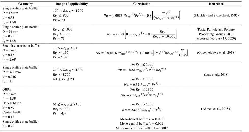
Table 2.4: Correlations for tube-side Nusselt number found the literature. ... 24
Table 2.5: Mean droplet size correlations for oscillatory baffled reactors. ... 30
Table 2.6: Scale-up correlations forms found the literature. ... 34
Table 2.7: Examples of OBR applications ... 38
Table 4.1: Simulation conditions proposed. ... 81
Table 4.2: Characteristics of different meshes used for the mesh and time step independency study. . 84
Table 4.3: Quantification of the effect of body mesh, inflation layers and time step on the axial velocity and pressure at different monitor points (M0-M3) with the MADP. ... 85
Table 4.4: Influence of the body mesh, inflation layers, time step and power calculation method on power dissipation and MADP values. ... 88
Table 4.5: Contribution of the individual terms of equation (4.10) on power dissipation 𝑃𝑀𝐸. ... 89
Table 5.1: Experimental conditions proposed by 2𝑘 factorial design. ... 100
Table 6.1: Operating conditions studied. ... 128
Table 6.2: Reactant concentrations. ... 129
List of figures
Figure 2.1: Schematic diagram of a continuous oscillatory baffled reactor with a single orifice plate baffles. ... 4 Figure 2.2: Van Dijck (1935) patent design of (a) reciprocating plate column, and (b) pulsed plate column. ... 5 Figure 2.3: Number of research publications on oscillatory flow from 1970 to 2019. Data obtained from Web of Science using the keywords “oscillatory flow reactor”. ... 6 Figure 2.4: Eddy formation in oscillatory baffled reactor (McDonough et al., 2015) ... 6 Figure 2.5: Axial to radial velocity ratio (RV) as function of oscillatory Reynolds number for different fluids (green and white legend in the plot refer to low and high viscosity non-Newtonian fluids, respectively) (Manninen et al., 2013). ... 16 Figure 2.6: The dependency of the tanks-in-series model parameter, 𝑁, on the oscillatory Reynolds number for different net Reynolds (Ni et al., 2003b). ... 17 Figure 2.7: Influence of oscillatory conditions and baffle geometry on the mean shear strain rates (Mazubert et al., 2016b). ... 20 Figure 2.8: Heat transfer enhancement in oscillatory baffled tubes (Ni et al., 2003b). ... 21 Figure 2.9: 𝑘𝐿𝑎 against power density for a single orifice baffle 50 mm OBR and a STR at constant superficial gas velocity (Hewgill et al., 1993). ... 27 Figure 2.10: (a) mean droplet size as function of oscillatory velocity, with 𝐴 = 𝑥𝑜, (b) droplet size distribution for different net flowrate and same oscillatory conditions (𝑥𝑜 = 52 mm and 𝑓 = 1.17 Hz) (Lobry et al., 2013). ... 29 Figure 2.11: Comparison of power density and length to diameter ratio behaviour for OBRs and turbulent flow reactor (Stonestreet and Harvey, 2002). ... 35 Figure 3.1: Overview of the Pressure-Based Solution Methods (a) Segregated algorithm (b) Coupled algorithm (ANSYS Inc., 2019). ... 65 Figure 3.2: Non-Iterative Time Advancement Solution algorithm (ANSYS Inc., 2019). ... 67 Figure 3.3: Control volume definition (a) cell-centred formulation, (b) vertex-centered formulation (Acharya, 2016). ... 69 Figure 3.4: Illustration of spatial discretization of the control volume defined by Fluent ANSYS (ANSYS Inc., 2019). ... 70 Figure 3.5: One-dimensional control volumes showing cell locations used in the QUICK scheme (ANSYS Inc., 2019). ... 70 Figure 3.6: Illustration of spatial discretization of the control volume defined In ANSYS CFX (ANSYS Inc., 2017). ... 72 Figure 4.1: (a) Photograph of the NiTech® COBR and (b) the geometry of the COBR simulated by CFD. ... 80 Figure 4.2: Example of tetrahedral mesh and inflation layers employed. ... 82 Figure 4.3: Locations of the monitor points and lines. M0: tube centerline, 8.45 mm upstream of the first orifice. M1 & L1: tube centerline, 8.45 mm upstream of the third orifice. M2: tube centerline, in the third orifice of the geometry. M3 & L2: tube centerline, at 8.45 mm downstream of the third orifice. 82 Figure 4.4: Images of the meshes used for the mesh and time step independency study: (a) Mesh 1, (b) Mesh 2, (c) Mesh 3, (d) Mesh 4, (e) Mesh 5. ... 83 Figure 4.5: Comparison between power dissipation calculation methods for the three different mesh sizes. ... 86
Figure 4.7: Power dissipation profiles determined via the integral of viscous dissipation at L2 as a
function of the radius for three different numbers of inflation layers at t/T = 0.60. ... 87
Figure 4.8: Comparison between power dissipation calculation methods for different time steps. ... 89
Figure 4.9: Power density as function of 𝑅𝑒𝑜. ... 90
Figure 4.10: Power density as a function of velocity ratio (𝜓). ... 91
Figure 4.11: Power density as function of 𝑅𝑒𝑇. ... 93
Figure 4.12: Dimensionless power density as a function of 𝑅𝑒𝑇. ... 94
Figure 5.1: Geometry of the COBR simulated by CFD with the location of tracer sources and monitoring planes. ... 99
Figure 5.2: Radial variation of (a) axial velocity and scalars released (b) at the axis (Source 0) and (c) mid-baffle (Source 1) at one quarter of the time through the first period for Case 1. The legend gives the mesh size in microns. ... 103
Figure 5.3: Velocity vectors during the oscillatory flow for Case 5 (𝑅𝑒𝑛𝑒𝑡 = 6, 𝑓 = 1 Hz, 𝑥𝑜 = 5 mm): (a) t/T = 0.00, (b) t/T = 0.25, (c) t/T = 0.55, (d) t/T = 0.6, (e) t/T = 0.75, (f) t/T = 0.95, (g) normalized inlet velocity over an oscillatory period for Case 5 with the representation of the positions of the different times t/T during the period. ... 105
Figure 5.4: Effect of source position on tracer patterns over a flow period (𝑇) for Case 1 (𝑅𝑒𝑛𝑒𝑡 = 27, 𝑓 = 1 Hz, 𝑥𝑜 = 5 mm): (a) Source 0, (b) Source 1, (c) Source 2... 107
Figure 5.5: Tracer profiles from Source 2 over a flow period (𝑇) at Plane 4 for Case 1 (𝑅𝑒𝑛𝑒𝑡 = 27, 𝑓 = 1 Hz, 𝑥𝑜 = 5 mm). ... 108
Figure 5.6: Areal distribution of mixing intensity averaged over one oscillation period at Plane 4 for Source 1: (a) Case 1, (b) Case 2, (c) Case 3, (d) Case 4, (e) Case 5, (f) Case 6, (g) Case 7, (h) Case 8. ... 109
Figure 5.7: Areal distribution of mixing intensity averaged over one oscillation period at Plane 4 for Source 2: (a) Case 1, (b) Case 2, (c) Case 3, (d) Case 4, (e) Case 5, (f) Case 6, (g) Case 7, (h) Case 8. ... 110
Figure 5.8: Area fraction of Planes 1, 2, 3, and 4 (averaged over one oscillation period) where > 90% mixing is achieved for Cases 1 to 8. (a) Source 0; (b) Source 1; (c) Source 2. ... 113
Figure 5.9: Tracer patterns over a flow period (𝑇) for Case 7 (𝑅𝑒𝑛𝑒𝑡 = 6, 𝑓 = 2 Hz, 𝑥𝑜 = 5 mm): (a) Source 0, (b) Source 1, (c) Source 2. ... 114
Figure 5.10: Tracer patterns over a flow period (𝑇) for Case 8 (𝑅𝑒𝑛𝑒𝑡 = 6, 𝑓 = 2 Hz, 𝑥𝑜 = 10 mm): (a) Source 0, (b) Source 1, (c) Source 2. ... 115
Figure 5.11: Area fraction of Planes 4 (averaged over one oscillation period) where > 90% mixing is achieved as a function of the power dissipation. (a) Source 0; (b) Source 1; (c) Source 2. ... 117
Figure 6.1: Photograph of the baffles in the NiTech® COBR ... 123
Figure 6.2: (a) Schematic diagram of the experimental setup containing the Nitech® reactor R-01. V-01 to V-03 are valves, FV-01 and FV-02 are feed vessels, P-01 to P-03 are gear pumps, F-01 is the flowmeter and SV-01 is the sample vessel. (b) Schematic diagram of the entries from P-01 (bulk flow), P-02 (side injection flow) and P-03 (oscillatory flow) to the Nitech® reactor. ... 124
Figure 6.3: Photograph of the presence of iodide (𝐼2) in the experiments without oscillations, with an acid concentration 𝐻2𝑆𝑂4 = 1 mol L–1. ... 130
Figure 6.4: Absorption spectra obtained for experiments without oscillations using an acid concentration 𝐻2𝑆𝑂4 = 1 mol L–1. ... 131
Figure 6.6: Example curve of segregation index as function of the calculated micromixing time for 𝑅 = 7 and [𝐻2𝑆𝑂4] = 0.015 mol L–1. ... 133 Figure 6.7: Segregation index as function of oscillatory Reynolds number for 𝐻2𝑆𝑂4 = 0.015 mol L–1, 𝑅 = 7 and 𝑅𝑒𝑛𝑒𝑡 = 125. ... 135 Figure 6.8: Segregation index as function of oscillatory Reynolds number for different acid flow rates. ... 136 Figure 6.9: Schematic diagram of the acid-buffer contacting zone; the grey zone is the volume used for the calculation of specific power density. ... 137 Figure 6.10: Segregation index as function of the specific power density. Dashed lines denote the positive and negative deviation from the trendline (solid line): ±50%. Open symbols correspond to acid concentration [𝐻2𝑆𝑂4] = 0.015 mol L–1 and 𝑅 = 7; filled symbols correspond acid concentration [𝐻2𝑆𝑂4] = 0.0075 mol L–1 and 𝑅 = 3.5. Symbol shapes represent the operatory conditions: (𝑥𝑜 = 0 𝑚𝑚, 𝑓 = 0 𝐻𝑧, 𝑅𝑒𝑜 = 0), (𝑥𝑜 = 3 𝑚𝑚, 𝑓 = 1.5 𝐻𝑧, 𝑅𝑒𝑜 = 400), (𝑥𝑜 = 4.5 𝑚𝑚, 𝑓 = 1 𝐻𝑧, 𝑅𝑒𝑜 = 400), (𝑥𝑜 = 6.5 𝑚𝑚, 𝑓 = 1 𝐻𝑧, 𝑅𝑒𝑜 = 600), (𝑥𝑜 = 13 𝑚𝑚, 𝑓 = 0.5 𝐻𝑧, 𝑅𝑒𝑜 = 600), (𝑥𝑜 = 13 𝑚𝑚, 𝑓 = 1 𝐻𝑧, 𝑅𝑒𝑜 = 1200) and (𝑥𝑜 = 13 𝑚𝑚, 𝑓 = 1.5 𝐻𝑧, 𝑅𝑒𝑜 = 1800). ... 138 Figure 6.11: Theoretical (dash-dotted line) and calculated (open/filled symbols) micromixing time as function of the specific power density. Dashed lines denote the positive and negative deviation from the trendline (solid line): ±40%. Open symbols correspond to acid concentration [𝐻2𝑆𝑂4] = 0.015 mol L– 1 and 𝑅 = 7; filled symbols correspond acid concentration [𝐻2𝑆𝑂4] = 0.0075 mol L–1 and 𝑅 = 3.5. 139 Figure 6.12: Schematic diagram of the entries from 01 (bulk flow), 02 (side injection flow) and P-03 (oscillatory flow) to the Nitech® reactor. ... 142 Figure 6.13: Images for the different inlets orientations: (a) top entry, (b) bottom entry. Blue tube feed the bulk flow, and the red tube feed the secondary injection – the distance between the tubes is 30 cm. ... 142 Figure 6.14: Tracer patterns for (a) Case 1 and (b) Case 2. ... 143 Figure 6.15: Results of the central passive injection for the inlets top entry orientation using water as the working fluid. ... 146 Figure 6.16: Results of the central passive injection for the inlets bottom entry orientation using water as the working fluid. ... 148 Figure 6.17: Results of the central passive injection for the inlets bottom entry orientation using a solution of 69% wt. glycerol/water as the working fluid. ... 151 Figure 6.18: Inlet zone between the net flow (blue pipe) and the system, with the oscillations being provided through the white pipe. ... 151
Nomenclature
𝐴 OBR cross-section area (m-2)
𝐴𝑡 actual value at time 𝑡
𝐶 species concentration (kg m-3)
𝐶∗ dimensionless tracer concentration (-)
𝐶𝑖 local scalar concentration of the tracer at the time 𝑡 (kg m-3)
𝐶𝑖∗ local dimensionless tracer concentration at the time t (-)
𝐶𝑖 molar concentration of ion 𝑖 (mol L-1)
𝐶̅ fully mixed concentration (kg m-3) 𝐶𝐷 orifice discharge coefficient (-)
𝐶0 concentration of tracer in the injection source (kg m-3)
𝐶𝑜 Courant number, 𝑣 ∆𝑡 ∆𝑥⁄ (-) 𝐶𝑝 fluid specific heat (J kg-1 K-1)
𝐶𝑋− lower limit of mixedness ranges (-)
𝐶𝑋+ upper limit of mixedness ranges (-)
𝑐𝑖 10 concentration of the specie 𝑖 in the surrounding fluid (mol L-1)
𝐷 OBR diameter (m)
𝑑 OBR orifice diameter (m)
𝐷𝑎𝑥 axial dispersion coefficient (m2 s-1)
𝐷𝑓 diffusion coefficient (m2 s-1)
𝐷ℎ hydraulic diameter (m)
𝑑32 Sauter mean diameter (m)
𝑑𝑣,0.5 mean particle size (m)
𝐹𝑡 forecast value at time 𝑡
𝑓 oscillation frequency (Hz)
𝑓𝑠 frequency of vortex shedding (Hz)
ℎ𝑂𝐵𝑅 OBR-side transfer coefficient (W m-2 K-1)
𝐼 ionic strength (mol L-1)
𝐾𝐵 Equilibrium constant of reaction (R3)
𝑘1 reaction rate coefficient of reaction (R1) (L mol-1 s-1)
𝑘2 reaction rate coefficient of reaction (R2) (mol-4 s-1)
𝑘3𝑓 reaction rate coefficient of reaction (R3)
𝑘3𝑏 reaction rate coefficient of reaction (R3)
𝑘𝐿 liquid-side mass transfer coefficient (m s-1)
𝑘𝐿𝑎 volumetric mass transfer coefficient (s-1)
𝑙 mixing length (m)
𝑙 optical path length (m)
𝑙∗ mixing length proposed by Jimeno et al. (2018b) (m)
𝑙𝑏 distance between baffles (m)
𝑙𝑏𝑜𝑝𝑡 optimum distance between baffles (m)
𝐿 reactor length (m)
𝑛 number of baffles (-)
𝒏 normal vector (-)
𝑛̇ molar flow rate (mol m-3)
𝑁 number of theorical baffles (-)
𝑁𝑢 Nusselt number (-)
𝑂𝐷 optical density or light absorption (-)
𝑝 pressure (Pa)
𝑃 power dissipation (W)
𝑃𝑟 Prandtl number (𝐶𝑝𝜇⁄ ) (-) 𝑘
𝑃𝑉𝐷 power dissipation calculated using the viscous dissipation equation (W)
𝑃𝑀𝐸 power dissipation calculated using the mechanical energy equation (W)
𝑃/𝑉 power density (W m-3)
(𝑃/𝑉)∗ dimensionless power density (-)
𝑃𝑒 Péclet number (-)
𝑞̇ volumetric flow rate (m3 s-1)
𝑞 volumetric flow rate at the tracer inlet (m3 s-1) 𝑞𝑗𝑒𝑡 volumetric flow rate of the side injection (m3 s-1)
𝑄 volumetric flow rate at the COBR inlet (m3 s-1) 𝑄𝑛𝑒𝑡 volumetric flow rate of the main stream (m3 s-1)
𝑅 radius of reactor (m)
𝑅 volumetric flow rate ratio between the bulk and jet stream (-) 𝑅𝑉 axial to radial velocity ratio (-)
𝑅𝑒𝐺 net flow Reynolds number for gas (-)
𝑅𝑒𝑛𝑒𝑡 net flow Reynold number (-)
𝑅𝑒𝑜 oscillatory Reynolds number (-)
𝑅𝑒𝑜′ modified oscillatory flow Reynolds number proposed by Ahmed et al. (2019) (-)
𝑅𝑒𝑇 total Reynolds number proposed by Jimeno et al. (2018b) (-) 𝑟 radial coordinate (m) 𝑟𝑛 radial number (-) 𝑆 surface (m2) 𝑺 surface vector (m2) 𝑆𝑐 Schmidt number (-)
𝑆̇𝐶 mass source of tracer (kg m-3 s-1)
𝑆ℎ Sherwood number (-) 𝑆𝑛 swirl number (-) 𝑆𝑡 Strouhal number (-) ∆𝑡 time step (s) 𝑡 time (s) 𝑡𝑚 micromixing time (s)
𝑡𝑚 𝑡ℎ𝑒𝑜 theoretical micromixing time considering only the molecular diffusion (s)
𝑡𝑚 𝑐𝑎𝑙 calculated micromixing time (s)
𝑇 oscillation period (s)
𝑢 instantaneous velocity (m s-1)
𝒖 velocity vector (m s-1)
𝑢̅ mean velocity (m s-1)
𝑢𝑔 superficial gas velocity at standard pressure (m s-1)
𝑢𝑖𝑛 initial velocity (m s-1)
𝑢𝑖,𝑎𝑥𝑖𝑎𝑙 axial velocity in computational cell 𝑖 (m s-1)
𝑢𝑖,𝑡𝑟𝑎𝑛𝑠𝑣𝑒𝑟𝑠𝑒 transverse velocity in computational cell 𝑖 (m s-1)
𝑢𝑛𝑒𝑡 net velocity (m s-1)
𝑢𝑥, 𝑢𝑦, 𝑢𝑧 velocity components (m s-1)
𝑉 volume (m3)
𝑉2 volume of the aggregate (m3)
𝑉20 initial value of the aggregate volume (m3)
𝑣𝑟 radial velocity (m s-1)
𝑣𝑧 axial velocity (cylindrical coordinate) (m s-1)
𝑣𝜃 tangential velocity (m s-1)
𝑥𝑜 oscillation amplitude (m)
𝑊𝑒ℎ hydrodynamic Weber number (-)
𝑊𝑒𝑠 Weber number (-)
𝑋 percentage of perfectly-mixed state (-)
𝑥, 𝑦, 𝑧 cartesian coordinates (m)
𝑌 selectivity of the iodide reaction (-)
𝑌𝑇𝑆 selectivity of iodide when there is total segregation (-)
𝑧𝑖 charge number of species i (-)
Greek symbols
𝛼 dimensionless free baffle area (𝑑 𝐷⁄ )2(-) 𝛽 optimal to use baffle spacing ratio (-)
𝛤 relevant effective diffusivity coefficient (m2 s-1)
𝛾̇ mean shear rate (s-1)
𝛿 baffle thickness (m)
𝜹 unit tensor (-)
𝛿0 initial striation thickness (m)
𝜀 specific power density per mass (W kg-1)
𝜀 molar extinction coefficient of 𝐼3− ions at 353 (L mol-1 cm-1)
𝜅 dilatational viscosity (Pa.s)
𝝀 number of time steps in an oscillatory cycle (-)
𝜆 coefficient of thermal performance by Ahmed et al. (2018a) (-)
𝜇 dynamic viscosity (Pa.s)
𝜌 fluid density (kg m-3)
𝞼 momentum flux tensor (Pa)
τ theoretical residence time (s)
𝛕 shear stress vector (Pa)
𝜐 kinematic viscosity (m2 s-1)
𝜙 scalar quantity variable (-)
𝝓 flux tensor (Pa)
Φ𝑣 dissipation function (s-2)
𝜑 correction factor (-)
𝜓 velocity ratio (-)
List of publications
Journal papers
Avila, M., Fletcher, D.F., Poux, M., Xuereb, C., Aubin, J., 2020. Mixing performance in continuous oscillatory baffled reactors. Chem. Eng. Sci. 219. https://doi.org/10.1016/j.ces.2020.115600
Avila, M., Fletcher, D.F., Poux, M., Xuereb, C., Aubin, J., 2020. Predicting power consumption in continuous oscillatory baffled reactors. Chem. Eng. Sci. 212.
https://doi.org/10.1016/j.ces.2019.115310
Conference posters
M. Avila, M Poux, C Xuereb, D. Fletcher, Joelle Aubin. Characterization of micromixing in a Continuous Oscillatory Baffled Reactor. 16th European Conference on Mixing, September 2018, Toulouse, France.
M. Avila, M Poux, C Xuereb, D. Fletcher, Joelle Aubin. Macro- and micro-mixing performance in continuous oscillatory baffled reactors. 6th European Process Intensification Conference, October 2017, Barcelona, Spain
Chapter 1. Introduction
The stirred tank reactor (STR) remain the standard approach for mixing and carrying out chemical reactions from early stage discovery to manufacture. Many areas of chemical and process industries are still dependent on this kind of reactors at plant scale. The most definite advantage of batch production is the lower initial setup cost (although this is not always true). However, continuous processing is becoming a more viable option for these industries due to advancements in design and technology. Compared with continuous processing, STR is much slower, increasing the overall cost of processing. Starting up and using batch equipment can also increase energy consumption and the quality discrepancy between batches may differ. This can lead to lost production and compromised quality if the batch process is not monitored closely and properly. Many industrial sectors are shifting from traditional batch processes to continuous processes.
For most applications, a continuous process saves time, energy, and costs and when implemented correctly, it can offer much faster operation, reduce waste, improve quality, increase productivity and adapt to the needs of customers more efficiently than batch processing. Continuous processes usually require less space than batch processes. Significant reductions in dimensions leads to high efficiency in mass and heat transfer: smaller volume means larger heat exchange surface, shorter residence time and much easier control of the process.
The transition from batch to continuous operation, aiming to reduce reactant volume and miniaturization in dimensions is an example of process intensification. Process intensification (PI) is defined as drastic improvements in chemical manufacturing and processing; substantially decreasing equipment volume, energy consumption, or waste formation; ultimately leading to cheaper, safer and sustainable technologies (Stankiewicz and Moulijn, 2000)1. According to Stankiewicz and Moulijn, process intensification can be divided into two areas. The first is the process intensifying equipment, which are special designs that optimize critical parameters (e.g., heat transfer, mass transfer), such as novel reactors, and intensive mixing, heat-transfer and mass-transfer devices. The second area is the process intensifying methods, where multiple processing steps are integrated into a single unit operation (as hybrid separations, integration of reaction and separation, heat exchange, or phase transition), or alternative energy sources are used (light, ultrasound, etc.), and new process-control methods (such as intentional unsteady-state operation). Some examples of process intensifying equipment are spinning disk reactors, rotating packed bed, microreactors, rotor-stator devices, static mixers, compact heat exchangers, and oscillatory baffled reactors.
An oscillatory baffled reactor (OBR) is a particular type of tubular reactor, which has drawn increasing attention over the past few decades. Eddy generation due to an oscillatory flow and their
1
Stankiewicz, A.I., Moulijn, J.A., 2000. Process Intensification: transforming chemical engineering. Chem. Eng. Prog. 96, 22–34.
interaction with internal baffles characterize the OBR. This intensified reactor has proven to globally intensify processes when compared with STRs. OBRs have been applied in several industrial sectors. However, despite being already used for industrial production, this equipment presents some limitations and today is being studied to be implemented in a wider range of operation conditions and industrial sectors.
In this context, a review of this intensified technology is presented in the next chapter, highlighting its characteristics, process enhancements, applications and the limitations found in the literature. The aim is to analyse and identified new areas of opportunities that will allow this technology to be applied in a broader range of applications for continuous processing.
Chapter 2. Literature review
This chapter focuses on a review of the OBR technology and its limitations that motivate this thesis work. The chapter is divided into two parts: Part I presents the state of the art of the most important characteristics of the OBR. Part II highlights the motivation of the research, along with the general objective and the thesis structure.
Part I: Oscillatory baffled reactors: characterisation, applications and limitations –
state of the art
2.I.1. Introduction
The development of green and sustainable technologies is of prime importance for the chemical and process industries due to increasing social and environmental concerns. One of the major challenges that these industries face currently is the creation of innovative processes for the production of commodity and intermediate products that allow high product quality with specified properties and that are less polluting, as well as more efficient in terms of energy, raw materials and water management.
Stirred tank reactors (STR) and continuous stirred tank reactors (CSTR) are widely used at the industrial scale in chemical and process industries, due to their simplicity and the extensive knowledge of these reactors. Continuous processing offers many benefits over batch operation, as it minimizes waste (Schaber et al., 2011), reduces energy consumption (Yoshida et al., 2011), improves mass and heat transfer (Singh and Rizvi, 1994; Yu et al., 2012), as well as chemical conversion (Hartman et al., 2011). One of the main aims in continuous processing is the design of chemical reactors that enable plug flow. Tubular reactors offer good mixing performance and plug flow under turbulent flow conditions, however, they require long tube lengths to achieve long residence times, resulting in high-pressure drop along the reactor. Nowadays, new technologies and devices have been developed to achieve plug flow in more compact geometries, such as static in-line mixers, packed bed reactors, microreactors and oscillatory baffled reactors. In the plug flow state the fluid is perfectly mixed in the radial direction but not in the axial direction (forwards or backwards).
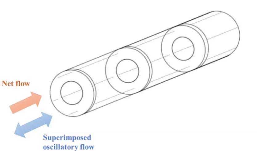
The oscillatory baffled reactor (OBR) is a particular type of tubular reactor, typically equipped with periodically spaced sharp-edged orifice baffles along its length, as is shown in Figure 2.1. This type of reactor operates with a periodic oscillatory or pulsed flow, which with the presence of the baffles, causes unsteadiness in the laminar flow. The oscillations are normally generated by diaphragms, bellows or pistons at one or both ends of the tube. This technology has been called pulsed flow reactor (PFR), oscillatory baffled column (OBC), or oscillatory baffled reactor (OBR) in the literature. In this chapter, the expression OBR is used to cover batch processes and continuous flow.
Figure 2.1: Schematic diagram of a continuous oscillatory baffled reactor with a single orifice plate baffles.
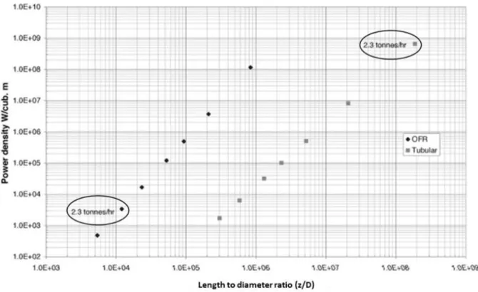
Due to the interaction of fluid pulsations with the baffles and the resulting recirculating flow (see section 2.I.2.1 for details), mixing in OBRs is independent of the net flow when operated continuously, providing a good mixing quality and long residence times (comparable with those obtained in batch reactors) with a greatly reduced length-to-diameter ratio tube (Harvey et al., 2003). Due to these characteristics, OBRs have proven to globally intensify processes, leading to operations that use less energy and produce less waste compared with processes in conventional STRs (Phan et al., 2011a; Reis et al., 2006b).
The idea of pulsed flow reactors is not new. The first apparition of oscillation conditions for industrial applications was the patent of Van Dijck (1935). The patent, as illustrated in Figure 2.2, describes vertical pulsed and reciprocating plate columns for liquid-liquid extractions that are equipped with oscillating perforated sieve plates or with immobile internals. Until the 1980s, the pulsed packed column (Baird and Garstang, 1972; Burkhart and Fahien, 1958) and reciprocating plate column (Karr, 1959), were the only equipment using oscillatory flow for enhancing heat and mass transfer. The pulsation of the fluid and the reciprocating plates have both shown to improve the dispersion of liquid phases and increase the interfacial area, providing enhanced mass transfer performance compared with conventional extraction columns. In the 1980s, the interest in the details of periodic flows increased due to the improvement of mass and heat transfer offered by oscillatory flow mixing. Knott and Mackley (1980) studied the nature of the eddies created at the sharp-edge channels under the influence of periodic flows and observed the formation and separation of vortex rings, which were explained to be the origin of the enhanced transport phenomena. Following this, a number of pioneering studies were conducted. Howes (1988) investigated the dispersion of a passive tracer in both batch and continuous OBRs and concluded that net flow, amplitude and frequency affects the axial dispersion of the passive tracer. Increasing the oscillatory velocity (i.e. 𝑓. 𝑥𝑜) increases radial mixing, thereby decreasing axial dispersion. By increasing net flow, backmixing is decreased. However, for low oscillatory velocities, the net flow will increase axial dispersion since the radial mixing to counterbalance the effects of net flow. Brunold et al. (1989) studied the influence of oscillatory flow on the flow patterns in a duct
containing sharp edges. Their experimental flow observations describe the formation, development and separation of large-scale eddies in the baffle area and were found to lead to efficient mixing. Later the same year, Dickens et al. (1989) experimentally characterized the mixing performance in a horizontal OBR under laminar net flow conditions via the measurement of the residence time distribution (RTD), reporting plug flow behaviour. Mackley et al. (1990) investigated heat transfer in OBRs. Their work showed a significant increase in heat transfer in the presence of oscillations with respect to the same mass flow rate in a classical tubular reactor. Their results also demonstrated that oscillatory flow and the sharp-edged orifice baffles must be present to produce this enhancement.
The interest in oscillatory flow has been increasing over the last forty years, and particularly since the 1990s where there has been a relatively steady increase over the years as can be seen in Figure 2.3. Since then, there have been more and more in oscillatory flow for enhancing the performance chemical reactors and new areas of research have emerged, such as combined microwave heating and OBRs for the production of a metal-organic frameworks (Laybourn et al., 2019), combined heat pipes and OBRs to performing exothermic reactions, which operate through the evaporation and condensation of a working fluid (McDonough et al., 2018, 2016), as well as the development of crystallization processes using moving baffle oscillatory reactors (Raval et al., 2020).
(a) (b)
Figure 2.3: Number of research publications on oscillatory flow from 1970 to 2019. Data obtained from Web of Science using the keywords “oscillatory flow reactor”.
2.I.2. Flow and reactor design
2.I.2.1. Description of flow
The overall mechanism of eddy formation in OBRs has been described widely in the literature (Brunold et al., 1989; Gough et al., 1997; Mazubert et al., 2016a; McDonough et al., 2015; Ni et al., 2002). Typical flow patterns formed in OBRs with orifice baffles are shown in Figure 2.4. During the flow acceleration phase (Figure 2.4(a)), eddies are formed downstream of the baffles and flow separation starts. As the oscillatory velocity increases ((Figure 2.4(b)), eddies start to fill the baffle cavity. At the flow reversal phase (Figure 2.4(c)), the eddies are detached from the baffle, leaving a free vortex that is engulfed by the bulk flow and that interacts with other vortices that were generated in previous cycles (Figure 2.4(d)), before restarting the cycle again.
2.I.2.2. Geometries and configurations
Sharp-edged single orifice baffles (as shown in Figure 2.1) are the most common baffle design used in OBR studies, however there are a number of other baffle geometries that have been studied in the literature. These geometries are shown in Table 2.1 and include periodic smooth constrictions, multi-orifice plates, disc-and-doughnuts, helical forms (round wires, sharp-edged and alternating ribbon, double ribbons, combined with a central rod), central disc baffles, and wire.
Periodic smooth constrictions are based on the single orifice plate baffle design. The main difference is that orifices in smooth constriction baffles are made by constricting the reactor tube (usually made with glass) and hence offers low and uniform shear rates, which may be advantageous for applications such as shear-sensitive bioprocesses (Reis et al., 2006a, 2006b).
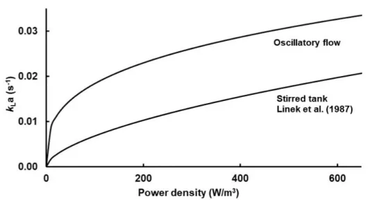
Multi-orifice designs are the same as those in the pulsed and reciprocating multi-orifice plate columns. This geometry is attractive due to the ease of manufacture. The influence of the number of orifices was studied by González-Juárez et al. (2017) using numerical simulations. A higher number of orifices enhance radial mixing, thanks to the production of a larger number of small eddies. With a significant number of orifices, the reactor achieves narrower RTD curves with a more uniform concentration in the cross-section, thus improving the plug flow behaviour and the mixing quality. Ahmed et al. (2018b) studied mass transfer in air-water systems for different OBR geometries and concluded that the multi-orifice design is recommended over the smooth constrictions, single orifice and helical baffle geometries for gas-liquid mass transfer applications. Indeed, the multi-orifice geometry offers better control of the size and shape of the bubbles and microbubbles, offering a wider bubbly flow region and higher volumetric mass transfer coefficient than the other geometries.
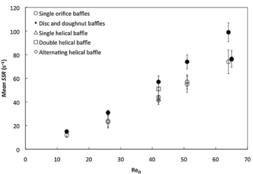
In the disc-and-doughnut geometry, the disc placed between the orifice plate acts as a barrier to the axial flow, generating additional radial flow. This design has been used largely in liquid-liquid extraction columns for a long time (Al Khani et al., 1988; Angelov et al., 1990; Laulan, 1980; Leroy, 1991; Martin, 1987) and its geometry has been employed in pulsed liquid-liquid dispersion operation (Lobry et al., 2013; Mazubert et al., 2016a). Mazubert et al. (2016a, 2016b) studied the disc-and- doughnut geometry and they found that this geometry shows the highest values of shear strain rates, pressure drop and energy dissipation (important parameters for multiphase flow applications) when compared with other geometries, such as the single orifice plate, single helical ribbon, double helical ribbon and alternating helical ribbon. However, this design does not improve radial mixing or decrease axial dispersion in comparison with the single orifice baffle.
Helical baffles have been shown that this geometry enables plug flow behaviour to be achieved over a wider range of oscillatory conditions than other geometries, due to additional “swirl motion” that is created from the interactions of the oscillatory flow and the helical baffle (Phan and Harvey, 2011a, 2010). This swirl flow has been identified by different authors using numerical simulation (Mazubert et al., 2016a, 2016b; Solano et al., 2012) and PIV experiments (McDonough et al., 2017). Different variations of this geometry exist, each one having specific properties and characteristics. There are
helical baffles made simply by coiling round wire, as well as sharp-edged helical baffles, alternating helical ribbons and double helical ribbons, which are variants using a coiled blade or ribbon. The sharp-edged helical baffle has shown to provide better yield in the production of biodiesel than the coiled wire helical baffle, due to the sharp baffle edge, which generates higher shear rates and enables more effective liquid-liquid phase mixing (Phan et al., 2011b). The alternating helical ribbon consists of a single blade that revolves in different directions every two periods, and in the double helical ribbon the blades revolve in opposite directions. The vortical flow is less apparent in the alternating helical blade, and streamlines appear to occupy less volume in the reactor, suggesting that flow turnover close to the walls is less efficient (Mazubert et al., 2016a). The helical baffle and alternating helical baffle provide improved plug flow behaviour compared with that generated by the single orifice and the disc-and-doughnut baffles (Mazubert et al., 2016a, 2016b). These authors also conclude that helical baffles provide lower axial dispersion, whilst maintaining significant levels of shear strain rate.
Axial circular baffles (or central baffles) are periodically spaced discs mounted on an axial rod. This geometry offers higher shear rates and pressure drop compared with the single baffle orifice and smooth constriction geometries (Ahmed et al., 2018a), making it useful for homogeneous liquid-liquid reactions (Rasdi et al., 2013; Yussof et al., 2018). The wire wool and sharp-edge helical blade with central rod geometries have also proven enhanced dispersion in liquid-liquid operations (Phan et al., 2012, 2011b). The helical coil baffle with central rod has been studied by McDonough et al. (2019a) using numerical simulation and comparing the results with PIV experiments. The presence of the central rod creates a new dual counter-rotating vortex regime, due to the significant swirl velocity generated by the helical coils.
Table 2.1: Different baffled geometries used in OBRs.
Baffled design Reference Single baffle orifice (plate)
(Mazubert et al., 2015; Ni et al., 2003a, 1998a; Stonestreet and
Van Der Veeken, 1999)
Single orifice (smooth constrictions)
(Ahmed et al., 2018b; Eze et al., 2013; Phan and Harvey, 2010;
Multi-orifice plate baffle
(Ahmed et al., 2018b; González-Juárez et al., 2017; Lucas et al., 2016; Palma and Giudici, 2003;
Smith and Mackley, 2006)
Disc-and-doughnut baffle
(Amokrane et al., 2014; Lobry et al., 2013; Mazubert et al., 2016a,
2016b)
Helical baffle
(Ahmed et al., 2018b; McDonough et al., 2019b, 2017;
Phan and Harvey, 2011a, 2010)
Sharp-edged helical baffle
(Mazubert et al., 2016a, 2016b; Phan et al., 2011b; Phan and
Harvey, 2011b)
Double helical baffle
(Mazubert et al., 2016a, 2016b)
Alternating helical ribbon
Central baffle
(Ahmed et al., 2018a; McDonough et al., 2019b; Phan et
al., 2011a; Phan and Harvey, 2010)
Wire wool
(Phan et al., 2012)
Sharp-edged helical with central rod
(Akmal et al., 2020; Phan et al., 2012, 2011b)
Helical baffle with central rod
(Horie et al., 2018; McDonough et al., 2019a)
2.I.2.3. Geometrical parameters
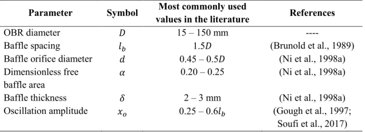
The geometrical parameters influence the shape and size of the generated vortices, which require adequate space to fully expand and spread in each baffle cavity. The main geometrical parameters in the design of oscillatory baffled reactors are based on the single orifice baffle design and are summarized in Table 2.2 and illustrated in Table 2.1. Table 2.2 gives the ranges of the most commonly used values, which were defined by the cited studies and are now often used as a design guideline. However, it should be pointed out that these ranges of values were defined for specific conditions used in the original studies and have never been optimised for a wide range of operating conditions or applications.
The selection of the OBR diameter depends on the process application and the desired production rate. In the literature, the conventional OBR diameter range is from 15 mm to 150 mm. However, it can be pointed out continuous flow OBRs offers the advantage of being able to ensure industrial-scale production even with 15 mm diameter reactors (Mazubert et al., 2015, 2014). In recent years, the interest in miniaturized OBRs (referred to meso-OBRs in literature) has increased. These miniaturized reactors
have diameters of ≤ 5 mm and they are typically operated with lower flow rates than the larger-scale OBRs, allowing reduced material inventory, as well as wastes generated in the process. These characteristics are particularly beneficial for rapid process screening and process development as explained by McDonough et al. (2015). Recent works show the feasibility of the use of meso-OBR as a reactor for multiphase reactions, such as solid-liquid carboxylic acid esterification (Eze et al., 2017), hexanoic acid esterification (Eze et al., 2013), as well as gas-liquid ozonation of water and wastewater (Lucas et al., 2016).
Table 2.2: Summary of main geometrical parameters in oscillatory baffled reactor design.
Parameter Symbol Most commonly used
values in the literature References
OBR diameter 𝐷 15 – 150 mm ----
Baffle spacing 𝑙𝑏 1.5𝐷 (Brunold et al., 1989)
Baffle orifice diameter 𝑑 0.45 – 0.5𝐷 (Ni et al., 1998a)
Dimensionless free baffle area
𝛼 0.20 – 0.25 (Ni et al., 1998a)
Baffle thickness 𝛿 2 – 3 mm (Ni et al., 1998a)
Oscillation amplitude 𝑥𝑜 0.25 – 0.6𝑙𝑏 (Gough et al., 1997;
Soufi et al., 2017)
The baffle spacing (𝑙𝑏) is a key design parameter in an OBR as it influences the shape and length of eddies within each baffle cavity (Brunold et al., 1989; Knott and Mackley, 1980). A good value of 𝑙𝑏 should ensure the full extension of the vortex generated behind the baffles, thus assuring its presence over the inter-baffle zone. Low values of baffle spacing cause the vortices to hit adjacent baffles before their full expansion, resulting in a constrained growth of eddies, a reduction of radial motion, as well as undesirable axial dispersion in continuous operations. For large values of baffle spacing, the vortices do not propagate through the full volume of the inter-baffle region. A spacing of 𝑙𝑏 = 1.5𝐷 has been the most commonly used value in the literature following the results reported by the flow visualizations of Brunold et al. (1989). Similar values have been recommended by others: Ni and Gao (1996b) reported a value of 𝑙𝑏 = 1.8𝐷 as the optimal in their studies of mass transfer, and Ni et al. (1998a) recommended a value of 𝑙𝑏 = 2𝐷 is needed to minimize the mixing time in a batch OBR with oscillating baffles. It should be mentioned that baffle spacing is also inherently related to oscillation amplitude and the effectiveness of eddy generation and mixing; this will be discussed later in this section.
The dimensionless free baffle area, defined as 𝛼 = (𝑑 𝐷⁄ )2, impacts the size of eddies generated in each baffle cavity. Small values of 𝑑 will constrict the fluid more as it flows through the baffles, resulting in larger vortices, and giving better mixing conditions. The dimensionless free baffle area is typically chosen in the range of 0.2–0.4 (Phan and Harvey, 2011b), but many studies have established a standardized orifice diameter of 𝑑 = 0.5𝐷 (Abbott et al., 2014a; Mackley and Stonestreet, 1995;
Navarro-Fuentes et al., 2019a; Ni et al., 1998a; Stonestreet and Harvey, 2002), which corresponds to a dimensionless free baffle area of 𝛼 = 0.25. Depending on if the flow is single or multi-phase, different values of 𝛼 may be preferred. Ni et al. (1998a) studied the effect of dimensionless free baffle area for single phase flow on the mixing time in OBRs using either oscillating baffles or pulsed flow, over a range of 0.11 < 𝛼 < 0.51. In both configurations (oscillating baffles and pulsed flow), shortest mixing times were achieved for values of 𝛼 = 0.20 − 0.22. In liquid-solid flows, Ejim et al. (2017) stated that the dimensionless free baffle area plays a dominant role in controlling solid backmixing and batch suspension of particles in meso-OBRs. In their study, a value of 𝛼 = 0.12 was found to minimize axial dispersion, resulting in a longer mean residence time of the solids.
Other geometrical parameters, such as the baffle thickness and the gap between baffle and wall, and their influence on mixing performance have also been reported. Ni et al. (1998a) studied the influence of baffle thickness on the mixing efficiency. Vortex generation is favoured by thinner baffles and they are deformed as the baffles get thicker. Thinner baffles are therefore recommended over thicker baffles, which will behave more like a step that a baffle. However, thinner baffles could negatively affect the mechanical stability of baffles, and it is expected that there would be a minimum baffle thickness to diameter ratio (𝛿 𝐷⁄ ) that ensures the stability of baffles and the vortex generation. The influence of the gap between the outer edge of the baffles and the tube wall on flow patterns has been studied using particle image velocimetry (PIV) (Ni et al., 2004a). It has been observed that an increased gap results in the generation of smaller eddies and an increase in the axial velocity, both leading to poor mixing performance. It is interesting to note that this study does not specify if the amount of tube cross-section open to flow was kept constant as the gap increased (i.e. by reducing the orifice diameter) or not. Indeed, this is expected to be an important parameter and for equal cross-sections open to flow, one can imagine higher axial dispersion to be obtained in geometries with no (or little) gap at the wall.
For fixed values of interbaffle spacing and orifice diameter, 𝑙𝑏 and 𝑑, the combination of amplitude and frequency controls the generation and the propagation of eddies, producing different fluid flow behaviour. Gough et al. (1997) studied the effect of the oscillation frequency and amplitude on flow pattern by qualitative flow visualization in polymerisation suspensions in a modified OBR. It is important to point out that in this study, fluid oscillation was achieved by oscillating the baffles and not the fluid. From this study, the oscillation amplitude required to achieve similar flow patterns at those presents in a conventional OBR (where the flow is pulsed) is approximately equal to 0.25𝑙𝑏 . Eventhough, the operation of the reactor used in Gough et al. (1997)’s study is rather different that both batch and continuous flow OBRs, this value of oscillation amplitude has been widely used for OBR design since that time. More recently, Reis et al. (2005) investigated a range of ratios of oscillation amplitude/baffle spacing, ranging from 0.015 to 0.85. It was shown that flow separation occurred with amplitude values lower than 0.25𝑙𝑏, the general recommendation. In an optimisation study carried out by Soufi et al. (2017), an amplitude value of 0.6𝑙𝑏 was found to give an optimal reaction yield in a mass
transfer limited liquid-liquid reaction that is significantly greater than the general design guideline. Indeed, these authors claim that the ‘optimal’ design of OBRs certainly depends on the type of application (single phase, gas-liquid, solid-liquid etc.), the process objective and the performance parameter that is being optimized.
The recommended values of geometrical parameters and the design guidelines for OBRs have mainly been based on the single orifice geometry and on the results of limited studies. It is clear that for some designs (e.g. helical baffles and wire meshes), these guidelines are for the most part not applicable or need some modification. For example, the multi-orifice plate baffle uses an equivalent diameter instead of the baffle orifice diameter to calculate the dimensionless free baffle area; helical baffles use the pitch (i.e. the axial distance of one complete helix turn) instead of the baffle spacing. Other geometries such as the disc-and-doughnut baffles have additional design parameters that need to be considered, such as the disc diameter and the distance between the disc and the orifice.
2.I.2.4. Dimensionless groups in continuous oscillatory flow
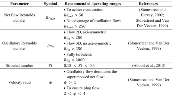
The key dimensionless groups that characterize the fluid mechanics and flow conditions in OBRs are the net flow Reynolds number (𝑅𝑒𝑛𝑒𝑡), oscillatory Reynolds number (𝑅𝑒𝑜), Strouhal number (𝑆𝑡), and velocity ratio (𝜓). These are presented in
Table 2.3 and described briefly below.
The net flow Reynolds number controls the flow regimes of the fluids (from laminar to turbulent flow), and is defined as the ratio of inertial forces to viscous forces:
𝑅𝑒𝑛𝑒𝑡=𝜌𝑢𝑛𝑒𝑡𝜇 𝐷 (2.1)
The oscillatory Reynolds number describes the intensity of mixing in the reactor. In 𝑅𝑒𝑜, the characteristic velocity is the maximum oscillatory velocity:
𝑅𝑒𝑜=2𝜋𝑓𝑥𝜇𝑜𝜌𝐷 (2.2)
Stonestreet and Van Der Veeken (1999) identified three different flow regimes: for 𝑅𝑒𝑜< 250 the flow is essentially 2-dimensional and axi-symmetric with low mixing intensity; for 𝑅𝑒𝑜 > 250 the flow becomes 3-dimensional and mixing is more intense; finally, when 𝑅𝑒𝑜> 2000, the flow is fully turbulent.
The Strouhal describes oscillating flow behaviour and is often defined as 𝑆𝑡 = 𝑓𝑠𝐷⁄ . However 𝑢 Brunold et al. (1989) adapted the equation to a baffled tube, following the flow patterns
numerically modelled and observed by Sobey (1980): 𝑆𝑡 =4𝜋𝑥𝐷
𝑜
(2.3)
This equation is the most used in OBR characterizations. The Strouhal number measures the effective eddy propagation with relation to the tube diameter. Higher values of 𝑆𝑡 promote the propagation of the eddies into the next baffle (Ahmed et al., 2017). The most common range of the Strouhal numbers used in the literature is 0.15 < 𝑆𝑡 < 4 (Abbott et al., 2013).
It should be pointed out that surprisingly the baffle spacing, 𝑙𝑏, which influences the shape and length of eddies within each baffle cavity, is absent in the definition of 𝑆𝑡, despite being strongly related. Indeed, there is no dimensionless relationship between 𝑙𝑏 and the 𝑆𝑡 in the literature.
The velocity ratio, 𝜓, describes the relationship between the oscillatory and net flow values. It is typically recommended to operate at a velocity ratio greater than 1 to ensure that the oscillatory flow dominates the superimposed net flow (Stonestreet and Van Der Veeken, 1999). However, the recommended range of 𝜓 to ensure plug flow operation (such that radial flow dominates and limits axial dispersion) is between 2 and 4 (Stonestreet and Van Der Veeken, 1999).
𝜓 =𝑅𝑒𝑅𝑒𝑜
𝑛𝑒𝑡
(2.4)
Nonetheless, the recommended velocity ratio range is not always used in practice and it is often adjusted depending on the application and process objective, and the baffle design. Examples of this are discussed in sections 2.I.3.1, 2.I.3.2, 2.I.3.6.3, and particularly in section 2.I.6.
Table 2.3: Summary of main dimensionless groups in oscillatory baffled reactor design.
Parameter Symbol Recommended operating ranges References
Net flow Reynolds
number 𝑅𝑒𝑛𝑒𝑡
To achieve convection: 𝑅𝑒𝑛𝑒𝑡> 50
No advantage of oscillation flow: 𝑅𝑒𝑛𝑒𝑡> 250
(Stonestreet and Harvey, 2002; Stonestreet and Van
Der Veeken, 1999) Oscillatory Reynolds number 𝑅𝑒𝑂 Flow 2D, axi-symmetric: 𝑅𝑒𝑜< 250 Flow 3D, no axi-symmetric: 𝑅𝑒𝑜> 250 Fully turbulent: 𝑅𝑒𝑜> 2000
(Stonestreet and Van Der Veeken, 1999)
Strouhal number 𝑆𝑡 0.15 < 𝑆𝑡 < 0.4 (Abbott et al., 2013)
Velocity ratio 𝜓
Oscillatory flow dominates the superimposed net flow: 𝜓 > 1
To ensure plug flow: 2 < 𝜓 < 4
(Stonestreet and Van Der Veeken, 1999)
2.I.3. Process enhancements using OBR
2.I.3.1. Macromixing
Mixing in OBRs has been characterised using different measures such as flow patterns, velocity profiles, axial to radial velocity ratio (𝑅𝑉), plug behaviour (via the residence time distribution (RTD), the axial dispersion coefficient (𝐷𝑎𝑥), or the Péclet number), mixing time, radial and axial fluid stretching, shear strain rate history, swirl and radial numbers, amongst others.
Velocity profiles and flow patterns, which have been determined by Particle Image Velocimetry (PIV) or Computational Fluids Dynamics (CFD) (Amokrane et al., 2014; González-Juárez et al., 2017; Mazubert et al., 2016a; McDonough et al., 2017; Ni et al., 2003a), are used to understand how the geometrical parameters and dimensionless groups affect the hydrodynamics of the continuous oscillatory flow. Zheng et al. (2007) studied the development of asymmetric flow patterns in the OBR, using numerical methods and the PIV technique. They identified two flow mechanisms depending on the Strouhal number. At small values (𝑆𝑡 < 0.1), the flow moves through the centre of the reactor, where it wobbles and rotates at large Reynolds numbers, due to a shear Kelvin-Helmholtz instability. At higher Strouhal numbers (𝑆𝑡 > 0.5), the flow consists of toroidal eddies that cross one baffle toward the middle of the cavity, striking with eddies generated in the opposite baffle during the backward phase. The collision of eddies has shown to break the flow symmetry if the oscillatory Reynolds number is higher than 225.
The axial to radial velocity ratio, 𝑅𝑉, is determined using the velocity components from the flow and velocity patterns:
𝑅𝑉(𝑡) = ∑𝐽𝑗=1∑ |𝑢𝐼𝑖=1 𝑦(𝑖,𝑗)|/𝐽 ∙ 𝐼 ∑𝐽𝑗=1∑ |𝑢𝐼𝑖=1 𝑥(𝑖,𝑗)|/𝐽 ∙ 𝐼 (2.5) 𝑅𝑉(𝑡) =∑ |𝑢∑ |𝑢𝑖 𝑖,𝑎𝑥𝑖𝑎𝑙|𝑉𝑖 𝑖,𝑡𝑟𝑎𝑛𝑠𝑣𝑒𝑟𝑠𝑒| 𝑖 𝑉𝑖 (2.6) where 𝑢𝑖,𝑡𝑟𝑎𝑛𝑠𝑣𝑒𝑟𝑠𝑒 = √𝑢𝑦2+ 𝑢𝑧2
Equation (2.5) is used in 2D surface-averaged velocity fields (Fitch et al., 2005), and equation (2.6) in 3D volume-averaged (Manninen et al., 2013), with smaller values of 𝑅𝑉 indicating better radial or transverse mixing. Fitch et al. (2005) studied the axial to radial velocity ratio through particle image velocimetry (PIV) and CFD in a single orifice baffle geometry; they observed a decrease in the 𝑅𝑉 as the 𝑅𝑒𝑜 increased, decreasing from a value of eight at very low 𝑅𝑒𝑜, to two at 𝑅𝑒𝑜 = 500. From their results, they defined a criterion of 𝑅𝑉 < 3.5 to achieve effective mixing. Other works achieved similar trends as illustrated in Figure 2.5 and values with the same baffle design (Jian and Ni, 2005; Manninen et al., 2013; Ni et al., 2003a). Mazubert et al. (2016a) found that the disc-and-doughnut and helical blade
baffle geometries provide more effective radial mixing at low oscillatory Reynolds number than the single orifice plate geometry.
Figure 2.5: Axial to radial velocity ratio (RV) as function of oscillatory Reynolds number for different fluids (green and white legend in the plot refer to low and high viscosity non-Newtonian fluids, respectively) (Manninen et al., 2013).
In continuous operations, the main objectives of previous works presented in the literature are to evaluate the plug flow behaviour via the residence time distribution (RTD) and to determine the operating conditions required to achieve the narrowest RTD (Abbott et al., 2014a; Dickens et al., 1989; Kacker et al., 2017; Mackley and Ni, 1991; Reis et al., 2004). Most of these studies are experimental and have analysed the dispersion of a pulse injection of homogeneous tracer in the continuous phase as a function of the oscillatory and net flow conditions, as well as the geometrical parameters of the OBR. From these studies, different recommended ranges of 𝜓 have been proposed to achieve plug flow depending on the size and design of the OBR. Stonestreet and Van Der Veeken (1999) proposed the range 2 < 𝜓 < 4 using a single orifice baffle 24 mm OBR. Phan and Harvey (2010) found good plug flow in 5 mm meso-OBRs with smooth constriction (integral) and central baffle designs in the ranges of 4 < 𝜓 < 8 and 5 < 𝜓 < 10, respectively. Phan and Harvey (2011b) used a 5 mm. meso-OBR helical baffle geometry and defined the recommended range within 5 < 𝜓 < 250.
The axial dispersion coefficient, 𝐷𝑎𝑥, is used to characterize mixing in tubular configurations (Levenspiel, 2012). It is a measure of the degree of deviation of flows from the ideal plug flow, in which case 𝐷𝑎𝑥 should be equal to zero. The one-dimensional axial dispersion convection-diffusion model is described by: 𝜕𝐶 𝜕𝑡 = 𝐷𝑎𝑥 𝜕2𝐶 𝜕𝑥2− 𝑢 𝜕𝐶 𝜕𝑥 (2.7)
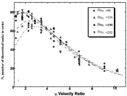
Three different models haven been used in the literature to interpret RTD data in OBRs: the tanks-in-series without interaction (compartmental model), tank-tanks-in-series with backflow, and the dispersion model. All these models are used to predict the non-ideal behaviour of the OBR on process performance. Many authors found that plug flow can be achieved with laminar flow (low net Reynolds number) and the RTD can be controlled with the oscillatory conditions independently of the net flow, as it can be observed in Figure 2.6 (Ni, 1995; Phan and Harvey, 2010; Reis et al., 2010; Stonestreet and Van Der Veeken, 1999).
The axial diffusion coefficient can be expressed via the dimensionless Péclet number, defined as:
𝑃𝑒 = 𝑢̅𝐿 𝐷𝑎𝑥
(2.8)
The Péclet number represents the ratio of the convective transport to diffusive transport, and is the reciprocal of the dimensionless axial dispersion coefficient term. It is recommended that OBRs be operated such that minimum 𝐷𝑎𝑥⁄ is acheived. According to this definition, reactors with 𝑃𝑒 > 100 𝑢̅𝐿 present an ideal plug flow behaviour, while reactors with 𝑃𝑒 < 1 present an ideal perfect mixing behaviour (Hornung and Mackley, 2009).
Figure 2.6: The dependency of the tanks-in-series model parameter, 𝑁, on the oscillatory Reynolds number for different net Reynolds (Ni et al., 2003b).
Different authors have studied the influence of the oscillatory frequency and amplitude. Palma and Giudici (2003) studied the influence of the pulsating frequency, amplitude and baffle spacing on the axial dispersion coefficient, by measurement of the RTD for a single flow phase in a pulsed sieve plate column. The results show that 𝐷𝑎𝑥 increases proportionally with an increase in the product of oscillatory
amplitude and frequency. The amplitude has a significant influence on the RTD and axial mixing compared with the frequency, and increasing amplitudes increase 𝐷𝑎𝑥 (Dickens et al., 1989; Oliva et al., 2018; Slavnić et al., 2017). This is because the amplitude directly controls the length of the eddies generated along the tube (Hamzah et al., 2012).
The multi-orifice baffle geometry has been studied and compared with the performance of single orifice baffle reactors using experimental techniques (Smith and Mackley, 2006) and numerical simulation (González-Juárez et al., 2017). From these works, it has been concluded that an increase of orifices in the baffle geometry leads to a decrease in 𝐷𝑎𝑥 (and hence an increase in the 𝑃𝑒), thereby resulting in narrow RTD curves and plug flow behaviour.
There have only been a few studies that have addressed mixing performance in OBRs in other ways than evaluating RTD. Ni et al. (1998a) characterized oscillatory baffled columns using the time necessary for a tracer to reach a specific uniform concentration into the column. Mazubert et al., (2016a, 2016b) developed characterisation methods to evaluate radial and axial fluid stretching and shear strain rate history in the OBR. The first method allows spatial mixing to be assessed and to identify the presence of chaotic flow; the second technique is useful for operations that are shear-dependent, e.g. droplet break up. McDonough et al. (2017) characterized mixing in an OBR with helical baffles using PIV and numerical simulation. They used the swirl and radial numbers to identify whether mixing is dominated by swirl or vortex flows. The swirl number describes the ratio of the axial flux of angular momentum to the axial flux of linear momentum:
𝑆𝑛 =∫ 𝑣𝑧𝑣𝜃𝑟 2d𝑟 𝑣 𝑍 𝑅 ∫ 𝑣𝑧2𝑟 d𝑟 (2.9)
where 𝑣𝑧 and 𝑣𝜃 are the axial and tangential velocity components, 𝑟 is the radial position, and 𝑅 the hydraulic radius. The radial number compares the axial flux of radial momentum to the axial flux of axial momentum: 𝑟𝑛=∫ 𝑣𝑧𝑣𝑟𝑟d𝑟 𝑣 𝑍 ∫ 𝑣𝑧2𝑟 d𝑟 (2.10)
2.I.3.2. Micromixing
Micromixing, i.e. mixing at the molecular scale, is the limiting step in the progress of instantaneous and competitive reactions. Poor micromixing can lead to a loss of conversion and the formation of undesired by-products (Baldyga and Pohorecki, 1995).
Micromixing applications, such fast precipitation and crystallization, in OBRs are a challenging area because this kind of reactor does typically not provide fast micromixing conditions, thereby leading to