Passive mitigation for magnetic between HV power line and aerial pipeline using PSO algorithms optimization

(1)

Any correspondence concerning this service should be sent

to the repository administrator:

tech-oatao@listes-diff.inp-toulouse.fr

This is an author’s version published in:

http://oatao.univ-toulouse.fr/22707

To cite this version: Djekidel, Rabah and Bessedik, Sid Ahmed

and Spitéri, Pierre and Mahi, Djillali Passive mitigation for

magnetic between HV power line and aerial pipeline using PSO

algorithms optimization. (2018) Electric Power Systems Research,

165. 18-26. ISSN 0378-7796

Official URL

DOI :

https://doi.org/10.1016/j.epsr.2018.08.014

Open Archive Toulouse Archive Ouverte

OATAO is an open access repository that collects the work of Toulouse

researchers and makes it freely available over the web where possible

(2)

Passive mitigation for magnetic coupling between HV power line and aerial

pipeline using PSO algorithms optimization

Rabah Djekidel

a,⁎

, Sid Ahmed Bessedik

a

, Pierre Spiteri

b

, Djillali Mahi

a

a_{Department of Electrical Engineering, LACOSER laboratory, University Amar Telidji, Laghouat, 03000, Algeria} b_{IRIT, ENSEEIHT, BP 7122, F-31071, Toulouse Cedex, France}

Keywords: Induced voltage Faraday’s law

Particle Swarm Optimization (PSO) HV power line

Aerial pipelines Carson’s formula

A B S T R A C T

This_{paper proposes a methodology based on Faraday’s electromagnetic induction law (EMF) for evaluating the induced} voltage produced by high voltage power line on an aerial metallic pipeline located parallel in its im-mediate vicinity under normal operating condition. It also describes the procedure of the induced voltage mi-tigation using the passive loop technique combined with the particle swarm optimization algorithm (PSO). The presence of a pipeline in the vicinity of an overhead power line strongly disturbs the mapping of the magnetic induction produced by this power line. The mitigation eﬃciency is signiﬁcantly improved by optimizing the position of the loop conductors, by increasing the number of loops and the use of a shielding magnetic material of high relative permeability. The obtained simulation result is compared with that obtained by the Carson’s formulas. A good agreement was obtained.

1. Introduction

The continued increase in electricity consumption in developing regions of the world has created significant demand for energy re-sources. The development of the installations for the transport of energy sources (oil, gas) with electric power transmission networks at very high voltage levels are accelerating to satisfy electrical needs of the world’s population. These two types of transport use long distances to fulfill their functions. Thus, the sharing of a common right-of-way be-tween the two transporters operating along their routes is inevitable. In fact, the overhead AC high voltage power transmission lines (HVTLs) generate high levels of extremely low frequency electric and magnetic fields. These generated fields can induce currents inside the human body and metallic objects located in the vicinity of these HV trans-mission lines. Therefore, it is necessary to assess and analyze the in-terference levels between these transmission lines and the metallic pi-pelines placed inside the right-of-way.

Generally there are three coupling modes of interference to be considered, the capacitive coupling; inductive coupling and conductive coupling, which produce an induced voltage in the metallic pipelines, the inductive eﬀect is the most important from among those three couplings[1–3].

In the last years, several important studies on electromagnetic in-terferences have been conducted [4–14], based on the

recommendations reported by these research studies, a number of re-ports, standards and guides have been established, to deﬁne the safety limits values of voltages and currents under normal operating condi-tions and fault condicondi-tions[15–19].

In this study, the magnetic coupling (inductive coupling) between the HV power lines and aerial metallic pipelines under normal network operating conditions is processed by means of a quasi-static numerical modeling. The purpose of this paper is to quantify the safety aspects of the operator and the personnel coming into contact with the pipeline, as well as an optimum location for the passive mitigation has been sug-gested where the induced voltage safety limits recommended by the standards[15–17]are exceeded. Also, an appropriate location for the pipeline which gives a better reduction of the induced voltage on the pipeline can be chosen using the Particle Swarm Optimization (PSO) algorithm.

In recent years, Particle Swarm Optimization (PSO) has been suc-cessfully and widely applied in various areas of electric power and high voltage engineering. PSO is a stochastic population based optimization approach that may be used to ﬁnd optimal solutions to numerical and qualitative problems. This technique was developed by Kennedy and Eberhart in 1995 and is inspired by the social behavior of insects and animals searching for food[20–22].

The present paper is structured as follows. Section2gives a brief presentation of the magnetic coupling between the AC transmission

⁎_{Corresponding} author.

E-mail address: r.djekidel@lagh-univ.dz (R. Djekidel). https://doi.org/10.1016/j.epsr.2018.08.014

(3)

lines and the aerial parallel pipeline. The calculation methods used for the evaluation of magnetic coupling and optimized mitigation are presented in Sections3and4. Finally, Section5describes the Carson’s method that validated the simulation results.

2. Magnetic coupling from power lines to pipelines

The magnetic coupling is the result of the magnetic ﬁeld generated by the power lines, as shown inFig. 1. Aerial and underground pipe-lines running parallel to/or in close proximity to transmission pipe-lines are subjected to induced voltages by the time varying magnetic ﬁelds produced by the transmission line currents. The induced electromotive force causes currents circulation in the pipeline and voltages between the pipeline and the surrounding earth[16,19,23].

3. Magnetic coupling evaluation

3.1. Magnetic ﬂux density calculation

The intensity of the magnetic induction⎯→B⎯ due to the currents Ii

flowing in supposed infinitely long horizontal conductors is obtained by the direct application of the Ampere’s law and superposition principle of the partial results. The image theory of the conductors can be applied taking into account the penetration depth De; indeed, the images of the conductors are located at a depth in the ground, much greater than the height of the conductors above ground. The effect of currents induced in the de-energized conductors (earth wires and pipeline) must also be taken into account in this calculation.

In this analysis of magnetic coupling and mitigation between the high-voltage power line and the aerial pipeline, the following simpli-fying assumptions were applied[24]:

– The conductors are horizontals and parallel to a ﬂat ground on an inﬁnite distance;

– The average height of the conductor is taken into consideration as the tower height minus 2/3 of the sag;

– The inﬂuence of the towers and metallic objects encountered which act as screens is neglected;

– The eﬀect of varying environmental conditions on soil resistivity is neglected;

– The length of the loop is at least 15 times longer than their width. By neglecting the displacement current density in Ampere’s law, the horizontal and vertical components of the magnetic induction intensity phasors (Bhand Bv) due to all the power line conductors located at

coordinates (xi, yi) above a homogeneous earth at the desired point p

(x,y) can be calculated as follows[25–30]:

∑

= − ⎡ ⎣ ⎢ − − + +_′ ⎤ ⎦ ⎥ = ⎡ ⎣ ⎢ − − −_′ ⎤ ⎦ ⎥ = = B I y y r y y D r B I x x r x x r h µ π i n i i pi i e pi v µ π i n i i pi i pi 2. 1 2 2 2. 1 2 2 0 0 (1) where,Ii are the currents phasors ﬂowing through the conductors; μo

represents the permeability of free space; n is the total number of conductors; rpi is the distance between each conductor and desired

point p; r′piis the distance between each image conductor and desired

point p; Deis the complex penetration depth and is given by[25,26,31]:

= − = D δ e δ ρ f 2 . . , 503 e jπ4 s (2) where, δ is the skin depth of the ground; ρsis the earth resistivity

ex-pressed as (Ω m); f is the frequency of the current in (Hz); j is the imaginary number.

The rms value of resultant magnetic induction at the desired point p can be calculated as:

= +

Bt Bh2 Bv2 (3)

The induced currents circulating in the de-energized conductors (earth wire and pipeline) can be found by solving the following equa-tion using the Gauss method[32,33]:

= − −

I Z Z I

[ ]g [ g1].[ gc].[ ]c (4) where, Zgc is the matrix of mutual impedances between the

de-en-ergized conductors and phase conductors; Zg is the self-impedances

matrix of the de-energized conductors; Ic is the matrix of currents

passing through the phase conductors.

In low frequencies, the self and mutual impedances with earth re-turn of the conductors are obtained according to Carson-Clem’s for-mulae[34,35]: ⎜ ⎟ = + + ⎡ ⎣⎢ ⎛ ⎝ ⎞⎠ ⎤ ⎦⎥⎡⎣ ⎤⎦ − − Z R π f j ω D R . .10 . .2.10 ln Ω km ii i e GM 2 4 4 (5) ⎜ ⎟ = + ⎡ ⎣ ⎢ ⎛ ⎝ ⎞ ⎠ ⎤ ⎦ ⎥⎡⎣ ⎤⎦ − − Z π f j ω D d . .10 . .2.10 ln Ω km ij e ij 2 4 4 (6) where, Riis the DC resistance per unit length of conductor in (Ω/km),

RGMis the geometric mean radius of the conductor in (m); dijis the

distance between the conductor i and the conductor j.

These Carson-Clem’s simpliﬁed expressions are generally suﬃ-ciently accurate when the mutual distance dijbetween conductors i and

j is less than 15% of the equivalent earth return distance De[35].

3.2. Induced voltage calculation using Faraday’s law of induction

The basic principle of the induced voltage due to high voltage power lines on a nearby conductor or a pipeline, which forms a closed loop, is the Faraday’s law of induction. This law explains that a variable mag-netic field over time can induce an electromotive force on the pipeline. The total magnetic flux due to the sinusoidal variation of all currents flowing in conductors of the overhead power line through the pipeline can be calculated from the formula given below[25,27,36,37].

∫

= ⎯→⎯ → ϕ_p Lp B d r. r r h 1 2 (7) where, Lp is the length of pipeline, Bhis the magnetic induction

com-ponent perpendicular to the plane that contains the pipeline conductor. Generally the pipeline is represented as a long lossy transmission conductor, with a return path through the earth, which constitutes a loop located at the coordinates (xp1, yp1) and (xp2, yp2), as shown in

Fig. 2, applying the coordinates of the line conductors and the pipeline [25,27,36,37].

(4)

∑

= − − + + + − + − = ϕ µ L π I x x y D y x x y y . 4. ln ( ) ( ) ( ) ( ) p p i n i p i p e i p i p i 0 1 2 2 2 2 1 2 1 2 (8)

Using the calculated total magnetic ﬂux and applying Faraday’s law, the induced voltage on the pipeline can be found using the following expression[25,27,36,37]:

= −

Vp j ω ϕ. . p (9)

where, ω is the angular frequency in (rad/s).

The minus sign indicates that the induced voltage will oppose the change in magnetic ﬂux.

This induced voltage on the pipeline can also be represented using phasors (complex numbers).

=

₍

− ∘

₎

V ep. j θ ω ϕ e. .p j θ

._Vp . ϕp 90

(10) where, θϕpand θVpare the phase angles of the total magnetic ﬂux and

the induced voltage, respectively.

The discharge current through a person’s body that touches acci-dentally the pipeline can be computed using Thevenin’s theorem, it is limited by the combination of the body resistance, the ground re-sistance to earth and the pipeline’s impedance. The expression of the discharge current is given by[38,39]:

= + + = I V Z R R V Z s p p b c p t (11)

where, Rbis the body resistance in (Ω); Rcis the ground resistance in

(Ω) and Zp is the impedance of the aerial pipeline with earth return in per unit length, it is calculated by the following equation[40]:

⎜ ⎟ = + + ⎡ ⎣ ⎢ ⎢ + ⎛ ⎝ ⎞ ⎠ ⎤ ⎦ ⎥ ⎥⎡⎣ ⎤⎦ − − Z ρ µ f r π f j ρ µ f r π f D r . . 3.163 .10 . . . 3.163 4. .10 . log Ω km p p p p p p p e e p 2 4 2 4 (12) where, rpis the pipeline’s radius; μpis the relative permeability of the

pipeline’s metal; ρpis the pipeline’s resistivity.

For touch voltages, for a soil with a surface resistivity, the ground resistance is calculated as[41–43]:

= × ρ

Rc 1. 5 s (13)

According to the American standard IEEE 80:2000, the overall re-sistance of the human body is usually taken equal to 1000 Ω[41–43]. The discharge current expression using phasor notation can be written as follows: = − I e V Z e . . ( ) s j θ p t j θ θ . _{I s} . Vp Zt (14) where, θIsand θZtare the phase angles of the discharge current and the

total impedance, respectively. 4. Magnetic coupling mitigation

In some cases, the induced voltage may exceed the acceptable limit recommended by the international standards. Most international reg-ulations, in Australia for example, the AS/NZS 4853: 2000 insist that security measures should be taken when the induced voltage on the pipeline exceeds 50 or 65 V under operating conditions[15–19]. On the other hand, in Europe, the CENELEC (EN 50443: 2009) imposes a stricter limit of the induced voltage on a pipeline of 60 V under steady-state conditions[19,44].

In this case, the attenuation is required to maintain the induced voltage within the permissible limit. In order to provide suitable pro-tection for people that touches or comes into contact with the pipeline section. The proposed methodology is based on the passive shielding technique in combination with the Particle Swarm Optimization (PSO) algorithm.

4.1. Installing passive shielding

Passive shielding technique of overhead power lines is achieved by the appropriate insertion of the metal auxiliary conductors connected in a loop to certain critical areas to be protected where the eﬀect of the induced voltage is very important along the section of the pipeline, by respecting the minimum distance D of safety between the conductors of diﬀerent voltages. Conducting and ferromagnetic materials can be used for low frequency AC magnetic shielding applications[45,46].

According to the Faraday’s Law of induction mentioned above in Eq. (9), an induced current flows through the closed passive loop due to time-varying currents flowing through the conductors of the power line. This current, by the Lenz’s Law, generates a magnetic induction that opposes the original induction produced by the source currents, in order to partially compensate it. The effectiveness of the passive loop compensation depends on the induced current, the loop impedance and its location[45,46].

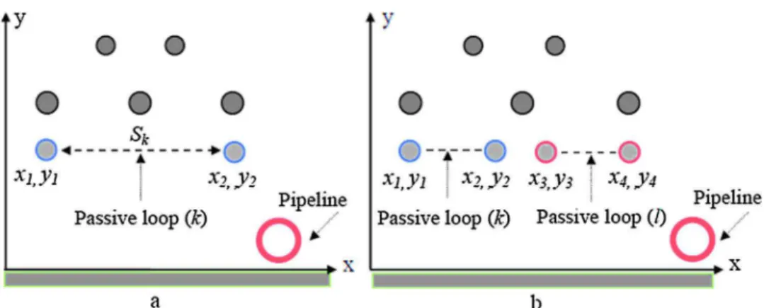
As shown in Fig. 3, the height of the closed loop's conductors is equal (y1= y2). Only the y-component of the magnetic induction

in-tensity produced by the power line is effective for magnetic flux. The magnetic flux through the passive loop caused by the sinusoidally varying currents in the power line conductors and pipeline is given by [25,27,36,37].

∑

= − − + − − + − = ϕ µ π I x x y y x x y y . ℓ. 4. ln ( ) ( ) ( ) ( ) lp i n i i i i i 0 1 2 2 2 2 1 2 1 2 (15)

where, Φlpis the magnetic ﬂux through the passive loop; ℓ is the length

of the passive loop.

Thus, according to Faraday’s law, the induced voltage on this pas-sive loop is:

= − ∘

V elp. j θ.Vlp ω ϕ. lp.ej θ.(ϕlp 90 ) (16)

The induced current ﬂowing through the passive loop is given by the following equation[25–29]:

= − I e V Z e . . ( ) lp j θ lp kk j θ θ . Ilp . Vllp Zkk (17) where the term theta (θ) indicates the phase angles of the parameters;

Zkkis the impedance per unit length of the passive loop; its value can be

easily calculated using the following equation[47]:

– For a simple loop:

(5)

= + ⎡ ⎣ ⎤⎦ Z R j ωµ µ π S r 2. . . . ln Ω m kk c r k c 0 (18) where, Rc is the resistance of the conductor constituting the passive

loop in (Ω/m); μr is the relative permeability of the conductor

con-stituting the passive loop; rc is the radius of the conductor in (m); Skis

the distance between the two parallel conductors forming the closed loop (k), this distance is calculated using the following equation (see Fig. 3):

= −

Sk x2 x1 (19)

– For a double loop: = = + = + Z Z Z R j ω Z R j ω 2. . . ln 2. . . ln kk ll kl c µ µ π d k l d k l d k l d k l lk c µ µ π d k l d k l d k l d k l . ( , ) . ( , ) ( , ) . ( , ) . ( , ) . ( , ) ( , ) . ( , ) r r 0 1 2 2 1 1 1 2 2 0 2 1 1 2 1 1 2 2 (20)

It should be noted that the inductance matrix is always symmetric, then Zkl= Zlk.

Distances separating the diﬀerent conductors of two loops (k) and (l) are calculated as follows:

= − + − = − + − = − + − = − + − d k l x x y y d k l x x y y d k l x x y y d k l x x y y ( , ) ( ) ( ) ( , ) ( ) ( ) ( , ) ( ) ( ) ( , ) ( ) ( ) 1 2 4 12 4 12 2 1 3 22 3 2 2 1 1 4 22 4 22 2 2 3 12 3 12 (21)

Finally, the resultant magnetic induction ﬁeld⎯→Br⎯ is a vector sum of the original ﬁeld created by the overhead power line and the pipeline ⎯→⎯

Bo and the compensation ﬁeld generated by the passive loop⎯→Bcomp⎯ , as shown in the equation below[25–29]:

⎯→⎯ ₌⎯→⎯ ₊⎯→⎯

Br Bo Bcomp (22)

In the same way, we can write the resultant of the induced voltage due to the overhead power line and the passive loop.

Magnetic ﬁeld compensation with the passive loop depends greatly on its location. In order to determine the optimal location of the passive loop under overhead power line, this can be achieved easily by applying optimization methods, such as the Particle Swarm Optimization (PSO).

4.2. Particle Swarm Optimization (PSO)

PSO is a robust stochastic optimization technique that may be used to ﬁnd optimal or near to optimal solutions to numerical and qualitative problems. This search optimization technique was developed by James Kennedy (social psychologist) and Russell Eberhart (electrical engineer) in 1995. It is inspired by the social behavior of swarming of insects and herding of animals when seeking food source. A brief introduction of

PSO is presented in this paper while a detailed description can be found in the references[20,22]. PSO uses a number of particles that constitute a swarm. Each particle crosses the search space looking for the global optimum[22,48]. In PSO, the velocity and position of each particle can be calculated using the following equations:

+ = + − + − t v t c rand t x t c rand t x t v ( 1) ( ) . (). (p ( ) ( )) . (). (g ( ) ( )) i i besti i besti i 1 2 (23) + = + + x ti( 1) x ti( ) v (i t 1) (24) where:

xiand viare the current position and velocity of particle at the kth

iteration of ithindividual; pbestiis the best individual particle position;

gbestiis the best swarm position; function rand () is a random number

between (0,1); constant c1, c2are learning factors, usually c1= c2= 2.

The objective in this application is to adapt Particle Swarm Optimization algorithm (PSO) to Faraday’s Law. The PSO algorithm description of the procedure can be written as follows[49,50].

Step 1: Initialize a population of particles with random positions and velocities in the problem search space;

Step 2: Evaluate the ﬁtness of each particle according to the ob-jective function. Current value is set as the new pbestwhen the ﬁtness

value is better than the best ﬁtness value (pbest) in history;

Step 3: Choose the particle with the best ﬁtness value of all the particles as the gbest;

Step 4: For each particle, calculate particle velocity according to Eq. (23)while update particle position according to Eq.(24);

Step 5: Go to step2, and repeat the process until stopping criteria are satisﬁed.

To determine the solution which reduces the induced voltage pro-duced by the power line in the pipeline, we can use the objective function of the following form:

= − −

OF (Vind(0) Vind(res x)( ,k yk))2 (25) where, Vind(0) is the induced voltage produced by the power line on the

metallic pipeline at the given position (before shielding); Vind(res) is

the resultant induced voltage on this pipeline at the same position (after shielding).

The negative sign shows the maximization of this objective function [51].

5. Carson’s formula

The Carson’s method can be used to validate the simulation results. This technique is based on the principle of the mutual and self-im-pedances of the conductors and the metallic pipeline. The calculation of these impedances is carried out using the Carson-Clem formulas pre-viously described by Eqs.(5)and(6).

To calculate the induced voltage appearing on the pipeline due to

(6)

= − − − − −

Eind I Za. pa I Zb. pb I Zc. pc Ig₁.Zpg₁ Ig₂.Zpg₂ ₍₂₆₎

where, Ia, Ib, Ic, Ig1and Ig2are the currents ﬂowing through the phase

conductors and earth wires; Zpa, Zpb, Zpc, Zpg1 and Zpg2 are the mu-tual impedances per unit length between the power line conductors and the pipeline; a, b and c represent the phase conductors, g1, g2and p are

the two earth wires and pipeline.

Since the earth wires have zero voltage drops. Using the self and mutual impedance expressions for the earth wires conductors, the voltage drops across each earth wire circuit are given by the equations below: = + + + + ≈ = + + + + ≈ V I Z I Z I Z I Z I Z V I Z I Z I Z I Z I Z ∆ . . . 0 ∆ . . . 0 g a g a b g b c g c g g g g g g g a g a b g b c g c g g g g g g 1 1 1 1 1 1 1 2 1 2 2 2 2 2 1 2 1 2 2 2 (27)

We can deduce the induced currents in the earth wires.

= − − − = − − − + + + + + + I I I I I I I I . . . . . . g a Z Z Z b Z Z Z c Z Z Z g a Z Z Z b Z Z Z c Z Z Z g a g g g g g b g g g g g c g g g g g a g g g g g b g g g g g c g g g g 1 1 1 1 1 2 1 1 1 1 2 1 1 1 1 2 2 2 2 1 2 2 2 2 1 2 2 2 2 1 2 2 (28)

Substituting these values into Eq.(26)above, and combining terms, we obtain the equation of the induced electromotive force.

= − ′ − ′ − ′ Eind I Za. 1 I Zb. 2 I Zc. 3 (29) With, ′ = − − ′ = − − ′ = − − + + + + + + Z Z Z Z Z Z Z Z Z Z Z Z pa Z Z Z pg Z Z Z pg pb Z Z Z pg Z Z Z pg pc Z Z Z pg Z Z Z pg 1 2 3 g a g g g g g a g g g g g b g g g g g b g g g g g c g g g g g c g g g g 1 1 1 1 2 1 2 2 1 2 2 2 1 1 1 1 2 1 2 2 1 2 2 2 1 1 1 1 2 1 2 2 1 2 2 2 (30)

The induced voltage on the pipeline for a length Lpcan be found by

the following equation[2,15,16]. =

Vp Eind.Lp (31)

For this case study, we consider a 400 kV single-circuit transmission line, with two earth wires and an above ground metallic pipeline in-stalled in close vicinity[5]; the geometrical data of the overhead line circuit and pipeline are shown inFig. 4. The three-phase currents on the power line have been assumed under balanced operation with the magnitude of 1000 A, at nominal frequency f = 50 Hz. The earth is assumed to be homogeneous with a resistivity of 100 Ω m. The AC re-sistance for the phase conductor is 0.0684 Ω/km, for the earth wire is 0.0643 Ω/km and 1 Ω/km for the pipeline. The pipeline is parallel to the axis of the power line at a distance of 40 m. It has an outer radius of 0.3 m and a height above ground of 1 m. The length of parallel exposure of the pipeline and power line is 5 km. Resistivity of steel pipeline ρp= 0.17 × 10−6Ωm, relative permeability of the steel μr= 300.

6. Results and discussions

The ﬁrst step is to determine the induced currents in earth wires, as given in Eq.(4)cited above, in order to take into account the eﬀect of these currents in the magnetic induction intensity calculation,

= ∘ = − ∘

Ig1 77.4ei.(150.52)( ),A Ig2 76.9ei.( 14.16)( )A.

Fig. 5 shows the lateral distribution of the RMS magnetic flux density, at 1 m above the ground with and without the presence of an above-ground pipeline, taking into account the effect of the induced currents in the earth wires and the pipeline. Without a pipeline, it can be seen that the profile is symmetrical at the power line center, where the magnetic flux density maximum value is found at this midpoint, and then it decreases continuously as one move away from this center. On the other hand, the figure also indicates that the presence of a metal pipeline near a power line, the magnetic flux density undergoes severe distortion at the place where the pipeline is implanted.

The induced voltage due to magnetic coupling on the pipeline lo-cated at diﬀerent distances from the power line center is shown in Fig. 6. As can be seen in this ﬁgure, the induced voltage has a lower value in the power line center, then increases to some maximum value occurred at a position equal to 18 m. From this point it begins to de-crease rapidly as one move away from the power line center, in which it is becoming negligible at a position located very far from this center.

Contact tensions superior to the maximum permissible value toler-ated by the European standard 60 V may constitute a threat to the safety of the pipeline’s operating agents. Then it becomes imperative to implement protection measures to maintain the induced voltage to the recommended limit. In this case study, the pipeline is installed at a distance of 40 m from the power line center, the value of the induced

Fig. 4. 400 kV Single circuit horizontal conﬁguration line with an above-ground pipeline.

Fig. 5. Magnetic induction proﬁle at 1 m above ground with and without presence of aerial pipeline.

the magnetic field created by the power line is normally worked out in two steps: first determination of the electromotive force induced along the pipeline, then the potential difference between the pipeline and the adjacent earth [2,15,16].

It should be mentioned that this approach is mainly adapted for aerial pipelines; it is invalid for pipelines that are buried underground [15].

In case of perfect parallelism between the power line and the pi-peline, the total longitudinal electromotive force induced on the pipe-line due to the currents ﬂowing in phase conductors and earth wires can be found by the following equation [2,15,16].

(7)

voltage obtained during the simulation is 115.7 V; it is greater than the permissible limit value (safe threshold).

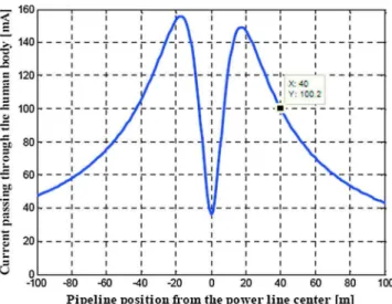
The variation of the current ﬂowing in a person’s body coming into contact with the pipeline as a function of the pipeline location is illu-strated inFig. 7. The shock current proﬁle obtained is similar to that of the induced voltage; this current is proportional to the touch voltage on the aerial pipeline. The higher the touch voltage, the higher is the shock current. In this case study, the current passing through the man for accidental contact with the pipeline is 100.2 mA. This level of current is very high and the person cannot survive this electric shock. Therefore, from a personnel safety viewpoint, it is necessary to protect against this hazard by implementing an appropriate mitigation technique.

The used mitigation system consists to install a single or double loop between the lowest phase and the ground of conductive or ferromag-netic material. The loop’s location must be optimized to ensure a good eﬃciency of electromagnetic shielding.

The variation of objective function that is used to evaluate the op-timal location of loops with number of generations is given inFig. 8. The change in value of this function illustrates the searching and op-timization processes undertaken by the PSO algorithm. The objective is to maximize this function given by Eq.(25), as illustrated in this ﬁgure. The evolution of the algorithm is increased in order to determine the smallest value of the induced voltage on the pipeline according to the search area.

The simulation results for the shielding loops position are presented

inFigs. 9 and 10, where it becomes obvious that the search algorithm converge quickly to these optimum values.

For a variable location of a pipeline along the power line corridor,

Fig. 6. Induced voltage proﬁle on the aerial pipeline.

Fig. 7. Intensity of shock current ﬂowing through the human body.

Fig. 8. Objective function variation with number of iterations.

Fig. 9. Optimum position of the conductors of the single passive loop.

(8)

the magnetic induction profile without and with passive shielding loop in conductive material is presented inFig. 11. It can be seen that the initial maximum magnetic induction is less intense at the power line center and increases to a maximum value at a location about 11 m and then gradually decreases as we get further away from this center. After optimizing the coordinates of passive loop for magnetic induction mi-tigation, on the same figure, we see a significant reduction in the peak value of the magnetic induction inside the passive loop and its im-mediate vicinity.

With the double passive loop as shown inFig. 12, the use of double loop ensures eﬀective and suitable reduction in the values of the magnetic induction along the power line corridor.

Fig. 13shows the shapes of the polarization ellipses described by the magnetic induction vector as a function of its vertical and horizontal components at the pipeline’s location (y = 40 m, z = 1 m). It is clear that the ellipses do not rest in the same plane; the ellipse described by the vector of the original magnetic induction is ahead of the ellipses of the resulting magnetic induction with passive shielding with a decrease in the values of the vertical and horizontal components. As a result, the resulting magnetic induction is generally reduced thanks to the

opti-mized coordinates of the passive magnetic shielding. _{Induced voltage on the aerial pipeline by changing the pipeline’s} location before and after the installation of passive shielding in con-ductive material is shown inFig. 14. After applying the optimization method, as can be seen in thisﬁgure that the induced voltage is very small at power line center, then increases until it reaches a maximum. After this pipeline location, the induced voltage decreases continuously with increasing the pipeline's location where it becomes almost negli-gible far from the power line center.

It is important to note that a considerable reduction in the values of the induced voltage is observed, with a simple loop, in a limited interval of pipeline location. The values of these voltages slightly exceed the limits allowed by the European standard, while with a double loop,and along the pipeline location interval, all calculated values of these vol-tages are below the threshold limit.

Induced voltage on the aerial pipeline as a function of its location without and with passive shielding in ferromagnetic material having a relative permeability μr= 5 is presented inFig. 15. It is obvious that a

very signiﬁcant reduction in the induced voltage can be eﬀected; no-tably in the interior region of the loop shield. Consequently, the use of a magnetic material with a relative permeability μr much greater than 1 produces good shielding.

Accordingly, in our case study, when a shielding loop is installed above the ground, the induced voltage on the pipe is reduced; the

Fig. 11. Magnetic induction proﬁle at 1 m above ground without and with simple passive loop.

Fig. 12. Magnetic induction proﬁle at 1 m above ground without and with double passive loops.

Fig. 13. Polarization ellipses described by the magnetic induction vector at pipeline’s location without and with the loops shielding.

Fig. 14. Induced voltage proﬁle on the aerial pipeline without and with passive shielding (conductive material μr= 1).

(9)

values obtained are shown inTable 1.

The eﬀectiveness of the loop shielding is generally assessed as the ratio between the initial induced voltage, divided by the resulting in-duced voltage with the passive loop mitigation along the pipeline’s position. The result is illustrated inFig. 16. In this case study, the pi-peline is laid at a location of 40 m from the mid point of the right of way. For a conductive material constituting the passive loop, the simple passive loop reduces a maximum the induced voltage of its initial value with a ratio of 1.4, while the maximum induced voltage reduction for double passive loop is 1.56.

For a ferromagnetic material (ur= 5), the simple passive loop

provides a reduction factor equal to 1.8. On the other hand, the double passive loop causes an important factor, which is equal to 2.41.

The peak of the induced voltage reduction factor observed in the

same ﬁgure is located at a lateral position of the pipeline of 13 m for the double passive loop. As a result, it is suggested that the pipeline be located at this position so that the induced voltage on the pipeline is very reduced.

Fig. 17shows the variation of the induced voltage reduction factor on the pipeline at lateral position of 40 m, as a function of the diﬀerent values of relative permeability of the passive loop conductor. The ap-pearance of this ﬁgure shows a non-linearity, there is a rapid evolution in reduction factor for values of relative permeability less than 50. From this value the increase in the factor becomes slower.

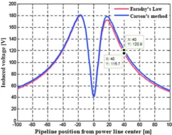
To validate the simulation results obtained with the proposed method, the induced voltage can be calculated using the Carson's method. A comparison between these two approaches is made and the results are presented inFig. 18, the analysis of the graphs of this ﬁgure shows a perfect agreement between the simulation results with a maximum relative error which does not exceed 5%. This comparison makes it possible to conﬁrm the results obtained. Furthermore, it va-lidates the adopted method.

7. Conclusion

This paper presents a rigorous quasi-static modeling to evaluate the magnetic coupling and its mitigation between an overhead power line 400 kV and aerial metallic pipeline located near this power line. From

Fig. 15. Induced voltage proﬁle on the aerial pipeline without and with passive shielding (ferromagnetic material μr= 5).

Table 1

Induced voltage on pipeline before and after applying the mitigation operation.

Relative permeability of conductor loop Without passive loop With passive simple loop With double passive loop Conductive shielding μr= 1 115.7 V 84.46 V 74.24 V Ferromagnetic shielding μr= 5 64.26 V 48.1 V

Fig. 16. Passive shield reduction factor.

Fig. 17. Reduction factor variation as a function of the relative permeability of the passive loop conductor.

(10)

network and a neighboring pipeline, Proceedings of the 62nd Annual Meeting of the American Power Conference, Chicago (April), 2000, pp. 311–316.

[2] M. Nassereddine, J. Rizk, A. Hellany, M.H. Nagrial, AC interference study on pi-peline: OHEW split factor impacts on the induced voltage, J. Electr. Eng. 14 (1)(2014) 132–138.

[3] J.R. Daconti, Electrical risks in transmission line pipeline shared rights of way, Power Technology, International Symposium on Environmental Concerns in Rights of Way, October, 2004.

[4] F.P. Dawalibi, R.D. Southey, Analysis of electrical interference from power lines to gas pipelines part I: computation methods, IEEE Trans. Power Deliv. 4 (3) (1989) 1840–1846.

[5] G. Djogo, M.M.A. Salama, Calculation of inductive coupling from power lines to multiple pipelines and buried conductors, Electr. Power Syst. Res. 41 (1) (1997) 75–84.

[6] K.A. Ellithy, A.H. AL-Badi, Determining the electromagnetic interference eﬀects on pipelines built in power transmission lines right-of-way, International Conference on Electrical Engineering (2002) 1459–1464.

[7] G.C. Christoforidis, D.P. Labridis, P.S. Dokopoulos, Inductive interference calcula-tion on imperfect coated pipelines due to nearby faulted parallel transmission lines, Electr. Power Syst. Res. 66 (August (2)) (2003) 139–148.

[8] G.C. Christoforidis, D.P. Labridis, Inductive interference of power lines on buried irrigation pipelines, Bologna, IEEE Power Tech Conference, 1 2003, pp. 196–202.[9]

H. Goo Lee, T. Hyun Ha, Y. Cheol Ha, J. Hyo Bae, D. Kyeong Kim, Analysis of voltages induced by distribution lines on gas pipelines, Singapore, International Conference on Power System Technology, 1 2004, pp. 598–601.

[10] G.C. Christoforidis, D.P. Labridis, P.S. Dokopoulos, Inductive interference on pi-pelines buried in multilayer soil due to magnetic ﬁelds from nearby faulted power lines, IEEE Trans. Electromagn. Compat. 47 (2) (2005) 254–262.

[11] A. Hossam-Eldin, W. Mokhtar, Interference between HV transmission line and nearby pipelines, 12th International Middle-East Power System Conference (2008) 218–223.

[12] D. Stet, A. Micu, L. Ceclan, The study of the electromagnetic interferences between HV lines and metallic pipelines using a professional analysis software, 2nd International Conference on Modern Power Systems, Romania (November), 2008. [13] D. Micu, L. Czumbil, A. Ceclan, L. Darabant, D. Stet, G.C. Christoforidis,

Electromagnetic interferences between HV power lines and metallic pipelines evaluated with neural network technique, 10th International Conference on Electrical Power Quality and Utilisation, IEEE, Poland, 2009.

[14] D.D. Micu, G.C. Christoforidis, L. Czumbil, AC interference on pipelines due to double circuit power lines: a detailed study, Electr. Power Syst. Res. 103 (2013) 1–8.

[15] Australian New Zealand Standard, Electrical Hazards on Metallic Pipelines, Standards Australia, Standards New Zealand, (AS/NZS- 4853), (2000). [16] CIGRE, Guide Concerning Inﬂuence of High Voltage AC Power Systems on metallic

Pipelines, Working group (36.02) (1995).

[17] NACE Standard, Mitigation of Alternating Current and Lightning Eﬀects on Metallic Structures and Corrosion Control Systems, (SP0177), (2014).

[18] CSA Standard, Principles and Practices of Electrical Coordination Between Pipelines and Electric Supply Lines, Canadian Standards Association (C22–3) (6) (January 2013).

[19] EN 50443, Eﬀects of electromagnetic interference on pipelines caused by high

voltage A.C. railway systems and/or high voltage A.C, Power Supply Systems, CENELEC Report (No: ICS 33.040.20; 33.100.01) (2009).

[20] J. Robinson, R. Yahya, Particle swarm optimization in electromagnetic, IEEE Trans. Antennas Propag. 52 (February) (2004) 397–407.

[21] M.S.H. Al-Salameh, M.A.S. Hassouna, Arranging overhead power transmission line conductors using swarm intelligence technique to minimize electromagnetic ﬁelds, Prog. Electromagn. Res. B 26 (2010) 213–236.

[22] S.A. Bessedik, H. Hadi, Prediction of ﬂashover voltage of insulators using least squares support vector machine with particle swarm optimization, Electr. Power Syst. Res. 104 (November) (2013) 87–92.

[23] R. Djekidel, D. Mahi, Calculation and analysis of inductive coupling eﬀects for HV transmission lines on aerial pipelines, Przegląd Elektrotechniczny R. 90 (9) (2014) 151–156.

[24] P. Cruz, C. Izquierdo, M. Burgos, Optimum passive shields for mitigation of power lines magnetic ﬁelds, IEEE Trans. Power Deliv. 18 (October (4)) (2003) 1357–1362.[25] K. Yamazaki, T. Kawamoto, Hi. Fujinami, Requirements power line magnetic ﬁeld mitigation using a passive loop conductor, IEEE Trans. Power Deliv. 15 (April (2)) (2000) 646–651.

[26] A.R. Memari, W. Janischewskyj, Mitigation of magnetic ﬁeld near power lines, IEEE Trans. Power Deliv. 11 (July (3)) (1996) 1577–1586.

[27] R. Mardiana, M. Poshtan, Mitigation of magnetic ﬁelds near transmission lines using a passive loop conductor, IEEE. Conference and Exhibition (GCC) (2011) 665–668.

[28] R. Radwan, M. Abdel-Salam, A. Mahdy, M. Samy, Laboratory validation of calcu-lations of magnetic ﬁeld mitigation underneath transmission lines using passive and active shield wires, Innovative Syst. Des. Eng. 2 (4) (2011) 218–232.

[29] J.R. Riba-Ruiz, A.G. Espinosa, Magnetic ﬁeld generated by sagging conductors of overhead power lines, Comput. Appl. Eng. Educ. 19 (May (4)) (2009) 787–794. [30] CIGRE, WG 36-01, Electric and Magnetic Fields Produced by Transmission Systems.

Description of Phenomena — Practical Guide for Calculation, Publisher, CIGRE, Paris, 1980.

[31] R.G. Olsen, S.L. Backus, R.D. Stearns, Development and validation of software for predicting ELF magnetic ﬁelds near power lines, IEEE Trans. Power Deliv. 10 (July (3)) (1995) 1525–1534.

[32] A. Taﬂove, J. Dabkowski, Mutual Design Considerations for Overhead Ac Transmission Lines and Gas Transmission Pipelines, Final Report. EPRI, Electric Power Research Institute. Engineering Analysis 1 (EL-904) (September 1978).[33] Transmission Line Reference Book. 345 kV and Above (UHV), Electric Power Research Institute, General Electric Company, 1982.

[34] K. Sunderland, M. Coppo, M. Conlon, R. Turri, A correction current injection method for power ﬂow analysis of unbalanced multiple-grounded 4-wire distribu-tion networks, Electr. Power Syst. Res. 132 (2016) 30–38.

[35] M. Albano, R. Turri, S. Dessanti, A. Haddad, H. Griﬃths, B. Howat, Computation of the electromagnetic coupling of parallel untransposed power lines, IEEE. Power Engineering Conference 1 (2006) 303–307.

[36] P.C. Romero, J.R. Santos, J.C. del-Pino-López, A. de-la. Villa-Jaén, J.L.M. Ramos, A comparative analysis of passive loop-based magnetic ﬁeld mitigation of overhead lines, IEEE Trans. Power Deliv. 22 (July (3)) (2007) 1773–1781.

[37] B.Y. Lee, S.H. Myung, Y.G. Cho, et al., Power frequency magnetic ﬁeld reduction method for residents in the vicinity of overhead transmission lines using passive loop, J. Electr. Eng. Technol. 6 (November (6)) (2011) 829–835.

[38] M.A. El-Sharkawi, Electric Safety: Practice and Standards, CRC Press, 2014. [39] IEEE Std 524-2003, Guide to the Installation of Overhead Transmission Line

Conductors, National Electrical Safety Code. IEEE. The Institute of Electrical and Electronics Engineers (2004).

[40] Nasser D. Tleis, Power Systems Modeling and Fault Analysis. Theory and Practice, Elsevier, 2008.

[41] Guide to Power System Earthing Practice: New Zealand Electricity Networks, Electricity Engineers’ Association, 2009.

[42] IEEE Std 80-2013, Guide for Safety in AC Substation Grounding. IEEE (2013).[43] Technical speciﬁcation, basic safety publication: Eﬀects of current on human beings

and livestock, IEC (TS 60479-1) (2005).

[44] CEFRACOR, Recommendations for the Compatibility of Grounding and Cathodic Protection, Committee for Cathodic Protection and Associated. PCRA 004 (October 2005).

[45] CIGRE WG. C4.204, Mitigation Techniques of Power Frequency Magnetic Fields originated from Electric Power Systems, CIGRE. Technical Brochure (373)(February 2009).

[46] A.K. Deb, Power line Ampacity System. Theory Modeling and Applications, CRC Press, 2000.

[47] M. Książkiewicz, Passive loop coordinates optimization for mitigation of magnetic ﬁeld value in the proximity of a power line, Comput. Appl. Electr. Eng. 13 (2015) 77–87.

[48] P. Smita, B.N. Vaidya, Optimal power ﬂow by particle swarm optimization for re-active loss minimization, Int. J. Sci. Technol. Res. 1 (February (1)) (2012) 1–6. [49] W.F. Abd-El-Waheda, A.A. Mousab, M.A. El-Shorbagyb, Integrating particle swarm

optimization with genetic algorithms for solving nonlinear optimization problems, J. Comput. Appl. Math. Elsevier 235 (January (5)) (2011) 1446–1453. [50] M.G. Masooleh, S. Ali, S. Moosavi, An improved fuzzy algorithm for image

seg-mentation, World Acad. Sci. Eng. Technol. 38 (2008) 400–404. [51] J. Burke, Math 407A: Linear Optimization, Lecture 4: LP Standard, Math Dept.

University of Washington (January 2010). these results it is evident that the presence of metallic pipeline disturbs

the magnetic induction distribution at pipeline location due to induced current which it generates.

The induced voltage on the pipeline located at diﬀerent distances from the power line center is presented. The induced voltage is less intense at the center, as the position of the pipeline is moved away from this center. The induced voltage increases to reach a maximum value, and then gradually reduces where it becomes very neglected far from the center of the power line. The shock current proﬁle passing through the body of a person that touches the pipeline has a behavior similar to that observed for the induced voltage; the level obtained is high enough to cause damage.

The passive mitigation loop technique using conductive and ferro-magnetic material with a Particle Swarm Optimization (PSO) algorithm is applied; the proposed mitigation eﬀectively reduces the induced voltage on the pipeline. The shielding performance can be greatly in-creased by using a ferromagnetic material with high relative perme-ability. The result of the numerical simulation is compared to result obtained by Carson’s formulas. The comparison shows that a good correlation is reached which conﬁrms the validity of the proposed method.

References