Dionne : HEC Montréal and CIRPÉE Gauthier : HEC Montréal
Hammami : Caisse de Dépôt et Placement du Québec Maurice : Caisse de Dépôt et Placement du Québec
Simonato : Corresponding author. HEC Montréal and CIRPÉE jean-guy.simonato@hec.ca ; Phone: 514 340-6807
The authors acknowledge the financial support from the National Science and Engineering Research Council of Canada (NSERC), the Fonds québécois de recherche sur la nature et les technologies (FQRNT), the Social Sciences and Humanities Research Council of Canada (SSHRC), the Center for research on E-finance (CREF), the Canada Research Chair in Risk Management, and the Institut de Finance Mathématique de Montréal. Preliminary versions were presented at the 2006 North American Winter Meeting of the Econometric Society, the 2006 European Finance Association conference, the 18th Annual Derivatives Securities and Risk Management Conference and the 2010
Cahier de recherche/Working Paper 10-42
A Reduced Form Model of Default Spreads with Markov-Switching
Macroeconomic Factors
Georges Dionne
Geneviève Gauthier
Khemais Hammami
Mathieu Maurice
Jean-Guy Simonato
Novembre/November 2010
Abstract:
An important research area of the corporate yield spread literature seeks to measure the
proportion of the spread that can be explained by factors such as the possibility of
default, liquidity, tax differentials and market risk. We contribute to this literature by
assessing the ability of observed macroeconomic factors and the possibility of changes
in regime to explain the proportion of yield spreads caused by the risk of default in the
context of a reduced form model. For this purpose, we extend the Markov Switching
risk-free term structure model of Bansal and Zhou (2002) to the corporate bond setting and
develop recursive formulas for default probabilities, risk-free and risky zero-coupon bond
yields as well as credit default swap premia. The model is calibrated with consumption,
inflation, risk-free yields and default data for Aa, A and Baa bonds from the 1987-2008
period. We find that our macroeconomic factors are linked with two out of three sharp
increases in the spreads during this sample period, indicating that the variations can be
related to macroeconomic undiversifiable risk. The estimated default spreads can
explain almost half of the 10 years to maturity industrial Baa zero-coupon yields in some
regime. Much smaller proportions are found for Aa and A bonds with numbers around
10%. The proportions of default estimated with credit default swaps are higher, in many
cases doubling those found with corporate yield spreads.
Keywords: Credit spread, default spread, Markov switching, macroeconomic factors,
reduced form model of default, random subjective discount factor, credit default swap,
CDS
1
Introduction
Several empirical studies have recently been performed on corporate yield spreads, measured as the difference between the corporate and treasury yield to maturity. These studies attempt to explain some of the observed features of corporate spreads through time. In this article we synthesize two research directions recently explored by this literature. We investigate whether a reduced form model with observed macroeconomic risk factors following a Markov-switching process can help explain the spread behavior through time. The model and the empirical study proposed here can also be seen as an extension of the Elton et al. (2001) model to a risk averse setting. In Elton et al. (2001), an assumption of risk neutrality was needed to justify the use of observed default probabilities in a bond pricing model specified under the risk neutral measure. Although risk premia were estimated empirically with Fama-French factors, risk aversion was not explicitly incorporated in their theoretical modeling approach. The model developed here is entirely specified under the objective measure in a risk averse setting, avoiding the need for a risk neutrality assumption.
The motivation for examining macroeconomic fundamentals as drivers of the spread behavior comes from the link between interest rates and output from firms and the macroeconomy. These variables, which should influence yield spreads, fluctuate over the business cycle. It should thus be anticipated that macroeconomic fundamentals play a role in explaining the spread behavior through time. Recently, some attempts have been made to associate macroeconomic activity to the spreads in the context of structural models. For example, Pesaran et al. (2006) examine an econometric model linking credit risk and macroeconomic variables in a Merton-type structural model. Chen et al. (2009) explore how a structural model using pricing kernels that are successful in solving the equity premium puzzle performs in explaining the spread. David (2008) looks at how investors’ learning from inflation helps to generate realistic credit spread levels. With the exception of Amato and Luisi (2006), where a model of credit spread with both latent and observed macro variables is examined, little research has been done in the context of reduced form models. Further work on the reduced form type models and the macroeconomy is thus an interesting addition to the literature because these models often require fewer inputs in the calibration stage.
The motivation for examining the influence of macroeconomic variables in such a framework comes from empirical evidence suggesting that switching regimes are better descriptions of these variables and risk-free interest behavior than single regime models. See for example Evans (2003), Ang, Bekeart and Wei (2008), Bansal and Zhou (2002) and Dai, Singleton and Yang (2007). Because the possibility of changes in regime might influence macroeconomic factors and risk-free interest rates, it is only natural to assume that this might also affect corporate yield spreads. Davies (2008) finds that this is indeed the case and that a Markov-switching model summarizes some properties of spread times series well. Cenesizoglu and Essid (2010) also provide evidences of switching behavior while examining the effect of monetary policy on credit spreads.
To introduce macroeconomic factors and the possibility of changes in regime in a reduced form spread model, we extend the switching regime risk-free term structure model of Bansal and Zhou (2002) to the risky corporate setting. Starting from the first order condition of the intertemporal consumption problem with a power utility function and a random subjective discount factor, we assume that consumption and inflation dynamics are governed by two independent Markov chains. Using a log linear approximation we derive closed form recursive formulas for risk-free and risky bond yields, default probabilities, and credit default swap premia, which are all functions of the growth rates of our two observed factors. We also consider recovery rates varying with the states of consumption growth. We then measure the default spread generated by this approach by calibrating the model with financial data.
Our calibration approach proceeds without yield spread data. Corporate yield spread levels might be influenced by several factors such as the possibility of default, liquidity, market risk or taxes. Because our goal is to measure the proportion of the spread brought by the possibility of default, our model accounts for this dimension only, avoiding the potential misspecifications of other factors. Thus, fitting the model developed here with spread data could produce biased results because of the omitted factors. We therefore rely on an indirect strategy that uses aggregate consumption growth, inflation, risk-free yield curves and default data to obtain the parameter values required to measure the proportion of the yield spreads which can be explained by the possibility of default alone.
parameters with aggregate consumption and inflation data. Using the parameters obtained in the first step, we then extract utility parameters from the term structure of risk-free rates. In a third step, with the parameter values obtained in the preceding steps, we calibrate the parameters linking our theoretical default probabilities with the macroeconomic risk factors to match the observed default probabilities obtained from default data. The default yield spreads implied by our model can then be computed and analyzed with an assumed structure for the recovery rates.
Our results show that the default spread exhibit different sensitivities to consumption and inflation depending on the possible regimes. We find that the model can reproduce some key properties of observed spreads, such as the sharp increases observed in two out of three recessions present in our sample period. These two sharp increases are associated with a low consumption growth and high inflation uncertainty regime identified by our Markov-switching process. This result is interesting because it indicates that, in some regime, the spread level is sensitive to a macroeconomic market wide undiversifiable risk. Such a result is supported by recent studies such as Farnsworth and Li (2007), who provide evidence of systematic factors associated with default risk. Our results also indicate that sharp increases in spreads are not necessarily linked to macroeconomic variables. For example, the sharp increase in 2001 is not captured by our model because this period is found to be in a high consumption growth and low inflation risk regime. This result is in line with the literature on forecasting models where the consumption indicator of economic activity was found to be a poor predictor of the 2001 recession (Evans et al 2002; Stock and Watson, 2003). We also find that risk aversion does not greatly influence the proportion of the spread caused by the risk of default. This result can, in part, be attributed to the low volatility of consumption growth and inflation during the studied period which are used as the sole factors in the model. We obtain estimates of default spread proportions varying through the different regimes. For example, these proportions for 10 years to maturity Baa yields range from 28% to 43%, while they are around 10% for Aa and A yields. (Table 7). The proportions of default are also estimated with credit default swaps, which are instruments less influenced by liquidity or tax considerations. With these, much higher proportions are found with numbers around 21%, 35% and 76% for Aa, A and Baa.
Section 2 presents our theoretical models and formulas for the risk-free zero-coupon bonds, the risky zero-coupon bonds and the default probabilities. Section 3 presents our estimation results
and calibration procedures. Section 3.7 analyzes the estimated default spreads for industrial Aa, A and Baa bonds. Section 4 extends the analysis to credit default swaps. Section 5 concludes the paper.
2
Model
The model developed here starts from the well known first-order condition of the intertemporal consumption problem as described in, for example, Cochrane (2005). Because we attempt to model nominal bond prices, we account for the future growth rates of the price level and real consumption. We assume that the future evolution of these variables is well described by a Markov-switching process.
Let Ct denote the real personal consumption expenditures per capita at time t, and Πt the
ratio of nominal over real consumptions (consumption price index) at time t with t ∈ N . Here, the time variable is expressed in quarters and the continuously compounded quarterly growth rates are defined as ct = ln Ct− ln Ct−1 and πt = ln Πt− ln Πt−1. We assume that ct and πt follow an
autoregressive model with switching regimes ct= acsc t + b c sc tct−1+ e c t (1a) πt= aπsπ t + b π sπ tπt−1+ e π t (1b)
where sct ∈ {1, 2} is the state of consumption at time t and sπt ∈ {1, 2} is the state of inflation at time t. The error terms ect and eπt are i.i.d. Normal noises with zero mean, standard deviations σscc t and σ π sπ t and covariance ρstσ c sc tσ π sπ t with st ={s c t, sπt} i.e. st ∈ {(1, 1) , (1, 2) , (2, 1) , (2, 2)} . The
states of consumption growth and inflation are assumed to follow two independent Markov chains with transition matrices
ϕc = ( ϕc11 1− ϕc11 1− ϕc22 ϕc22 ) , ϕπ = ( ϕπ11 1− ϕπ11 1− ϕπ22 ϕπ22 ) . These Markov chains are also assumed to be independent of past values of c and π.
Define the σ−field Gt= σ (Cu, Πu, su : u∈ {0, 1, ..., t}) . It may be interpreted as the information
available at time t if one observes the evolution of consumption growth, inflation, and the state of consumption and inflation up to time t.
To obtain our pricing equations, we assume a standard time-separable power utility function for the investor with a subjective discount factor coefficient which depends on the future states of the Markov chain. We are thus allowing the subjective discount factor parameter to be different in the different possible regimes1. As discussed in Cochrane (2005), the standard power utility framework with lognormal consumption does not easily reproduce key features of observed risk-free term structures such as a positive average slope. This parametrization for the time-preference coefficient provides an additional flexibility that will help generate average yield curves with a positive slope. Appendix A shows that, from the first order condition of the intertemporal consumption problem, the time t value of a security without default risk worth Xt+1 at time t + 1 is given by
Et [ βst+1 ( Ct+1 Ct )−γ Πt Πt+1 Xt+1 ] = Et[Mt,t+1Xt+1] (2) where Mt,t+1= exp ( ln βst+1− γct+1− πt+1 ) (3) is the nominal discount factor or the default-free pricing kernel for the time period ]t, t + 1] , βst+1 is
the subjective discount factor in state st+1 and γ the risk aversion coefficient. Et[•] is a shorthand
notation for E [• |Gt], the conditional expectation with respect to available information at time t.
Equation (2) thus proposes a pricing kernel for default-free securities which is a function of the consumption, inflation and Markov chain processes. The pricing kernel accounts for regime shift uncertainty given that parameters of the consumption and inflation at t + 1 are function of the state for the Markov chain in t + 1. As mentioned above, we also assume that this uncertainty affects the subjective discount factor β that also depends on the state of the Markov chain at t + 1.
2.1 Risk free zero-coupon bond
An exact formula for the time t value of a default-risk-free zero-coupon bond paying one dollar at time T can be obtained using the framework described above. However, such a solution is not practical. For example, with quarterly time steps, the value of a zero-coupon bond maturing in
1
Such preferences are coherent with the general framework proposed in Higashi et al. (2009). In their model, a decision maker believes that his discount factors change randomly over time according to i.i.d. shocks. Our formulation assumes a Markov chain. Apart from that, our model is consistent with their formulation. See also Salani´e and Treich (2006).
40 quarters would roughly contain 440 terms to compute. This would make the numerical imple-mentation of the exact solution unmanageable. For this reason, we instead rely on an analytical approximation developed in Bansal and Zhou (2002) for the price of a risk-free zero-coupon bond with n periods to maturity:
P (t, n, st) = exp
(
Apn,st− Bn,sp,ctct− Bn,sp,πtπt
)
(4) where st={sct, sπt} and expressions for A
p n,st, B
p,c
n,st, and B
p,π
n,st are given in Appendix B. The pricing
formula is a function of our observed factors and the states of the Markov chains. Sensitivities to the factors are given by the B functions which are determined recursively using backward induction and the terminal condition Ap0,s
T = B
p,c
0,sT = B
p,π
0,sT = 0. These expressions are functions of the
Markov-switching parameters and the actual states of consumption and inflation sct and sπt. At each point in time, four different bond prices can thus be computed because four different states are possible. Because the state of the economy is unknown at a particular point in time, we will define the theoretical zero-coupon bond price as the expected bond price, with the expectation computed over the possible states of the Markov chain whose probability can be conveniently estimated. Section 3.4 provides further details about this procedure. Factor sensitivities are also functions of the time to maturity, n = T − t, and the utility function parameters.
Although the formula in Appendix B is complex, it is possible to get some intuition by looking at the one-period case, rewritten in terms of an annualized yield to maturity:
yp(t, 1, st) = 4 2 ∑ i=1 2 ∑ j=1 ϕcsc t,iϕ π sπ t,j − ln βi,j+ γ (a c i + bcict) + ( aπj + bπjπt ) −1 2 ( σπj )2 −1 2γ2(σci) 2− γρ i,jσicσπj
where the term inside brackets is the expression for the yield to maturity, in state i, j, of a one-period risk-free bond within the power utility lognormal framework. The one-one-period bond yield in state st is the conditional expected value of the bond yields in the different possible states where
the ϕ’s are the transition probabilities. The various terms forming the bond yield in state i, j are then interpreted the usual way.
The first term of the expression within brackets is a function of the subjective discount factor. A smaller subjective discount factor (more impatient investor) is associated with higher yields because the impatient investor prefers consumption to saving. The second term, γ (aci + bcict) ,
is the risk aversion parameter multiplied by the conditional expected growth of consumption in state i, j. Given positive aci and bci, higher values of these coefficients will lead to higher expected consumption growth and higher yields. The risk aversion parameter γ > 0 makes the yield more or less sensitive to the expected consumption growth rate. The sum of the third and fourth term, (aπj + bπjπt)−12
( σjπ
)2
, is the portion of yield rewarding the investor for the expected loss in real purchasing power on the nominal one dollar bond payoff at maturity and where the variance of inflation appears because of the convexity of the bond pricing function. The fifth term, 12γ2
( σjc
)2
, is the precautionary savings effect brought by the volatility of consumption. An increase in the volatility of consumption brings more extreme low and high paths of future consumption. Because investors worry more about the low consumption states than they are pleased by the high ones, a demand for savings is created that drives down the yield on the bond. The last term, γρi,jσicσjπ,
is the inflation risk premium. A negative correlation will obtain a positive risk premia because inflation decreases the real nominal bond payoff in states where the investor needs it the most. For example, a future low consumption state would likely be associated with a high inflation path and low real value for the nominal payoff.
2.2 Risky zero-coupon bond and default spread
We consider a risky zero-coupon bond paying one dollar at T if it has not defaulted before. In case of default, the bondholder receives at the default time τ , a fraction of its market value if it had not defaulted. In this well studied context (see Duffie and Singleton 1999), the time t value of the survived risky zero-coupon bond is
e V (t, n, st) = Et [ Mt,t+1 ( 1− Lst+1ht+1) eV (t + 1, n− 1, st+1) ]
where Lst+1is the loss given default (LGD), defined as one minus the recovery rate and assumed
to depend on the states of the Markov chain. Here, ht+1 = PrGt+1[τ = t + 1| τ > t] represents
the conditional probability that the default arises within the next period of time knowing that the firm as survived at time t and having the information available at time t + 1. Because default probabilities are usually small, it is reasonable to use a first order Taylor expansion to approximate
1− Lst+1ht+1 by exp ( −Lst+1ht+1 ) . Hence e V (t, n, st) ∼= Et [ Mt,t+1exp ( −Lst+1ht+1) eV (t + 1, n− 1, st+1) ] . (5) where Mt,t+1exp ( −Lst+1ht+1 )
is our pricing kernel for the risky zero-coupon bond. We also assume that the conditional default probability ht+1is approximated by an affine function of ct+1and πt+1,
that is, ht+1∼= αst+1+ α c st+1ct+1+ α π st+1πt+1 (6) where αst+1, α c st+1 and α π
st+1 are parameters. Note that the specification (6) can produce negative
probabilities as well as probabilities larger than one. Using these assumptions and those required by the approach of Bansal and Zhou (2002), Appendix C develops the following analytical approx-imation for the prices of risky zero-coupon bonds :
V (t, n, st) = exp
(
Avn,st− Bn,sv,ctct− Bn,sv,πtπt
)
. (7)
As shown in Appendix C, the coefficients Avn,st, Bn,sv,ct and B
v,π
n,st are obtained recursively starting
with Av0,sT = B0,sv,cT = B0,sv,πT = 0. The resulting pricing formula is very similar to the risk-free case developed earlier. It is a function of the current values of our two observed factors with the loadings given by the B functions. These quantities are functions of the Markov-switching model parameters, the actual states of consumption and inflation sct and sπt, the utility function parameter values and the time to maturity. Unlike the risk-free case, however, we find the additional Li,jαi,j, Li,jαci,j and
Li,jαπi,j terms appearing because of the possibility of default.
Using the above analytical approximation and the earlier approximation for the risk-free yield, an expression for the annualized default spread, defined as the difference between the risky yield to maturity and the risk-free yield to maturity, is given by:
DS (t, n, st) = Apn,st − Avn,st + (B v,c n,st− B p,c n,st) ct+ (B v,π n,st − B p,π n,st) πt n/4 . (8)
to look at the one period case : DS (t, 1, st) = 4 2 ∑ i=1 2 ∑ j=1 ϕcsc t,iϕ π sπ t,j (9) × Li,j
αi,j+ αci,j(aci + bcict) + απi,j(aπj + bπjπt)
−1 2Li,j (( αci,jσic )2 + ( απi,jσπj )2
+ 2απi,jαci,jρi,jσicσjπ
) −απ i,j ( σπj )2 − γ(αci,j(σci)2+ ( απi,j+ αci,j ) ρi,jσicσjπ )
where the term inside brackets is the expression for the default spread, in state i, j, for a one period risky bond. The default spread in state st is the conditional expected value of the bond yield
spreads in the different possible states next period.
The first line of the term within brackets can be interpreted as one of the portions forming the expected loss next period in state i, j. In the context of a one period bond, Li,j represents the loss
given default. This quantity is multiplied by the conditional expected default probability in state i, j that is αi,j+ αci,j(aci + bcict) + απi,j(aπj + bπjπt). The signs of the αi,j, αci,j and απi,j will determine
the influence of consumption and inflation on this portion of the spread. The second and third lines are the additional impacts of potential losses brought by the convexity of our recovery factor model. Again, the sign of these terms will depend on the signs of the α’s. For example, the effect of a change in consumption volatility is not clear because it depends on the magnitude and signs of the α’s and the correlation. Hence, given ρi,j > 0 with a negative and large αci,j (relative to
the απi,j), an increase in consumption volatility will increase the spread. Finally, the risk aversion parameter interacts only with the squared volatilities and covariance of the factors. Hence, risk aversion is a second order effect whose magnitude will be determined by the relative importance of the volatilities, the covariance term, and the magnitudes and signs of the αci,j and απi,j parameters. In the context of this model, the proportion caused by risk aversion can be conveniently assessed. One can first compute the portion of the spread caused by the actuarial loss. This is the default spread with which a risk neutral investor would be satisfied. This quantity, that we label the default risk spread, can be computed by setting γ = 0 in the default spread equation i.e.
DR(t, n, st) = DS (t, n, st| γ = 0) . (10)
then be computed by difference with
DP (t, n, st) = DS (t, n, st)− DR(t, n, st). (11)
This is the spread a risk-averse investor would ask for in addition to the default risk spread. In the context of a one period bond, this quantity becomes
DP (t, 1, st) = 4× 2 ∑ i=1 2 ∑ j=1 ϕcsc t,iϕ π sπ t,j [ −γLi,j (
αci,j(σic)2+(αi,jπ + αci,j)ρi,jσciσπj
)] .
2.3 Survival probability
A final theoretical quantity obtained within the framework of this model is the term structure of survival probabilities. This quantity will be used to calibrate our model to match the default probabilities that are observed for the sample period examined in this study.
The survival probability at t, PrGt[τ > t + n | τ > t] , is the probability that the default will
occur in more than n periods from t knowing that the firm has not defaulted at time t in a given state of our macro factors at t. Because the one-period default probability is usually small, we use the approximation e−hu ∼= 1− h u to write PrGt[τ > t + n| τ > t] = Et [ t+n∏ u=t+1 (1− hu) ] as PrGt[τ > t + n| τ > t] ∼= Et [ exp ( − t+n∑ u=t+1 ( αsu+ α c sucu+ α π suπu ))]
from our assumption given in equation (6). As shown in Appendix D, an analytical approximation for this expected value is given by:
q (t, n, st) = exp ( −Aq n,st− B q,c n,stct− B q,π n,stπt ) . (12)
As in the previous cases, the coefficients Aqn,st, B
q,c
n,st and B
q,π
n,st are obtained recursively starting
with Aq0,s
T = B
q,c
0,sT = B
q,π
0,sT = 0. These coefficients are functions of the maturity n, the
Markov-switching parameters, the unobserved state st and the unknown parameters linking the one-period
3
Calibration and estimation
3.1 Empirical yield curves
To measure the capacity of our model to generate realistic default spread levels through time, estimates of the credit yield spread curves of Aa, A and Baa zero-coupon bonds are required. The spread curves are computed as the difference between the zero-coupon corporate yields and the zero-coupon risk-free yields. We explain here how these risk-free and corporate zero yields are obtained.
The risk free zero-coupon yield data comes from Gurkaynack et al. (1997) which is available from the Federal Reserve web site2. The data contains, at a daily frequency, the parameter estimates of the Svensson (1994) model from cross-sections of risk-free coupon bonds. To build our quarterly risk-free curves, we first extract the parameters at the dates that are nearest to the quarterly dates of the National Income and Product Accounts data. We then use these parameters in the Svensson (1994) model with maturities of 0.25, 0.5, 0.75, ..., 10 years to get a risk-free curve for each date of our sample.
For dates ranging from 1987-I to 1996-IV, the corporate zero-coupon yield curves are extracted from the Warga (1998) fixed income database, which contains information on monthly prices, accrued interest, coupons, ratings, callability and returns on investment-grade corporate bonds quoted at Lehman Brothers. All bonds with matrix prices and options were removed; bonds not in Lehman Brothers’ bond indexes and bonds with an odd frequency of coupon payments were also dropped. We proceed as in Dionne et al. (2010) to get the month-end estimates of the yield curves on zero-coupon bonds for each rating class from Moody’s (Aa, A and Baa). These yield curves are obtained by first estimating the parameters associated with the Nelson and Siegel (1987) model with a non-linear least-square procedure on bonds with maturities of 10 years or less3. All bonds with a pricing error higher than $5 are dropped. We then repeat this estimation and data removal procedure until all bonds with a pricing error larger than $5 were removed. Using this procedure, 776 bonds were removed (one Aa, 90 A and 695 Baa) out of a total of 33,401 bonds found in the
2
http://www.federalreserve.gov/pubs/feds/2006
3To minimize the chances of converging to a local rather than a global minimum, a grid search of 204= 160000
industrial sector. We then use these parameters in the Nelson Siegel (1987) model with maturities of 0.25, 0.5, 0.75, ..., 10 years to get a risk-free curve for each date of our sample.
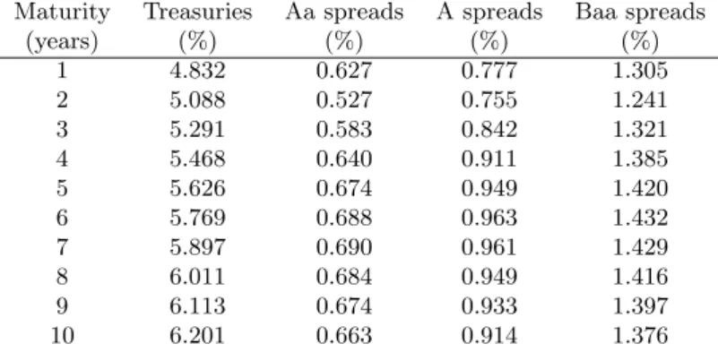
For dates between 1997-I to 2008-IV, we use the zero-coupon yield data available from Bloomberg. These yields are extracted by Bloomberg on samples of coupon bond prices with a spline approach. Bloomberg makes available maturities of 0.25, 0.5, 1, 2, 3, 4, 5, 6, 7, 8, 9, 10, 15, 20 and 30 years on bonds from the industrial sector rated (Standard and Poor’s) AA, A+, A, A-, BBB+, BBB, BBB- on a daily frequency. We first extract the data for the dates that are the nearest to the quarterly dates of the National Income and Product Account data. For this sample, for each date and maturity, we first aggregate the yields of A rated bonds with an average i.e. the yield of an A rated bond is the average yield from A+, A, and A- rated bonds. The same is done for BBB bonds. Because our study uses maturities 0.25, 0.5, 0.75, ..., 10 years, we interpolate for these maturities using Nelson-Siegel. We thus estimate for each date, the parameters of the Nelson-Siegel model on the Bloomberg zero-coupon yields with maturities of 0.5, 1, 2, 3, 4, 5, 6, 7, 8, 9, 10 and use these parameters to compute the yields of 0.25, 0.5, 0.75, ..., 10 year bonds. Table 1 presents the average zero-coupon yield spreads for industrial Aa, A and Baa for maturities of 1 to 10 years for the 1987-2008 period.
3.2 Markov-switching parameters
This section describes how the parameters of the Markov-switching model are estimated. Let θ denote the set of parameters associated with the growth rate equations that is θ = (ac1, ac2, bc1, bc2, aπ1, aπ2, bπ1, bπ2, σ1c, σ2c, σ1π, σπ2, ρ1,1, ρ1,2, ρ2,1, ρ2,2) and the transition probability parameters
ϕ = (ϕc11, ϕc22, ϕ11π , ϕπ22). From the time series of consumption levels C0, ..., CT and price index
levels Π0, ..., ΠT from which we create the sample c1, ...cT, π1, ..., πT, we define vt = (x1, ..., xt) as
the set of observed data point up to time t and xt = (ct, πt) as the set of observed consumption
growth and inflation at t. From Hamilton (1994), the log-likelihood function based on the observed sample vT up to time T is then computed with
L (θ,ϕ; vT) =
T
∑
t=2
where
f (xt| vt−1; θ,ϕ) = ηt′× ξt|t−1
represents the conditional likelihood function of xtgiven the observed sample vt−1. The 4×1 vector
ηt contains the likelihood value of xt conditional on states i, j and the observed sample vt−1. The
4×1 vector ξt|t−1contains the probability of being in state i, j at time t conditional on the observed
sample vt−1. Appendix E describes how these quantities can be computed. The maximization of
the log-likelihood functionL (θ, ϕ; vT) is done numerically using a hill climbing algorithm.
The data series used here are the growth rate of non-durable and services personal consumption expenditures per capita (real) from the first quarter of 1957 to the last quarter of 2008 and the growth rate of the consumption price index for the same period4. The data comes from the U.S. Department of Commerce, Bureau of Economic Analysis. The data period contains nine recessions according to the NBER and many of them should be important enough to generate regime shifts. Figure 1 illustrates the temporal evolution of the two growth rates.
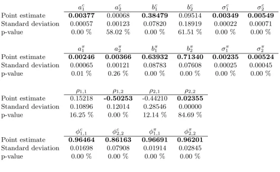
The results of the estimation procedure are presented in Table 2. For consumption, regime switching appears in the mean and the volatility. For inflation, only the volatility parameter is found to differ with the regime shifts. We also observe that ρ12 and ρ22 are statistically different
from zero.
Within the context of our regime switching model, two conditional probabilities are of interest. The ex-ante probability, ξt|t, is useful in forecasting future inflation and consumption rates based on an evolving information set. The smoothed probability, ξt|T, estimated using the entire information set available, is of interest for the determination of the prevailing regime at each time point within the sample period. To estimate ξt|T = f (st| vT; θ, ϕ) for st∈ {(1, 1) , (1, 2) , (2, 1) , (2, 2)}, we use
the following algorithm developed in Kim (1994):
ξt|T = ξt|t(×)[Φ(ξt+1|T(÷) ξt+1|t)] (14)
where (×) and (÷) means element-by-element multiplication and division respectively and where the transition matrix Φ is described in appendix E.
4
Non-durable goods and services expenditures are aggregated naively with a simple sum of both components. We have verified that this approach gives results almost identical those from the chain aggregation approach, described in, for example, Whelan (2000).
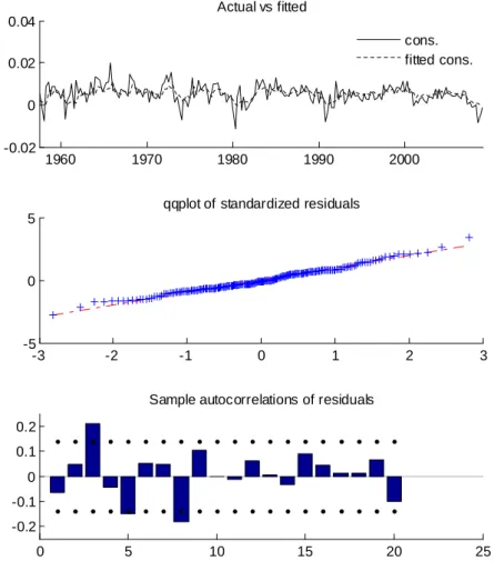
Using these probabilities, Figures 2 and 3 examine the fit of the Markov-switching model. Each figure shows three graphs. The first graph plots the actual and fitted values; the second graph shows a quantile-to-quantile plot (qqplot) of the standardized residuals; the third graph looks at the sample autocorrelation coefficients of the residuals. Because there is uncertainty about which state prevails, the fitted values are computed as the expected fitted values over the two possible states. These expected values are computed with the smoothed probabilities. The same procedure is adopted to form the residual series, which are standardized by dividing by the estimated standard deviation in each state. For the consumption growth series, the actual values are often far from the fitted ones. Despite these large residuals, the qqplot and sample autocorrelation coefficients show that the model produces nearly white noise residuals that are well described by a normal distribution. The sample autocorrelations are in most cases within the two standard deviation confidence interval around a value of zero for all lags, except for lags 3 and 8 which are slightly out. For the inflation series, the actual values are closer to the fitted one. Again, from the qqplot and sample autocorrelation coefficients, the model is shown to produce well behave Normal residuals with significant autocorrelations in lags 1, 3 and 6.
3.3 States of consumption and inflation
We examine here more closely the estimated probabilities for the state of the Markov chain for the period 1987-I- to 2008-IV which corresponds to the data period we have, regarding our risky bond information. Note that we used the estimates of θ and ϕ from Table 2.
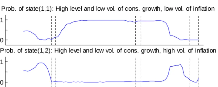
The results of the estimation procedure are presented in Figure 4. In most quarters, one of the four values of the mass function clearly dominates the other. On a total of 88 observations, 80 are larger than 0.6 and 73 are larger than 0.8. The estimated state bst at time t is the one for which
the estimated probability in vector ξt|T is the highest among all the possible states. The results are reported in Figure 5.
The interpretation of the estimated states are as follows: st = (1, 1) corresponds to a state of
high level and low consumption growth volatility combined with low volatility of inflation; st= (1, 2)
is the state of high level and low volatility of consumption growth with high volatility of inflation; st= (2, 1) corresponds to the low level and high volatility of consumption growth combined with
low volatility of inflation; finally, st = (2, 2) is for low level and high volatility of consumption
growth with more volatile inflation.
A detailed examination of the results reveals that the estimated state of consumption is 1 for two distinct time periods: 1987-I to 1990-I and for 1991-IV to 2007-I. Otherwise, the estimated state of consumption is 2. For inflation, we note two changes of regime. Indeed, the state of inflation is estimated to 2 for the time period 1987-I to 1990-IV and becomes 1 for the time period 1991-I to 2005-I and then comes back to two until the end of the sample. If we consider the system globally, the estimated state is st = (2, 2) near the 1991 and 2008 NBER recessions. In between
these NBER recessions, the system stays in state st= (1, 1), even with the presence of an official
NBER recession in 2001. Prior to the 1991 NBER recession, the estimated state is st = (1, 2).
Figure 6 illustrates the changes of regime behavior for the growth rate of our two factors. The consumption growth rate and inflation clearly exhibit different behavior in each regime.
Note that the observed average consumption growth rate and volatility are 0.51% and 0.27% during the periods corresponding to bsct = 1 while they are -0.15% and 0.37% during the periods corresponding to bsct = 2. The observed average inflation growth rate and volatility are 0.64% and 0.21% during periods for which bsπt = 1 and 0.93% and 0.59% when bsπt = 2. These numbers correspond roughly to the unconditional mean and standard deviations that can be computed from the parameter estimates. For consumption, these unconditional mean and standard deviations are 0.61% and 0.38% for bsct = 1 and 0.075% and 0.55% for bsct = 2 while they are 0.68% and 0.30% for inflation whenbsπt = 1 and 1.2% and 0.75% when bsπt = 2.
As mentioned, our model did not capture the 2001 recession for consumption growth. This conclusion seems more related to the consumption variable than the model. During the 1987-2008 period, there were three economic recessions: 06-1990/03-1991, 03-2000/11-2001, and 12-2007/06-2009. It is now known that the 2001 recession was different when compared to the other recessions. As documented by Stock and Watson (2003), the 2001 recession started when businesses cut their expenditures, particularly their investments in information technology which leaded declines in manufacturing output and stock market. During that recession, personal consumption and housing index did not register significant negative values (Evans et al., (2002)), while during the 1990 recession, consumption had a sharp fall explained by uncertainty associated with Iraq’s invasion
and the variation of oil prices (Stock and Watson, (2003)). The NBER dating committee reported that movements in payroll employment were important in choosing March 2001 for the beginning of the recession and for the observation that the economy was in recession. When we analyze the Chicago Fed National Activity Index (CFNA), we see that within the full indicator index during this recession, there was significant degrees of heterogeneity among the category indexes. For example, Employment, unemployment and labor hours, and the Production and income indexes fell as the overall index while the consumption category hardly registered any negative values. In fact, consumer spending continued to experience positive growth during much of the recession: “Simply using the consumer category as a proxy for the CFNA index would clearly result in different inferences” (Evans et al., 2002, p. 32). It seems that some individual indicators provided false signals on the state of the aggregate economy while other individual indicators did pretty well. Another particularity of the 2001 recession is related to financial indicators. The term spread (the ten-year Treasury bond rate minus the Fed funds rate) on government debt and stock returns provided advance warning on the 2001 recession but fall short of providing a signal of previous recessions (Stock and Watson, (2003)). These modifications can be attributed to changes in in-dustrial economies since the 1990s, including the development of the financial markets. The U.S. recession of 2007-2009 period also reflects an important change in U.S. economy. This time, it was preceded by an important financial crisis. But it is the household leverage growth and the dependence on credit card borrowing that drove the recession (Mian and Sapi, (2009)). Durable consumption was again among the serious signs of weakness in the economy and dramatic increase in household leverage from 2000 to 2007 was the primary driver of the last recession.
In conclusion, the 2001 recession was a different recession from the other two analyzed in this paper. As our model also shows, consumption was not an important driver of the 2001 recession. It seems however that eight of the past ten recessions were related to problems of consumption (housing and consumer durables) (Leamer, (2009)).
3.4 Preference parameters
In this section, we explain how the subjective discount factors β = (β11, β12, β21, β22) and the
Markov-switching processes are known and are set to their estimated value.
Because the state of the economy is unknown at a particular point in time, we define the theoretical zero-coupon bond price as the expected bond price, with the expectation computed over the possible states of the Markov chain5. Using bθ and bϕ, the estimated parameters for the Markov chain, the zero-coupon risk-free bond price at time t is defined as
P (t, n, β, γ) = 4 ∑ k=1 ˆ ξt|t(k)× P (t, n, st(k))
where ˆξt|t(k) is the estimated ex-ante probability of being in one of the four possible states at time t, st(k) denotes the kth possible value of stand P (•) is the risk-free zero-coupon bond price computed
with equation (4). This price is a function of the estimated Markov-switching model parameters bθ and bϕ and the preference parameters. The estimates of the preference parameters are obtained by minimizing the following objective function with respect to β and γ :
Q (β, γ) =∑ t 40 ∑ n=1 ( −ln P (t, n, β, γ) n/4 − yg(t, n) )2 (15)
with the constraints that 0 < βi,j < 1 and where yg(t, n) is the yield to maturity of a zero-coupon
government bond estimated with the Nelson and Siegel (1987). We are thus using our quarterly time series of estimated risk-free spot rates term structures, covering the 1987 to 2008 period, to estimate the preference parameters. Each term structure in this sample covers maturities up to ten years (40 quarters).
The calibration procedure obtains estimates of bγ = 0.7919 and bβ = {0.9999, 0.9984, 0.9925, 0.9999}. As in other studies, our estimates of the time preference parameters are close to one. See for example Hansen and Singleton (1982, 1984). As discussed in Kocherlakota (1990), such values for this coefficient are not unrealistic and coherent with well-defined equilibria in growth economy. The restriction that these parameters be smaller or equal to one is imposed during the estimation. This avoids the potential problem of having negative yields in some states. To study how well the model fits the data, we report the root mean squared errors (rmse), the average absolute errors
5
Another approach could use the price prevailing in the state with the highest filtered probability. However, we have verified that such an approach has little impact on the results. The highest filtered probability is often in the neighborhood of 0.9 or 0.95. Because of this, the average of the bond prices in the four states using the filtered probabilities is almost identical to the price in the state with the highest probability.
(aae), the average errors (ae) and the average fitted yields (avg f itted) in Table 3. The average fitted yields have a positive slope, as does the average observed yield, but the average errors are large. The top graph in Figure 7 illustrates the evolution of the observed and fitted 10 years to maturity yield from which we can visualize the large errors. A detailed examination of the fitted and observed risk-free yield curves shows that in many cases, the slope and curvature do not agree. Because of these large errors in the fitted risk-free yields, we look at an additional calibration approach that will provide a robustness check of our final results regarding the estimation of default spreads. This alternative calibration approach allows a tighter fit to the risk-free curves, at the cost of some time inconsistencies, by fitting different values of β and γ through time. This cross-sectional estimation procedure is similar to the one adopted in Brown and Dybvig (1986) for the Cox et al. (1985) model. It produces, at each time-point, implied estimates with the available cross section of bond yields at that time. More precisely, at each quarter of our sample, we estimate a set of preference parameters by minimizing the following objective function with respect to β and γ : e Q (t, β, γ) = 40 ∑ n=1 ( −ln P (t, n, β, γ) n/4 − yg(t, n) )2 . (16)
This objective function is thus fitting, at a given time point, the theoretical term structure of risk-free zero-coupon yields (for maturities of 0.25 year (1 quarter) to 10 years (40 quarters)) with the observed one. For example, the implied β and γ estimated for 1987:I are obtained by finding the β and γ values minimizing the distance between the theoretical term structure of zero-coupon risk-free yields in 1987:I with the observed term structure of zero-coupon risk-risk-free yields in 1987:I. The implied β and γ got in 1987:II are obtained by finding the β and γ values minimizing the distance between the theoretical term structure of zero-coupon risk-free yields in 1987:II. This process goes on for each quarter in our sample. We thus end up with time series of estimated β and γ. This procedure gives a calibrated model that can accurately replicate the level, slope and curvature of the risk-free term structures at each time point of our sample. These time varying parameter values will affect the spreads estimates only through the risk aversion parameters because the βi,j
are not functions of the theoretical spread expression (see equation (8) and (9)). The preference parameters estimated with this calibration procedure are presented in Figure 8. The average of
the γ’s is 0.1782 while they are 0.9964, 0.9956, 0.9880, and 0.9859 for the β’s. Table 4 reports the fit of this calibration procedure, which is, as expected, closer to the actual yields when compared with the results from the earlier procedure. Figure 7 illustrates the evolution of the observed and fitted 10 years to maturity yields. The top graph shows the fit with the constant parameter while the bottom graph show the case of the time-varying parameters.
3.5 Conditional default probability parameters
We describe here the calibration procedure for the conditional default probability parameters α = (α1,1, α1,2, α2,1, α2,2, αc1,1, α1,2c , α2,1c , αc2,2, απ1,1, απ1,2, απ2,1, απ2,2) required by our corporate bond
pricing and credit spread model.
Because we want to capture the time-varying nature of default probabilities, we calibrate these parameters with a yearly sample of default probability term structures. This sample is estimated from transition matrices obtained from Moody’s Corporate Bond Default Database with the cohort method of Carty and Fons (1993) and Carty (1997). One matrix is estimated for each year of our sample period, for a total of 22 matrices. Each matrix is estimated with one year of default data. For example, the transition matrix for 1987 is estimated using the cohort method with default data from the beginning of January 1987 to the end of December 1987. The default probability matrix is then obtained from those matrices by first converting them into a generator (see Christensen et al. (2004)) with the approach suggested in Israel et al. (2001). With this generator, the transition matrix for a horizon of n periods and the corresponding default probability can be computed with
exp (n 4G ) = ∞ ∑ i=0 (n 4G )i i!
where G is the generator matrix. The term structure of empirical survival probabilities for the appropriate credit class is then extracted from these computed matrices generated with n = 1 to 40.
The estimates for α are obtained by minimizing the squared errors between our theoretical and empirical survival probabilities. Again, as in the case of the theoretical risk-free bond prices, we define the survival probability as the expected survival probability, with the expectation taken over
the regime of the Markov chain. More formally, the expected survival probability is defined as : q (t, n, α) = 4 ∑ k=1 ˆ ξt|t(k)× q (t, n, st(k))
where ˆξt|t(k) is the estimated ex-ante probability of being in one of the four possible states at time
t, st(k) denotes the kth possible value of st and q (•) is the survival probability computed with
equation (12). The sum of squared error function is then defined as:
R (α) = 1 40 88 ∑ t=1 40 ∑ n=1 (qemp(t, n)− q (t, n, α))2 (17)
where qemp(t, n) is the empirical survival probability obtained at quarter t from a transition matrix.
Notice that since we have one term structure of default probability per year, qemp(t, n) is identical for the four quarters of a given year.
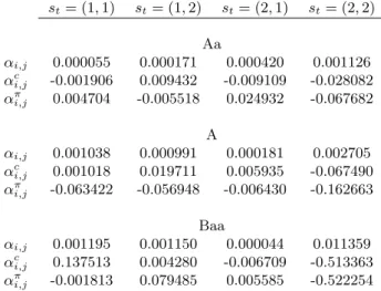
The minimization of the above function is done numerically under the constraint that the one-period conditional default probability is non-negative. The estimated parameters of the conditional default probability are shown in Table 5. It is interesting to notice that for each credit classes, the consumption and inflation parameters in state st= (2, 2) are large negative numbers, indicating that
large negative values for these variables will increase the one period conditional default probability specified as ht= αst+ α
c stct+ α
π stπt.
Figure 9 reproduces the estimated one period conditional default probability computed as 1−
q (t, 1,bα) along with the consumption growth and inflation. It is interesting to note that the
conditional default probability jumps during state st = (2, 2) i.e. the low level high volatility
of consumption growth and high volatility of inflation. These periods are within two out of the three NBER economic recessions found in our sample. Table 6 reports the correlation between consumption and inflation along with their correlations with the estimated default probabilities.
Without any conditioning on the regimes, the estimated probabilities for all credit classes are negatively correlated with the real consumption growth rate with estimated correlations around −0.5 over the 1987-2008 period. However, these signs are changing when conditioning on the regime. For state st = (2, 2), the correlation is around−0.4 for all classes but switches in sign for
credit class. For inflation, without conditioning on the regime, the estimated probabilities are also negatively linked with the probabilities. As for consumption, the correlation is strong and negative in state st= (2, 2). For the other states, the signs change across the different credit classes.
3.6 Recovery rates
The loss given default parameters Li,j (1-the recovery rate) are estimated with an annual time
series of recovery rates from Moody’s (2009) for the years 1987 to 2008. Moody’s rates are defined as the ratio of the defaulted bond’s market price to its face value, as observed 30 days after the default date, for all bonds irrespective of their rating. Because these recovery rates are for all bond ratings, they can be interpreted as the recovery rates of bonds with an average risk.
The limited length of the annual 1987-2008 time series makes it difficult to obtain meaningful estimates for all four possible states. Because of this, we assume a recovery rate varying with the states of consumption only. We obtain an average recovery rate of 0.41 for the state of low volatility of consumption growth (years 1987 to 1989 and 1992 to 2006) prevailing in our 1987-2008 sample period and an average of 0.38 for the high volatility state (years 1990 to 1991 and 2007 to 2008).
3.7 Default spreads in corporate yield spreads
With the parameters of our default spread model obtained from consumption, inflation, risk-free yields, and default data, we examine the theoretical default spreads generated by the model. As mentioned in the introduction, the default spread estimates are computed without using the actual corporate yield spreads to avoid the potential bias associated with missing factors.
Figure 10 plots a two scale graph showing the evolution of the estimated default spread for ten years to maturity Aa, A and Baa zero-coupon bonds in conjunction with the observed yield spread for the case of the constant preference parameter estimates i.e. with bγ = 0.7919 and
b
β ={0.9999, 0.9984, 0.9925, 0.9999}. As shown by the graphs, the estimated default spreads show
some similarities with the observed yields spreads. For example, the sharp increases at the end of 1990 and in 2007-08 are well captured by the model, without the use of yield spread data. The 2001 sharp increase is however not captured by our model. Figure 6 indicates that our observed factors do not show large variations for this 2001 NBER recession. Hence, our model, which specifies
default probabilities that are functions of these state variables, is unable to capture the spread increase for this period.
Table 7 presents statistics concerning these estimated default spreads. This table also reports the statistics across the different states of consumption and inflation. The estimated default spread represents, on average, 8% and 14% and 37% of the 10-year yield spreads for A, Aa and Baa bonds. For Baa bonds, this is higher than numbers found in Elton et al. (2001), who reported a maximum of 25% from an analysis partially using the same data. For Aa and A bonds, the proportions are roughly stable across the different states of the Markov-switching process. For Baa bonds, this proportion varies in the different states. For example, in state st = (1, 2), the high
consumption growth and volatile inflation state, the proportion is 43% while it goes down to 28% in state st = (2, 2), the low consumption and high volatility of inflation state. For this state, the
default spreads showed sharp increases, but not as large as the increases observed for the credit spreads. Further, the volatility of our theoretical default spreads are small when compared with the yield spread volatility for the whole sample and in all subperiods. In general, our estimated default spreads are positively related to the yields spreads with correlations around 50% for all states. Across the different regimes, these correlations are typically positive and strong in state st = (2, 2). For the other states, this correlation is changing in sign across the different ratings.
This indicates that an increase in default spread is not typically linked to an increase in the overall spread.
The correlation of the default spreads with consumption and inflation is negative. When con-ditioning on the possible states, we observe that this link with consumption is not constant across the different regimes and ratings except for state st= (2, 2) which is negative for all ratings. Figure
11 shows the links between our estimated spreads and our observed factors for Baa bonds. Much of the variation is found for state st= (2, 2). For the other states, the positive or negative relations are
weak because the estimated default spreads do not vary much when the factors are varied. Similar pictures are obtained for the Aa and A rating classes.
The part of the default spread associated with the default premium is estimated to be negligible. Hence, using the preference parameters from the fit of the theoretical risk-free yield curves with the observed yield curves, we compute default risk premia that are small, relative to our default spread.
The expression for the one period yield spread shows that the risk aversion parameter impacts on the spreads through the squared volatilities and covariance; it is a second order effect caused by the convexity of our pricing kernel and approximate recovery factor. A possible explanation for the low default premium spread obtained here is thus the low volatility levels of consumption growth and inflation. For reasonable values of the risk aversion parameter, these low volatilities do not easily produce high default premia. In other words, given the estimated volatility levels, a much higher value for the risk-aversion coefficient would be required to generate higher default premia.
We examine here the robustness of our results to the preference parameter estimates. Table 8 presents the credit spreads and proportions computed with the time-varying set of preference parameters estimated in Section 3.4. The results are similar to those from the constant preference parameter presented in Table 7. This can be explained by looking at equations (8) and (9), which show that the theoretical expressions for the default spread is a function of the risk-aversion pa-rameter only, i.e. the time preference papa-rameters in the Apn,st and A
v
n,st functions cancel each other
out. Given that, at the current level of volatilities, the theoretical default spreads are not sensitive to the risk aversion parameter, the constant and time varying parameter estimates for γ produce similar results, even if the two estimates are different on average.
4
Credit default swaps
To get more insights about the capacity of the model developed above to estimate aggregate default proportions, we examine here credit default swaps (CDS hereafter). CDS are insurance contracts written on the notional value of a corporate bond. In case of default, the insured party delivers the bond and gets the notional value from the insurer. To benefit from the insurance protection, the insured pays the CDS premium regularly to the insurer over the life of the contract or until the time of default. Typically, the CDS premium is paid on a quarterly basis with a contract life of 5 years. It is clear that such CDS premia should reflect the possibility of default without any of the tax effects potentially present with bonds. However, as pointed in Jarrow (2010) and Berndt et al (2007), CDS premia are also expected to include the effect of asymmetric information monitoring costs, and a liquidity risk premium due to a quantity impact of trades on the price.
rating classes. It should be noticed that we will focus on CDS premia for zero-coupon bonds, as in our previous analysis. In reality, CDS are written on bonds with coupons. The model developed here is thus used as rough approximation allowing us to see how much of the aggregate CDS premia our default risk model can explain. It should also be mentioned that, as is it the case with bonds, our model for CDS premia only accounts for default. Hence, given that other factors can influence the magnitude of a CDS premium, we expect that the default CDS premia estimated with our model will explain less than 100% of these observed quantities.
4.1 Pricing model
In our zero-coupon corporate bond pricing model, the value of a CDS premium is obtained by solving for the quarterly payment which makes the present value of the future premia (the premium leg) equal to the protection value (the protection leg). The premium leg pays w4 dollars every quarter until maturity if there is no default or until the time of default. The risk of such cash-flows is linked with the possibility of default for the firm. The proper discount factor for these is thus a corporate zero-coupon bond price paying one dollar at maturity, with a loss given default of 100%, since the full payment is lost in case of default. Hence, the present value of the premium leg is written as:
Vpremium(t, n, st) = wst 4 n−1 ∑ i=0 V (t, i, st| Lst = 1) .
The protection leg consists of a single payment at default time. Typically, this payment is equal to the face value of the bond (in exchange of the defaulted bond). In our framework, it is not possible to build a closed form approximation for such a payment. We instead assume that the payment takes the form of a zero-coupon risk-free bond in exchange of the defaulted bond at the time of default. This risk-free zero-coupon bond is the discounted insured face value of the zero-coupon corporate bond. Such an assumption amounts to say that holding a risky bond and the protection leg of the CDS is equivalent to hold a risk-free zero-coupon bond (see Duffie 1999) i.e.
V (t, n, st) + Vprotection(t, n, st) = P (t, n, st)
which leads to
Equating the premium leg with the protection leg and solving for the annual premia w leads to the following formula that is used in the empirical analysis that follows:
wst = 4×
P (t, n, st)− V (t, n, st)
∑n−1
i=0 V (t, i, st| Lst = 1)
. (18)
4.2 Data and results
The CDS data is from Credit Market Analysis and available in Datastream. The CDS data cover the years 2003 to 2008 and gives CDS premia for individual firms with various ratings. The data is aggregated as follows. First, all data points with a veracity score of 4 and higher are discarded6. Second, all maturities different from 5 years are discarded since this is typically the most actively traded maturity. A rating is then assigned to each CDS premium using the firm’s S&P rating at the date of the reported CDS premium. For each quarter of years 2003 to 2008, we aggregate the data by computing the median of the CDS premia for different credit classes. Medians are used because the distribution of the CDS premia at a given time point contains few extreme observations making the mean a doubtful measure of central tendency.
The results of the comparison between our theoretical CDS and observed CDS premia are reported in table 9. As in the previous sections, the theoretical CDS premia are computed with the parameters obtained from the calibration steps. The fixed preference parameter set is used. These estimated default proportions represent, on average, 21%, 35% and 76% of the 5-year CDS premia for A, Aa and Baa ratings. As expected, these default CDS premia do not explain 100% of the observed CDS premia since our model omit the effect of other factors such as the asymmetric information monitoring costs and liquidity (see Jarrow (2010)). In order to make meaningful comparisons, the second panel of this table reports the estimated default spreads and proportions obtained with corporate yield spreads for the same maturity (5 years) and period. These proportions are 6%, 12% and 37% for Aa, A and Baa rated bonds. Thus, as expected, the proportions of default in observed CDS premia are higher than those obtained with bonds. It should be noticed, however, that the estimated default CDS premia in the top panel are roughly equal to the estimated default
6
The “veracity score” is an indicator of the quality of the reported data. A score of 1 is an actual trade; a score of 2 is a ”firm quote” while a score of 3 is a quote. Scores higher than 3 are for data points obtained with some form of interpolation.
spreads in the bottom panel, showing the coherence of the model to estimate default components with different instruments. Again, the average premia are roughly the same across each state, except for the recession state where they increase. This confirms that default can be linked to an undiversifiable macroeconomic default risk factor. For Aa and A ratings, the proportions for both CDS and yield spreads are roughly stable across the different states of the Markov-switching process. For Baa ratings, this proportion varies in the different states. In state st = (1, 2), the
high consumption growth and volatile inflation state, the proportion is 95% while it goes down to 62% in state st = (1, 1), the high consumption growth and low volatility of inflation state. As it
is the case with yield spreads, the volatility of our theoretical default CDS premia are small when compared with the CDS premia volatility.
5
Conclusion
We proposed here an approach for estimating the default spread component of corporate yield spreads. Our model uses observed macroeconomic factors in a reduced form framework and is built on the objective measure. We use a pricing model with discrete regime shifts in consumption growth and inflation. The parameters of consumption, inflation, and conditional default probability variations over time are also functions of the discrete regime shifts. Using consumption, inflation, risk-free yield, and default data, the model is calibrated over the 1987-2008 period.
Our results indicate that our factors are linked to sharp increases in default spreads in two out of three NBER economic recessions. During these recessions, both inflation and consumption growth are negatively linked with default spreads. This result indicate that, in some regimes, the spread level is sensitive to a macroeconomic market-wide undiversifiable risk. Our results also indicate that sharp increases in spreads are not necessarily linked to macroeconomic variables. The sharp increase in 2001 is not captured by our model because this period is found to be in a high consumption growth and low inflation risk regime. This result is consistent with the literature on forecasting models indicating that consumption growth hardly registered negative values in 2001. Our results can explain about half of the yield spread for Baa bond, which can be considered as the average bond in the market. This is in line with the recent study of Giesecke et al (2010), who show that, over the last 150 years, default risk represented about fifty percent of credit spreads.
These authors also document that illiquidity of the bond market is probably the main factor that explains the difference between default spread and credit spread. Our results indicate that this illiquidity effect is perhaps stronger in recession periods. An analysis of credit default swap data obtains default components that are of similar magnitude to those estimated with the bond pricing model. These default components results in higher proportions of default in CDS data. This is consistent with the literature which finds that such instruments are much less influenced by other factors such as liquidity and taxes. Finally, we also find that almost all of the estimated default spread is explained by the default risk while a negligible fraction is due to the default risk premium. This finding is explained by the low volatility of the consumption growth and inflation, which are the main drivers of the default risk premium in this model. Two extensions to this research might be to consider different macro factors, more correlated with economic recessions than consumption and to introduce liquidity risk explicitly in the model.
References
[1] Amato, J.D. and M. Luisi, 2006, Macro Factors in the Term Structure of Credit Spreads, Bank of International Settlements, Working Paper 203.
[2] Ang, A., Bekaert, G. and M. Wei , 2008, The term Structure of Real Rates and Expected Inflation, Journal of Finance 63, 797-849.
[3] Bansal, R. and H. Zhou, 2002, Term Structure of Interest Rates with Regime Shifts, The Journal of Finance 57, 1997-2043.
[4] Berndt, A., R. Jarrow and C. Kang, 2007, Restructuring Risk in Credit Default Swaps: an Empirical Analysis, Stochastic Processes and their Applications 117, 1724 - 1749.
[5] Brown, S. and P. Dybvig, 1986, The Empirical Implications of the Cox, Ingersoll, Ross Theory of the Term Structure of Interest Rates, Journal of Finance 41, 617-30.
[6] Carty, L. and J. Fons, 1993, Measuring Changes in Credit Quality, Journal of Fixed Incomes 4, 27-41.
[7] Carty, L., 1997, Moody’s Rating Migration and Credit Quality Correlation, 1920-1996, Special Comment, Moody’s Investors Service, New York.
[8] Cenesizoglu, T., and E. Badye, 2010, The Effect of Monetary Policy on Credit Spreads, working paper, HEC Montr´eal.
[9] Chen, L., Collin-Dufresne, P., and R. S. Goldstein, 2009, On the Relation Between Credit Spread Puzzles and the Equity Premium Puzzle, Review of Financial Studies 22, 3367-3409. [10] Christensen, J., E. Hansen, and D. Lando, 2004, Confidence Sets for Continuous-Time Rating